UnibucKernel: A kernel based learning method for complex word identification

UnibucKernel: A kernel-based learning method for complex word

identification

Andrei M. Butnaru and Radu Tudor Ionescu

University of Bucharest Department of Computer Science 14 Academiei, Bucharest, Romania [email protected]

[email protected]

Abstract

In this paper, we present a kernel-based learn-ing approach for the 2018 Complex Word Identification (CWI) Shared Task. Our ap-proach is based on combining multiple low-level features, such as character n-grams, with high-level semantic features that are either au-tomatically learned using word embeddings or extracted from a lexical knowledge base, namely WordNet. After feature extraction, we employ a kernel method for the learning phase. The feature matrix is first transformed into a normalized kernel matrix. For the binary clas-sification task (simple versus complex), we employ Support Vector Machines. For the re-gression task, in which we have to predict the complexity level of a word (a word is more complex if it is labeled as complex by more annotators), we employν-Support Vector

Re-gression. We applied our approach only on the three English data sets containing docu-ments from Wikipedia, WikiNews and News domains. Our best result during the com-petition was the third place on the English Wikipedia data set. However, in this paper, we also report better post-competition results.

1 Introduction

A key role in reading comprehension by non-native speakers is played by lexical complexity. To date, researchers in the Natural Language Pro-cessing (NLP) community have developed sev-eral systems to simply texts for non-native speak-ers (Petersen and Ostendorf,2007) as well as na-tive speakers with reading disabilities (Rello et al.,

2013) or low literacy levels (Specia, 2010). The first task that needs to be addressed by text sim-plification methods is to identify which words are likely to be considered complex. The complex word identification (CWI) task raised a lot of at-tention in the NLP community, as it has been ad-dressed as a stand-alone task by some researchers

(Davoodi et al.,2017). More recently, researchers even organized shared tasks on CWI (Paetzold and Specia,2016a;Yimam et al., 2018). The goal of the 2018 CWI Shared Task (Yimam et al.,2018) is to predict which words can be difficult for a non-native speaker, based on annotations collected from a mixture of native and non-native speak-ers. Although the task features a multilingual data set, we participated only in the English monolin-gual track, due to time constraints. In this paper, we describe the approach of our team, UnibucK-ernel, for the English monolingual track of the 2018 CWI Shared Task (Yimam et al.,2018). We present results for both classification (predicting if a word is simple or complex) and regression (pre-dicting the complexity level of a word) tasks. Our approach is based on a standard machine learn-ing pipeline that consists of two phases: (i) fea-ture extraction and (ii) classification/regression. In the first phase, we combine multiple low-level features, such as character n-grams, with high-level semantic features that are either automati-cally learned using word embeddings (Mikolov et al.,2013) or extracted from a lexical knowledge base, namely WordNet (Miller, 1995; Fellbaum,

1998). After feature extraction, we employ a ker-nel method for the learning phase. The feature matrix is first transformed into a normalized ker-nel matrix, using either the inner product between pairs of samples (computed by the linear kernel function) or an exponential transformation of the inner product (computed by the Gaussian kernel function). For the binary classification task, we employ Support Vector Machines (SVM) (Cortes and Vapnik, 1995), while for the regression task, we employ ν-Support Vector Regression (SVR) (Chang and Lin,2002). We applied our approach only on the three English monolingual data sets containing documents from Wikipedia, WikiNews and News domains. Our best result during the

competition was the third place on the English Wikipedia data set. Nonetheless, in this paper, we also report better post-competition results.

The rest of this paper is organized as follows. Related work on complex word identification is presented in Section2. Our method is presented in Section3. Our experiments and results are pre-sented in Section4. Finally, we draw our conclu-sions and discuss future work in Section5.

2 Related Work

Although text simplification methods have been proposed since more than a couple of years ago (Petersen and Ostendorf, 2007), complex word identification has not been studied as a stand-alone task until recently (Shardlow, 2013), with the first shared task on CWI organized in 2016 (Paetzold and Specia, 2016a). With some excep-tions (Davoodi et al., 2017), most of the related works are actually the system description papers of the 2016 CWI Shared Task participants. Among the top10participants, the most popular classifier is Random Forest (Brooke et al.,2016;Mukherjee et al.,2016;Ronzano et al.,2016;Zampieri et al.,

2016), while the most common type of features are lexical and semantic features (Brooke et al.,

2016;Mukherjee et al.,2016;Paetzold and Specia,

2016b;Quijada and Medero,2016;Ronzano et al.,

2016). Some works used Naive Bayes (Mukherjee et al.,2016) or SVM (Zampieri et al.,2016) along with the Random Forest classifier, while others used different classification methods altogether, e.g. Decision Trees (Quijada and Medero,2016), Nearest Centroid (Palakurthi and Mamidi, 2016) or Maximum Entropy (Konkol,2016). Along with the lexical and semantic features, many have used morphological (Mukherjee et al., 2016;Paetzold and Specia,2016b;Palakurthi and Mamidi,2016;

Ronzano et al., 2016) and syntactic (Mukherjee et al.,2016;Quijada and Medero,2016;Ronzano et al.,2016) features.

Paetzold and Specia(2016b) proposed two en-semble methods by applying either hard voting or soft voting on machine learning classifiers trained on morphological, lexical, and seman-tic features. Their systems ranked on the first and the second places in the 2016 CWI Shared Task. Ronzano et al. (2016) employed Random Forests based on lexical, morphological, semantic and syntactic features, ranking on the third place in the 2016 CWI Shared Task. Konkol (2016)

trained Maximum Entropy classifiers on word oc-currence counts in Wikipedia documents, ranking on the fourth place, after Ronzano et al. (2016).

Wr´obel(2016) ranked on fifth place using a sim-ple rule-based approach that considers one feature, namely the number of documents from Simple En-glish Wikipedia in which the target word occurs.

Mukherjee et al. (2016) employed the Random Forest and the Naive Bayes classifiers based on semantic, lexicon-based, morphological and syn-tactic features. Their Naive Bayes system ranked on the sixth place in the 2016 CWI Shared Task. After the 2016 CWI Shared Task, Zampieri et al.

(2017) combined the submitted systems using an ensemble method based on plurality voting. They also proposed an oracle ensemble that provides a theoretical upper bound of the performance. The oracle selects the correct label for a given word if at least one of the participants predicted the cor-rect label. The results reported byZampieri et al.

(2017) indicate that there is a significant perfor-mance gap to be filled by automatic systems.

Compared to the related works, we propose the use of some novel semantic features. One set of features is inspired by the work ofButnaru et al.

(2017) in word sense disambiguation, while an-other set of features is inspired by the spatial pyra-mid approach (Lazebnik et al., 2006), commonly used in computer vision to improve the perfor-mance of the bag-of-visual-words model (Ionescu et al.,2013;Ionescu and Popescu,2015).

3 Method

The method that we employ for identifying com-plex words is based on a series of features ex-tracted from the word itself as well as the context in which the word is used. Upon having the fea-tures extracted, we compute a kernel matrix using one of two standard kernel functions, namely the linear kernel or the Gaussian kernel. We then ap-ply either the SVM classifier to identify if a word is complex or not, or theν-SVR predictor to de-termine the complexity level of a word.

3.1 Feature Extraction

vow-els and constants from the total number of char-acters in the word. Along with these features, we also quantify the number of consecutively repeat-ing characters, e.g. double consonants. For ex-ample, in the word “innovation”, we can find the double consonant “nn”. We also extract n-grams of 1, 2, 3 and 4 characters, based on the intuition that some complex words tend to be formed of a different set of n-grams than simple words. For instance, the complex word “cognizant” is formed of rare 3-grams, e.g. “ogn” or “niz”, compared to its commonly-used synonym “aware”, which con-tains 3-grams that we can easily find in other sim-ple words, e.g. “war” or “are”.

Other features extracted from the target word are the part-of-speech and the number of senses listed in the WordNet knowledge base (Miller,

1995; Fellbaum, 1998), for the respective word. If the complex word is actually composed of mul-tiple words, i.e. it is amulti-word expression, we generate the features for each word in the target and sum the corresponding values to obtain the features for the target multi-word expression.

In the NLP community, word embeddings ( Ben-gio et al., 2003;Karlen et al., 2008) are used in many tasks, and became more popular due to the word2vec(Mikolov et al.,2013) framework. Word embeddings methods have the capacity to build a vectorial representation of words by assigning a low-dimensional real-valued vector to each word, with the property that semantically related words are projected in the same vicinity of the generated space. Word embeddings are in fact a learned rep-resentation of words where each dimension repre-sents a hidden feature of the word (Turian et al.,

2010). We devise additional features for the CWI task with the help of pre-trained word embeddings provided byword2vec(Mikolov et al.,2013). The first set of features based on word embeddings takes into account the word’s context. More pre-cisely, we record the minimum, the maximum and the mean value of the cosine similarity between the target word and each other word from the sen-tence in which the target word occurs. The intu-ition for using this set of features is that a word can be complex if it is semantically different from the other context words, and this difference should be reflected in the embedding space. Having the same goal in mind, namely to identify if the tar-get word is an outlier with respect to the other words in the sentence, we employ a simple

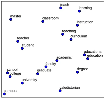
ap-Figure 1: A set of word vectors represented in a 2D space generated by applying PCA on 300-dimensional word embeddings.

proach to compute sense embeddings using the se-mantic relations between WordNet synsets. We note that this approach was previously used for unsupervised word sense disambiguation in ( But-naru et al., 2017). To compute the sense embed-ding for a word sense, we first build a disambigua-tion vocabularyorsense bag. Based on WordNet, we form the sense bag for a given synset by col-lecting the words found in the gloss of the synset (examples included) as well as the words found in the glosses of semantically related synsets. The semantic relations are chosen based on the part-of-speech of the target word, as described in (Butnaru et al.,2017). To derive the sense embedding, we embed the collected words in an embedding space and compute the median of the resulted word vec-tors. For each sense embedding of the target word, we compute the cosine similarity with each and every sense embedding computed for each other word in the sentence, in order to find the mini-mum, the maximum and the mean value.

Using pre-trained word embeddings provided by theGloVeframework (Pennington et al.,2014), we further managed to define a set of useful fea-tures based on the location of the target word in the embedding space. In this last set of features, we first process the word vectors in order to reduce the dimensionality of the vector space from 300 components to only 2 components, by applying Principal Component Analysis (PCA) (Hotelling,

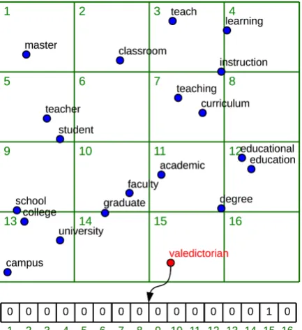
semanti-Figure 2: A grid of4_×4 applied on the 2D embed-ding space. For example, the word “valedictorian” is located in bin number 15. Consequently, the corre-sponding one-hot vector contains a non-zero value at index15.

cally related words, that are projected in the same area of the 2-dimensional (2D) embedding space generated by PCA. In the newly generated space, we apply a grid to divide the space into multiple and equal regions, named bins. This process is inspired by the spatial pyramids (Lazebnik et al.,

2006) used in computer vision to recover spatial information in the bag-of-visual-words (Ionescu et al., 2013; Ionescu and Popescu, 2015). After we determine the bins, we index the bins and en-code the index of the bin that contains the target word as a one-hot vector. Various grid sizes could provide a more specific or a more general location of a word in the generated space. For this reason, we use multiple grid sizes starting from coarse di-visions such as2×2, 4×4, and 8×8, to fine divisions such as16×16and32×32. In Figure2, we show an example with a4_×4grid that divides the space illustrated in Figure1into 16 bins, and the word “valedictorian” is found in bin number 15. The corresponding one-hot vector, containing a single non-zero value at index 15, is also illus-trated in Figure2. The thought process for using this one-hot representation is that complex words tend to reside alone in the semantic space gener-ated by the word embedding framework.

We would like to point out that each and

ev-ery type of features described in this section has a positive influence on the overall accuracy of our framework.

3.2 Kernel Representation

Kernel-based learning algorithms work by embed-ding the data into a Hilbert space and by searching for linear relations in that space, using a learning algorithm. The embedding is performed implic-itly, that is by specifying the inner product be-tween each pair of points rather than by giving their coordinates explicitly. The power of ker-nel methods (Ionescu and Popescu,2016; Shawe-Taylor and Cristianini, 2004) lies in the implicit use of a Reproducing Kernel Hilbert Space in-duced by a positive semi-definite kernel function. Despite the fact that the mathematical meaning of a kernel is the inner product in a Hilbert space, another interpretation of a kernel is the pairwise similarity between samples.

The kernel function offers to the kernel methods the power to naturally handle input data that is not in the form of numerical vectors, such as strings, images, or even video and audio files. The kernel function captures the intuitive notion of similar-ity between objects in a specific domain and can be any function defined on the respective domain that is symmetric and positive definite. In our ap-proach, we experiment with two commonly-used kernel functions, namely the linear kernel and the Radial Basis Function (RBF) kernel. The linear kernel is easily obtained by computing the inner product of two feature vectorsxandz:

k(x, z) =_hx, z_i,

whereh·,·idenotes the inner product. In a similar manner, theRBF kernel(also known as the Gaus-sian kernel) between two feature vectorsx andz can be computed as follows:

k(x, z) =exp

−1− hx, zi

2σ2

.

In the experiments, we replace 1/(2σ2) with a constant valuer, and tune the parameterrinstead ofσ.

step gives to each feature an approximately equal contribution to the similarity between two sam-ples. The normalization of a pairwise kernel ma-trixK containing similarities between samples is obtained by dividing each component to the square root of the product of the two corresponding diag-onal elements:

ˆ Kij =

Kij

p

Kii·Kjj

.

3.3 Classification and Regression

In the case of binary classification problems, kernel-based learning algorithms look for a dis-criminant function, a function that assigns+1 to examples that belong to one class and −1to ex-amples that belong to the other class. This func-tion will be a linear funcfunc-tion in the Hilbert space, which means it will have the form:

f(x) =sign(_hw, x_i+b),

for some weight vectorw and some bias term b. The kernel can be employed whenever the weight vector can be expressed as a linear combination of the training points, Pn

i=1

αixi, implying thatf can

be expressed as follows:

f(x) =sign

n

X

i=1

αik(xi, x) +b

!

,

wherenis the number of training samples andk is a kernel function.

Various kernel methods differ in the way they find the vector w(or equivalently the dual vector α). Support Vector Machines (Cortes and Vap-nik,1995) try to find the vectorwthat defines the hyperplane that maximally separates the images (outcomes of the embedding map) in the Hilbert space of the training examples belonging to the two classes. Mathematically, the SVM classifier chooses the weightswand the bias termbthat sat-isfy the following optimization criterion:

min

w,b

1 n

n

X

i=1

[1₋yi(hw, φ(xi)i+b)]++ν||w||2,

whereyiis the label (+1/−1) of the training

exam-plexi,ν is a regularization parameter and[x]+ =

max{x,0}. We use the SVM classifier for the binary classification of words into simple versus complex classes. On the other hand, we employ

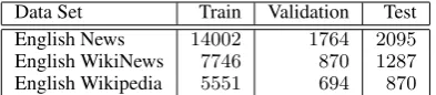
Data Set Train Validation Test English News 14002 1764 2095 English WikiNews 7746 870 1287 English Wikipedia 5551 694 870

Table 1: A summary with the number of samples in each data set of the English monolingual track of the 2018 CWI Shared Task.

ν-Support Vector Regression (ν-SVR) in order to predict the complexity level of a word (a word is more complex if it is labeled as complex by more annotators). Theν-Support Vector Machines (Chang and Lin, 2002) can handle both classifi-cation and regression. The model introduces a new parameterν, that can be used to control the amount of support vectors in the resulting model. The parameterνis introduced directly into the op-timization problem formulation and it is estimated automatically during training.

4 Experiments

4.1 Data Sets

The data sets used in the English monolingual track of the 2018 CWI Shared Task (Yimam et al.,

2018) are described in (Yimam et al.,2017). Each data set covers one of three distinct genres (News, WikiNews and Wikipedia), and the samples are annotated by both native and non-native English speakers. Table1presents the number of samples in the training, the validation (development) and the test sets, for each of the three genres.

4.2 Classification Results

Parameter Tuning.For the classification task, we used the SVM implementation provided by Lib-SVM (Chang and Lin, 2011). The parameters that require tuning are the parameterrof the RBF kernel and the regularization parameterC of the SVM. We tune these parameters using grid search on each of the three validation sets included in the data sets prepared for the English monolin-gual track. For the parameterr, we select values from the set {0.5,1.0,1.5,2.0_}. For the regular-ization parameter C we choose values from the set{10−1,100,101,102_}. Interestingly, we obtain the best results with the same parameter choices on all three validation sets. The optimal parameter choices areC = 101 andr = 1.0. We use these parameters in all our subsequent classification ex-periments.

Data Set Kernel Accuracy F1-score Competition Rank Post-Competition Rank

English News linear 0.8653 0.8547 0.8111∗ 12 6

English News RBF 0.8678 0.8594 0.8178∗ 10 5

English WikiNews linear 0.8205 0.8151 0.7786∗ _{10 5}

English WikiNews RBF 0.8252 0.8201 0.8127∗ 5 4

English Wikipedia linear 0.7874 0.7873 0.7804∗ 6 4 English Wikipedia RBF 0.7920∗ 0.7919∗ 0.7919∗ 3 3

Table 2: Classification results on the three data sets of the English monolingual track of the 2018 CWI Shared Task. The methods are evaluated in terms of the classification accuracy and theF1-score. The results marked with

an asterisk are obtained during the competition. The other results are obtained after the competition.

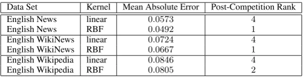
Data Set Kernel Mean Absolute Error Post-Competition Rank

English News linear 0.0573 4

English News RBF 0.0492 1

English WikiNews linear 0.0724 4

English WikiNews RBF 0.0667 1

English Wikipedia linear 0.0846 4

English Wikipedia RBF 0.0805 2

Table 3: Regression results on the three data sets of the English monolingual track of the 2018 CWI Shared Task. The methods are evaluated in terms of the mean absolute error (MAE). The reported results are obtained after the competition.

the three data sets included in the English mono-lingual track are presented in Table2. We would like to note that, before the competition ended, we observed a bug in the code that was used in most of our submissions. In the feature extraction stage, the code produced NaN (not a number) values for some features. In order to make the submissions in time, we had to eliminate the samples containing NaN values in the feature vector. Consequently, most of our results during the competition were lower than expected. However, we managed to fix this bug and recompute the features in time to re-submit new results, but only for the RBF kernel on the English Wikipedia data set. The rest of the results presented in Table2are produced after the bug fixing and after the submission deadline. Nev-ertheless, for a fair comparison with the other sys-tems, we include ourF1-scores and rankings

dur-ing the competition as well as the post-competition F1-scores and rankings.

The results reported in Table2indicate that the RBF kernel is more suitable for the CWI task than the linear kernel. Our bestF1-score on the English

News data set is 0.8594, which is nearly 1.4% lower than the top scoring system, which attained 0.8736 during the competition. On the English WikiNews data set, our bestF1-score (0.8201) is

once again about 2% lower than the top scoring system, which obtained 0.8400 during the com-petition. On the English Wikipedia data set, our best F1-score is 0.7919. With this score, we

ranked as the third team on the English Wikipedia data set. Two systems performed better on En-glish Wikipedia, one that reached the topF1-score

of 0.8115 and one that reached the second-best scored of0.7965. Overall, our system performed quite well, but it can surely benefit from the addi-tion of more features.

4.3 Regression Results

Although we did not submit results for the regres-sion task, we present post-competition regresregres-sion results in this section.

Parameter Tuning. For the regression task, the parameters that require tuning are the parameterr of the RBF kernel and theν-SVR parametersC andν. As in the classification task, we tune these parameters using grid search on the validation sets provided with the three data sets included in the English monolingual track. For the parameterr, we select values from the set{0.5,1.0,1.5,2.0}. For the regularization parameterCwe choose val-ues from the set{10−1_,100_,101_,102_{}. The}

Results. The regression results on the three data sets included in the English monolingual track are presented in Table 3. The systems are evaluated in terms of the mean absolute error (MAE). As in the classification task, we can observe that the RBF kernel provides generally better results than the linear kernel. On two data sets, English News and English WikiNews, we obtain better MAE val-ues than all the systems that participated in the competition. Indeed, the best MAE on English News reported during the competition is 0.0510, and we obtain a smaller MAE (0.0492) using the RBF kernel. Similarly, with a MAE of 0.0667 for the RBF kernel, we surpass the top system on English WikiNews, which attained a MAE of 0.0674during the competition. On the third data set, English Wikipedia, we attain the second-best score (0.0805), after the top system, that obtained a MAE of 0.0739during the competition. Com-pared to the classification task, we report better post-competition rankings in the regression task. This could be explained by two factors. First of all, the number of participants in the regression task was considerably lower. Second of all, we be-lieve thatν-SVR is a very good regressor which is not commonly used, surpassing alternative regres-sion methods in other tasks as well, e.g. image difficulty prediction (Ionescu et al.,2016).

5 Conclusion

In this paper, we described the system developed by our team, UnibucKernel, for the 2018 CWI Shared Task. The system is based on extract-ing lexical, syntatic and semantic features and on training a kernel method for the prediction (clas-sification and regression) tasks. We participated only in the English monolingual track. Our best result during the competition was the third place on the English Wikipedia data set. In this paper, we also reported better post-competition results.

In this work, we treated each English data set independently, due to the memory constraints of our machine. Nevertheless, we believe that join-ing the trainjoin-ing sets provided in the English News, the English WikiNews and the English Wikipedia data sets into a single and larger training set can provide better performance, as the model’s gener-alization capacity could improve by learning from an extended set of samples. We leave this idea for future work. Another direction that could be explored in future work is the addition of more

features, as our current feature set is definitely far from being exhaustive.

References

Yoshua Bengio, R´ejean Ducharme, Pascal Vincent, and Christian Jauvin. 2003. A neural probabilistic lan-guage model. Journal of Machine Learning Re-search, 3(Feb):1137–1155.

Julian Brooke, Alexandra Uitdenbogerd, and Timothy Baldwin. 2016. Melbourne at SemEval 2016 Task 11: Classifying Type-level Word Complexity using Random Forests with Corpus and Word List Fea-tures. In Proceedings of SemEval, pages 975–981, San Diego, California. Association for Computa-tional Linguistics.

Andrei M. Butnaru, Radu Tudor Ionescu, and Flo-rentina Hristea. 2017. ShotgunWSD: An unsuper-vised algorithm for global word sense disambigua-tion inspired by DNA sequencing. InProceedings of EACL, pages 916–926.

Chih-Chung Chang and Chih-Jen Lin. 2002. Train-ing ν-Support Vector Regression: Theory and

Al-gorithms. Neural Computation, 14:1959–1977.

Chih-Chung Chang and Chih-Jen Lin. 2011. LibSVM: A Library for Support Vector Machines. ACM Transactions on Intelligent Systems and Technol-ogy, 2:27:1–27:27. Software available athttp://

www.csie.ntu.edu.tw/˜cjlin/libsvm.

Corinna Cortes and Vladimir Vapnik. 1995. Support-Vector Networks. Machine Learning, 20(3):273– 297.

Elnaz Davoodi, Leila Kosseim, and Matthew Mon-grain. 2017. A Context-Aware Approach for the Identification of Complex Words in Natural Lan-guage Texts. InProceedings of ICSC, pages 97–100.

Christiane Fellbaum, editor. 1998. WordNet: An Elec-tronic Lexical Database. MIT Press.

Harold Hotelling. 1933. Analysis of a complex of sta-tistical variables into principal components. Journal of Educational Psychology, 24(6):417.

Radu Tudor Ionescu, Bogdan Alexe, Marius Leordeanu, Marius Popescu, Dim Papadopou-los, and Vittorio Ferrari. 2016. How hard can it be? Estimating the difficulty of visual search in an image. InProceedings of CVPR, pages 2157–2166.

Radu Tudor Ionescu and Marius Popescu. 2015. PQ kernel: a rank correlation kernel for visual word his-tograms. Pattern Recognition Letters, 55:51–57.

Radu Tudor Ionescu and Marius Popescu. 2016.

Radu Tudor Ionescu, Marius Popescu, and Cristian Grozea. 2013. Local Learning to Improve Bag of Visual Words Model for Facial Expression Recog-nition. Workshop on Challenges in Representation Learning, ICML.

Michael Karlen, Jason Weston, Ayse Erkan, and Ronan Collobert. 2008. Large scale manifold transduction. InProceedings of ICML, pages 448–455. ACM.

Michal Konkol. 2016. UWB at SemEval-2016 Task 11: Exploring Features for Complex Word Identi-fication. In Proceedings of SemEval, pages 1038– 1041, San Diego, California. Association for Com-putational Linguistics.

Svetlana Lazebnik, Cordelia Schmid, and Jean Ponce. 2006. Beyond Bags of Features: Spatial Pyra-mid Matching for Recognizing Natural Scene Cat-egories.Proceedings of CVPR, 2:2169–2178.

Tomas Mikolov, Ilya Sutskever, Kai Chen, Gregory S. Corrado, and Jeffrey Dean. 2013. Distributed Rep-resentations of Words and Phrases and their Compo-sitionality.Proceedings of NIPS, pages 3111–3119.

George A. Miller. 1995. WordNet: A Lexical Database for English. Communications of the ACM, 38(11):39–41.

Niloy Mukherjee, Braja Gopal Patra, Dipankar Das, and Sivaji Bandyopadhyay. 2016. JU NLP at SemEval-2016 Task 11: Identifying Complex Words in a Sentence. In Proceedings of SemEval, pages 986–990, San Diego, California. Association for Computational Linguistics.

Gustavo Paetzold and Lucia Specia. 2016a. SemEval 2016 Task 11: Complex Word Identification. In Pro-ceedings of SemEval, pages 560–569, San Diego, California. Association for Computational Linguis-tics.

Gustavo Paetzold and Lucia Specia. 2016b. SV000gg at SemEval-2016 Task 11: Heavy Gauge Complex Word Identification with System Voting. In Pro-ceedings of SemEval, pages 969–974, San Diego, California. Association for Computational Linguis-tics.

Ashish Palakurthi and Radhika Mamidi. 2016. IIIT at SemEval-2016 Task 11: Complex Word Identifica-tion using Nearest Centroid ClassificaIdentifica-tion. In Pro-ceedings of SemEval, pages 1017–1021, San Diego, California. Association for Computational Linguis-tics.

Jeffrey Pennington, Richard Socher, and Christo-pher D. Manning. 2014. GloVe: Global Vectors for Word Representation. In Proceedings of EMNLP, pages 1532–1543.

Sarah E. Petersen and Mari Ostendorf. 2007. Text Sim-plification for Language Learners: A Corpus Analy-sis. InProceedings of SLaTE.

Maury Quijada and Julie Medero. 2016. HMC at SemEval-2016 Task 11: Identifying Complex Words Using Depth-limited Decision Trees. In Proceed-ings of SemEval, pages 1034–1037, San Diego, Cal-ifornia. Association for Computational Linguistics.

Luz Rello, Ricardo Baeza-Yates, Stefan Bott, and Ho-racio Saggion. 2013. Simplify or Help?: Text Sim-plification Strategies for People with Dyslexia. In

Proceedings of W4A, pages 15:1–15:10.

Francesco Ronzano, Ahmed Abura’ed, Luis Es-pinosa Anke, and Horacio Saggion. 2016. TALN at SemEval-2016 Task 11: Modelling Complex Words by Contextual, Lexical and Semantic Features. In

Proceedings of SemEval, pages 1011–1016, San Diego, California. Association for Computational Linguistics.

Matthew Shardlow. 2013. A Comparison of Tech-niques to Automatically Identify Complex Words. InProceedings of the ACL Student Research Work-shop, pages 103–109.

John Shawe-Taylor and Nello Cristianini. 2004. Ker-nel Methods for Pattern Analysis. Cambridge Uni-versity Press.

Lucia Specia. 2010. Translating from complex to simplified sentences. InProceedings of PROPOR, pages 30–39.

Joseph Turian, Lev Ratinov, and Yoshua Bengio. 2010. Word representations: a simple and general method for semi-supervised learning. In Proceedings of ACL, pages 384–394. Association for Computa-tional Linguistics.

Krzysztof Wr´obel. 2016. PLUJAGH at SemEval-2016 Task 11: Simple System for Complex Word Iden-tification. In Proceedings of SemEval, pages 953– 957, San Diego, California. Association for Compu-tational Linguistics.

Seid Muhie Yimam, Chris Biemann, Shervin Mal-masi, Gustavo Paetzold, Lucia Specia, Sanja ˇStajner, Ana¨ıs Tack, and Marcos Zampieri. 2018. A Report on the Complex Word Identification Shared Task 2018. In Proceedings of BEA-13, New Orleans, United States. Association for Computational Lin-guistics.

Seid Muhie Yimam, Sanja ˇStajner, Martin Riedl, and Chris Biemann. 2017. CWIG3G2 - Complex Word Identification Task across Three Text Genres and Two User Groups. InProceedings of IJCNLP (Vol-ume 2: Short Papers), pages 401–407, Taipei, Tai-wan.