Phase coherence theory for data-mining and analysis:
Application studies in spectroscopy
G. Doyle
1, N.D. McMillan
1, F. Murtagh
3, M. O’Neill
1, S. Riedel
1, T.S. Perova
2, S. Unnikrishnan
2,
and R.A. Moore
21
Institute of Technology Carlow, Carlow, Ireland
2Dept. of Electronic and Electrical Engineering, Trinity College, Dublin 2, Ireland,
3Dept. of Computer Science, Royal Holloway, University of London, Egham, Surrey, England
ABSTRACT
1. INTRODUCTION
The science of tensiography can simply be stated as the extraction of physical, chemical and product information from the instrumental tensiotrace using computer science methods. The tensiograph produces graphical data display, which is obtained from detecting the light injected inside a growing pendant drop by a source fiber and coupled to a collector fiber via various reflections inside the drop. Phase Coherence Theory (PCT) was developed by McMillan et al. [1] for tensiographic data mining and analysis. The data mining, data visualisation, statistical and data analysis package, TraceMiner V2.6, developed by Doyle and McMillan integrates the phase coherent data scatter algorithm and additional PCT techniques with many standard parametric and non-parametric statistical tests [2]. This software was developed as a generic, extensible, portable and easy to use data mining and analysis toolkit, supporting visualisation and statistics using object oriented software development techniques in the C++ programming language.
The advantage of the PCT data-scatter approach is that it allows the user to experimentally investigate a data mining and analysis problem and identify the most appropriate TraceMiner toolkit utility for the problem at hand. This point is borne out by the fact that, of a large number of toolkit utilities available to the researcher, only a small number will typically be relevant to a specific data-mining problem. The toolkit is designed to produce measurements from statistics, rather than merely posing the statistical question as to whether or not two data sets are the same.
The software toolkit has been used for tensiographic data mining and analysis. The developers’ objective, however, to create a generic, cross-platform toolkit has now been realised with the application of the toolkit to Raman spectroscopy [3] for composition and defect analysis in semiconductor structures. The sensitive nature of phase coherent data scatter and the other TraceMiner toolkit techniques provided the potential for small spectral changes observed to be identified and quantified successfully for Raman spectroscopy.
The work described in this paper involved investigating the practicality of the data-scattering method for the analysis of Raman spectra and establishing the dependence of changes obtained in all the spectral function characteristics on the measurands of data-scatter. The experimental and modeling work was done in Perova and Unnkrishnan in Trinity and O’Neill in Carl Stuart using TraceMiner. The results provide support for the general utility of the data mining toolkit and the validation was done by O’Neill, McMillan and Doyle.
Raman spectroscopy is a widely used composition and defect analysis technique in semiconductor structures. The need for a sensitive analysis algorithm is apparent as the difference in Raman spectral characteristics such as the peak position (ωmax), the peak intensity (Imax) and the full width at half maximum (FWHM), which can be used to gain
information on different properties of studied materials and in particular, at the stage of their fabrication, can be minute. For example, the shift of the phonon lines in stressed semiconductors from the unstressed value can be as small as 0.05 cm-1 (at maximum spectral resolution of ~1 cm-1). It is noted that this shift is directly related to the stress value, so it is important to estimate the shift with higher accuracy. To date, the fitting of the phonon bands with Lorentzian or Gaussian functions is used in order to determine the peak position with accuracy < 0.1 cm-1. Nevertheless, for certain types of semiconductors (particularly nanostructured ones) the shape of the phonon line is also distorted due to the confinement effect and stress, making the proper fitting of these lines quite difficult.
As the need for new methods of analysis to quantify small changes observed in the registered spectral function for a semiconductor surface is clear, the PCT data mining measurands of scatter radius, scatter coherence and scatter closeness are innovatively applied in this investigation to establish the dependence of spectral changes obtained in all Raman spectral characteristics previously mentioned.
2. THEORY
2.1 The data mining software
The algorithm customised to meet the specific need to produce scatter of data points that gives visual representations of instrumental performance has been termed Phase Coherent Data-Scatter. The term signifies the phase relationships in data-scatter between the ordinate and abscissa of the two data sets that are being studied. The phase coherent algorithm offers a set of new measurements such as scatter coherence, scatter closeness, and scatter radius values. According to phase coherence theory [1], the most significant measurement of data scatter is ‘coherence’ which gives a numerical measure of the individual error components for the two principal coordinates.
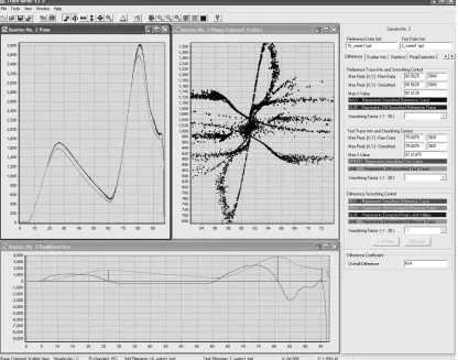
[image:3.612.90.506.313.640.2]Based on this theory, we have developed [2] software for data mining called TraceMiner. The software allows the user to obtain values of coherence scatter for two different spectra (reference and test traces) with respect to their centroid. The centroid is found to be a stable point with respect to spectral variations. But this technique has a drawback that there is a possibility of two different spectra being projected to the same centroid. Hence, it is impossible to distinguish between traces using only the centroid. An exchange operation is employed as a solution to this problem [2]. Phase coherence theory also explains scatter closeness, which gives the Euclidean distance between the two centroids of the unexchanged data in the test and reference traces. This parameter provides a single simple measure of scatter-points. The new coherence theory gives birth to a novel interesting phenomenon, which arises from combinations of digital and propagation errors uprising from the algorithm used, called micro-scatter [2]. This phenomenon can be explained as the pattern observed with zooming magnification of what appeared to be a single centroid. Scatter radii, which gives a quantification of the scatter, is also given importance in the new coherence theory.
The data mining issues considered in the following sections are the stages of data mining and how the TraceMiner software algorithms address them.
2.2 Data Mining Issues
This section presents a detailed examination of the algorithms provided by the TraceMiner toolkit. These algorithms are expounded in a manner that is not specific to the Raman spectroscopy application, allowing us to illustrate the generic utility of the techniques, framed in the context of the major identifiable stages of the data mining and analysis process.
2.2.1 Data ingest (data presentation to the software)
The TraceMiner software is designed using an extensible object oriented design to handle two-dimensional data sets. This is ideal for the problems that have so far been addressed using the software toolkit, namely tensiography where a trace is gathered as a two-dimensional data set (voltage over time), and UV-visible spectroscopy where the data sets gathered are also two-dimensional (absorbance over wavelength). The software tests pairs of data sets where one set is termed the reference set (control set) and the other set is termed the test set and is compared against the reference. All PCT and statistical measures are taken in this context.
Any data set gatherer needs to be cognisant of the fact that the current constitution of data sets for the software means that it can handle all two dimensional data sets that are presented as a white space separated text file. The software will automatically calculate a significant number of statistical measures for the data sets.
2.2.2 Data Cleansing/Smoothing
Data imported into the software toolkit can be smoothed using a moving average with window length from 1 (no smoothing) to 30. The maximum scaling factor is arbitrary and can be changed. However, the developers felt that a larger smoothing factor than this would serve only to obfuscate the original data set to an unrealistic point.
The researcher can choose to smooth the reference and test data sets using the same or different factors. The software will inform the user if the smoothing factor is different when they attempt further processing on the data sets as this may affect the validity of results. Typically both data sets are smoothed to the same degree. The difference curve for two data sets can also be smoothed.
It should be noted that data sets in tensiography typically contain of the order of three thousand data points. The smoothing algorithm helps to enhance important features of a data set by smoothing peaks and filtering inaccurate outliers in the data. The smoothing factor chosen will depend on the application under analysis.
2.2.3 Feature Identification and Extraction
Data sets that have been imported into the software are processed using algorithms to identify the important features of the data sets and the differences between the data sets. The software toolkit provides the researcher with a number of data mining algorithms that allow them to more easily identify and extract the important features of the data sets under investigation. The algorithms are as follows.
1 Phase Coherent Data Scatter.
PCD-S offers tools for feature extraction. The scatter diagram produced by the application of the algorithm when data points are projected back to a single centroid provides the researcher with a visualisation of the difference between two data sets that scatters the differences away from a centre point. This provides a focus on the feature differences that is directly navigable back to the individual data set points and thus potentially important features such as peaks in the original data sets 1.
Un-exchanged Data Scatter.
Exchanged Data Scatter.
Data sets that are not the same may produce identical centroids, leading to the inclusion of an exchange operation that guarantees that differing features in the data sets will be identified on the data scatter diagram.
Scatter Information
The software affords information regarding the data scatter such as the centroid positions for each data set, the scatter closeness, scatter radii and the scatter coherence.
2 Difference Tensiography.
This algorithm performs a data point by data point subtraction of two data sets, reference from test, on the ordinate and thus highlights feature differences of the test data from the reference set and in particular the larger feature differences are identified. If the data sets are of different lengths, the software will pad the shorter trace with zeros4.
The identification and quantification of the point-by-point feature differences in the data sets allows data miners to be particularly focused on feature variations in the data sets and, possibly more importantly, where the maximum differences between the data sets occur, allowing focussed investigation on the divergences.
3 Peak Match and Subtraction (MS) Values.
MS values present a utility that identifies the major peaks in the reference and test data sets and compares them on the basis of how well they match (M values) 6 or how different they are (S values) 7 in terms of the ordinate and abscissa
• Match Values
Normalised M values are calculated by finding each peak in the test data set and comparing it to the equivalent peak, if any, in the reference data set. An M value of one means that a peak in the test set is identical to the equivalent peak in the reference data set. The closer the M value to zero, the less of a match the peaks are.
• Subtraction Values
S Values are complimentary to the M values and highlight how different corresponding peaks in the test and reference data sets are. Adding the normalised MS values together will always produce a value of one. It is possible to adjust the sensitivity of the S values.
4 Statistical Measures
The toolkit provides a range of relevant parametric and non-parametric statistical measures based on Johnson and Bhattacharyya 5 including the following:
a. Basic Statistics
i. Difference Mean
ii. Standard Deviation of Difference iii. Standard Error of Difference Mean
iv. Confidence Interval for the Mean Difference
b. Normal Distribution Checks
i. Fingerprint Test Using Normal Distribution ii. Normal Distribution Test
c. Parametric Statistics
i. Correlation Coefficient ii. Regression Line (Slope) iii. Regression Line (Intercept) iv. Residual Sum of Squares d. Non Parametric Statistics
i. Wilcoxon Rank Sum Test ii. Wilcoxon Signed Rank Test
2.2.4 Pattern Extraction and Discovery
The previous section details the feature identification and extraction algorithms in TraceMiner. At this point the major data mining issue is results analysis and the identification of difference or similarities patterns or measurements that occur in the data sets. The advantage of this approach is generally accepted at this stage to be the fact that visualisations of data differences are given together with measurements on the features and structure of the patterns themselves. The best way of explaining this is to see these patterns as an analogue of x-ray diffraction patterns in that the symmetry and structure of a pattern can be traced back to actual difference and structure in the data sets under test. The most obvious example of this structure is the testing of instrument performance such as a UV-visible spectrophotometer that gives scatter in the vertical direction if the y-errors are present (photometric in UV-visible) and scatter in the horizontal if there are x-errors (wavelength errors in the UV-visible) and loops if both are present. Again with respect to instrument performance, a specific type of noise will give one pattern while another type produces another and thermal and shot noise can thus be differentiated visually. Much more complex patterns are observed than this example used to illustrate the visualisation issues here, but it can be simply stated that there is usually little problem in identifying a pattern with a specific problem.
It is clearly significant that patterns represent local phenomenon within a data set and can thus be traced back to the original data that caused the pattern and investigated further8. Two of the more powerful and readily used methods for pattern recognition are the Hough9 and Radon10 transforms. The data-scatter technique produces recognizable scatter patterns based on the temporal data sets. It is important to qualitatively differentiate the various data groups associated with a feature in a pattern. The Hough or other technique will be used to partition the scatter data points (e.g. to differentiate a line from a curve). The subsequent quantification of this partitioned data can potentially have useful applications.
2.2.5 Visualisation of Data and Results
The toolkit provides extensive visualisation capabilities for both the data sets and the results of the algorithms. These include visualisation of and supplementary information for:
• Untreated imported data sets
• Smoothed data sets
• Difference results (unsmoothed and smoothed)
• MS values
• PCD-S values (unexchanged and exchanged)
Each of the visualisation tools for data sets and results has a zooming feature to aid with identification and assessment of important and unimportant features. On occasion differencing of the data sets using visualisation may be sufficient.
2.2.6 Evaluation of Results
The evaluation of the results provided by the toolkit tends to be specific to the application under study. For example, large parts of the evaluation of results for tensiography and UV-visible spectroscopy have been extensively researched11. Investigation of the significance of results for Raman spectroscopy is ongoing and the results thus far are encouraging.
3. APPLICATION TO RAMAN SPECTROSCOPY
The work below is also presented elsewhere in these proceedings, but Perova et al3 has an experimental emphasis and deals with material science issues where here we restrict the discussion to computer science issues as far as possible.
As previously stated, in the investigation a model oscillator with spectral characteristics close to that of longitudinal optical (LO) phonon mode of bare Si at 520 cm-1 was chosen for the purpose of phase coherent data-scatter analysis. Raman spectra can in general be fitted best by a Lorentzian function
whereω0 is the peak frequency, I0 is the intensity at ω0 and2w is the FWHM. A family of Lorentzian spectral functions
have been modelled using variation in peak position (Raman shift), peak intensity and FWHM. The analysis of these three sets of model spectra was carried out using TraceMiner to extract the parameters of data scattering analysis. In this way, the dependence of each of the data scatter parameters on changes observed in Raman spectral characteristics such as the following was established:
Raman shift, ω RS = ω Test - ω Ref (2)
Raman intensity difference,IRID =ITest - IRef (3) Raman FWHM difference, FWRFD = FWTest - FWRef. (4)
In this study the scatter closeness and scatter radii parameters of phase coherence theory were used.
3.1 Frequency Monitoring
The analysis was carried out by modelling a set of Lorentzian spectral functions by varying the peak frequency from 520 cm-1 to 530 cm-1 and keeping the peak intensity constant at 10000 A.U. and FWHM at 4 cm-1. A step of 0.1 cm-1 from 520 cm-1 to 521 cm-1 and a step of 1 cm-1 from 521 cm-1 to 530 cm-1 were used (Fig. 2).
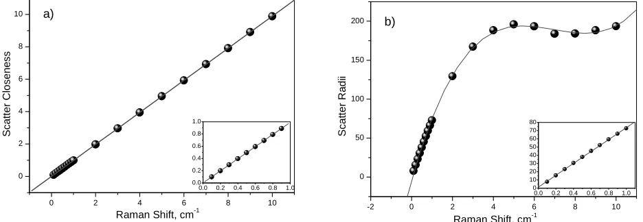
For the above set of model spectra, the values of data-scatter parameters such as scatter radii and scatter closeness were calculated using phase coherence theory by using the model curve with peak frequency at 520 cm-1 as a reference. Fig. 3 shows the dependencies of data-scatter parameters on Raman shift (νRS).
[image:7.612.51.272.260.414.2]
Figure 3 Dependence of scatter closeness (a) and scatter radii (b) on Raman Shift (peak frequency varied from 520 to 530 cm-1). Inset shows the corresponding plots for frequencies ranging from 520 to 521 cm-1 with a step of 0.1 cm-1 respectively.
515 520 525 530 535
0 2000 4000 6000 8000 10000 In te n s it y ( A .U .)
[image:7.612.65.533.461.623.2]Wavenumbers (cm-1)
Figure 2 Set of the Lorentzian spectral
functions with peak position ranging from 520 cm-1 up to 530 cm-1.
0 2 4 6 8 10
0 2 4 6 8 10 a) Sc a tter C los ene s s
Raman Shift, cm-1
0.0 0.2 0.4 0.6 0.8 1.0 0.0 0.2 0.4 0.6 0.8 1.0
-2 0 2 4 6 8 10
0 50 100 150 200 b) Sc at ter R a di i
Raman Shift, cm-1
Scatter closeness gives perfect linear dependence (Fig. 3a) on Raman Shift in the whole frequency range from 520 cm-1 to 530 cm-1 for different step values, which is given by the equation.
Y = 0.989 X (5)
In the case of scatter radii (Fig. 3b), a linear dependence on Raman shift has been observed for frequency values ranging from 520 cm-1 to 521 cm-1 with a step of 0.1 cm-1. When the shift is increased to 1 cm-1, the data points of scatter radii for frequencies ranging from 521 to 530 cm-1 can be best fitted by a polynomial function.
Inspection of Fig. 3a and 3b from a data mining perspective provides some useful information. It can be seen from Fig. 3a that the scatter closeness provides a large dynamic range with good coverage of the entire range of measurements. Scatter radii provide a much smaller dynamic range although the calibration sensitivity is greater than that of scatter closeness (greater slope means greater sensitivity). Examination of the detection limit provided by each measure demonstrates that the scatter closeness detection limit is more sensitive. On balance scatter closeness provides a superior tool for analysing frequency shift as demonstrated here.
3.2 Intensity Monitoring
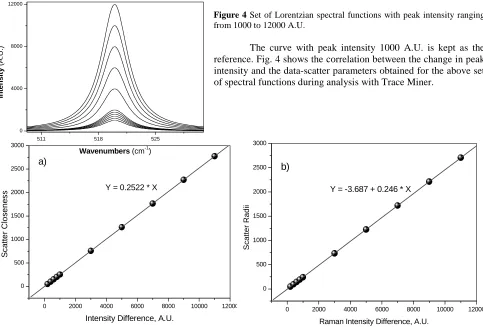
[image:8.612.54.537.296.623.2]A group of Lorentzian spectral functions was modelled by varying the peak intensity from 1000 to 12000 (A.U.) initially with a step of 200 from 1000 to 2000 and then with a step of 2000 from 2000 to 12000 A.U. (Fig. 4). Peak frequency is kept constant at 520 cm-1 and FWHM at 4 cm-1.
Figure 4 Set of Lorentzian spectral functions with peak intensity ranging
from 1000 to 12000 A.U.
The curve with peak intensity 1000 A.U. is kept as the reference. Fig. 4 shows the correlation between the change in peak intensity and the data-scatter parameters obtained for the above set of spectral functions during analysis with Trace Miner.
Figure 5 Dependence of scatter closeness (a) and scatter radii (b) on Raman Intensity Difference (peak intensity varied from 1000 to
12000 A.U)
511 518 525
0 4000 8000 12000 Int e ns it y ( A .U .)
Wavenumbers (cm-1)
0 2000 4000 6000 8000 10000 12000 0 500 1000 1500 2000 2500 3000 a) S c atte r C lo s e nes s
Intensity Difference, A.U. Y = 0.2522 * X
0 2000 4000 6000 8000 10000 12000 0 500 1000 1500 2000 2500 3000 b) S c atte r Ra di i
Raman Intensity Difference, A.U.
Both the data-scatter parameters viz. scatter closeness (Fig. 5a) and scatter radii (Fig. 5b) give linear dependence on Raman intensity difference, which proves to be quite useful in further studies of nanostructures using Raman spectroscopy.
Inspection of Fig. 5a and 5b from a data mining perspective again provides useful information. For example, it can be seen that scatter closeness provides the best measure for peak intensity shifts by providing the better calibration sensitivity. The intercept on the scatter radii plot means that scatter closeness will provide a better detection limit. As well as providing the previously mentioned linear dependence both measures also provide a large dynamic measurement range. However again the scatter closeness provides the more useful measure because of the better calibration sensitivity.
3.3 FWHM Monitoring
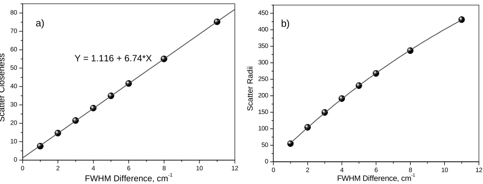
[image:9.612.60.548.446.632.2]By varying the FWHM values from 4 to 15 cm-1 with different steps of 1 cm-1, 2 cm-1 and finally 3 cm-1, a set of Lorentzian spectral functions was created (Fig. 6). The peak position and peak intensity are kept constant at 520 cm-1 at 10000 A.U. respectively.
Figure 6 Lorentzian Spectral Function with FWHM varied from
4 cm-1 to 15 cm-1
The dependence of data-scatter parameters on changes in FWHM of Raman spectra is shown in Fig. 7
Figure 7 Dependence of scatter closeness (a) and scatter radii (b) on Raman FWHM Difference (varied from 4 to 15 cm-1)
490 500 510 520 530 540 550
0 2000 4000 6000 8000
10000 FWHM varied from 4 to 15cm
-1 In te n s ity (A .U .)
Wavenumbers (cm-1)
0 2 4 6 8 10 12
0 50 100 150 200 250 300 350 400 450 b) S c at te r R adi i
FWHM Difference, cm-1
0 2 4 6 8 10 12
0 10 20 30 40 50 60 70 80 a) S c att e r C losen ess
Scatter closeness (Fig. 7a) shows perfect linear dependence, which is in line with linewidth variation, while scatter radii (Fig. 7b) values fit exactly into the sigmoid-Boltzmann function given by the following expression.
y = 884.898 + (-7182.081-884.898)/(1 + exp ((x+32.39)/15.403)) (6)
Note that equation 6 is obtained by curve fitting the scatter radii data points using Origin scientific graphing and analysis software.
However, as can be seen from Fig. 7b, the deviation of scatter radii from non-linearity is practically negligible up to FWHM difference of ~6 cm-1.
Clearly, from a data mining standpoint scatter closeness again provides the more useful measure as it shows a linear dependence, a sensitive detection limit, a large dynamic range and good calibration sensitivity.
3.4 Real Instrumental Data
[image:10.612.57.325.266.422.2]Similar data scatter analysis was performed on experimental Raman spectra of bare Si wafer as part of this work. The experimental curve with peak frequency at 520 cm-1 is taken as a reference. By shifting the reference curve from its initial position with a step of 0.2 cm-1 and 1 cm-1 in the regions of 520-521 cm-1 and 521-530 cm-1 respectively, a set of experimental Raman spectra similar to that shown in Fig. 8 was created.
Figure 8 Experimental Raman spectra of bare
Silicon at 520 cm-1 and the test curves shifted from the experimental curve with a step of 0.2 cm-1 and 1 cm-1 respectively.
As a result of the analysis of these test traces with the reference trace using phase coherence theory, the dependence of scatter closeness on Raman shift was obtained. As shown in Fig. 9, the scatter closeness obtained from the above set of data exhibits perfect linear dependence on Raman shift (ωRS from 0.1 up to 6 cm-1), which is very close
to that obtained for model data shown in Fig. 3a.
On comparison with equation (5), the dependence of scatter closeness obtained for both model and experimental Raman data are approximately coinciding.
Figure 9 Dependence of scatter closeness on experimental
Raman shift (in the range 520 cm-1 to 527 cm-1)
0 1 2 3 4 5 6
0 1 2 3 4 5 6
Sc
atter
Clos
enes
s
R a m a n S h ift , c m- 1
Y = 0 .0 0 1 + 0 . 9 9 9 * X
510 520 530
0 2000 4000 6000
Int
e
ns
ity
(
A
.U
.)
[image:10.612.59.319.495.644.2]Based on the previous analyses, scatter closeness is found to be the data-scatter parameter that gives perfect linear dependence on all Raman spectral characteristics. As expected the linear dependence of scatter closeness demonstrated using the model data has been shown for real experimental data, and demonstrates that analytical sensitivity is also provided by the use of this PCT measure.
3.5. Conclusions on Raman Scattering Application
As is the case in all data-scatter applications to date, of the large number of PCT measures available it transpired that only scatter measurand (closeness) proved appropriate and useful in this study. However, the study has demonstrated the linear dependence of scatter closeness and Raman spectral characteristics. The optimum data mining result here is one that yields a linear relationship between measurement and measurand, because this gives a measurement error that is constant across the dynamic range. A dependence of scatter radii and Raman spectral characteristics has proved not to be as useful because it was not linear. This result demonstrates for the reader a characteristic strength of the data-scatter method, there are horses (especially in the RDS) for courses amongst the measurands. Scatter radii have proved useful in other application areas13.
4. CONCLUSIONS
5. REFERENCES
1. N.D. McMillan, S.M. Riedel, J. McDonald,M. O’Neill, N. Whyte, A. Augousti and J. Mason, “A Hough transform
inspired technique for the rapid fingerprinting and conceptual archiving of multianalyser tensiotraces”, pp330-346,
Irish Machine Vision Conference Proceedings, Dublin,September 1999.
2.
N.D. McMillan, S.M. Riedel, B. O’Rourke, J. Hammond, G. Doyle, F. Murtagh, M. Kökűer, N. Whyte, A. O’Neill,D.G.E. McMillan, K. Beverley, A. Augousti, J. Mason,H. S. Bertelsen, S. Asbjørnsen, “A Flexible Data Mining
Toolkit for UV-Visible Spectrophotometry, Tensiography and Signal Matching”, In Press, Chemometrics and Intelligent Laboratory Systems, Elsevier, Amsterdam, 2005.
3.
R.A. Moore, S. Unnikrishnan, T.S. Perova, N.D McMillan, S. Riedel, M. O’Neill, G. Doyle, “Investigation ofcorrelation between characteristics of Raman spectra and parameters of data scattering obtained from phase coherence theory”, SPIE Proceedings Opto Ireland, 2005.
4. From stalagmometry to multianalyser tensiography: The definition of the instrumental, software and analytical requirements for a new departure in drop analysis, N.D. McMillan, V. Lawlor, M. Baker and S. Smith in “Drops and Bubbles in Interfacial Research”, Vol.6 in Series ‘Studies in Interface Science’, Edited by D. Mõbius and R. Miller, Elsevier (1998), 593-705. The issue of zero padding is dealt with in Section 3.
5. R.A. Johnson, G. K. Bhattacharyya, Statistics Principles and Methods, 2nd Edition, Wiley, Wisconsin, 1992.
6. N.D. McMillan, M. Reddin, R. Jordan, D. Phillips, D. Goff, J. Nolan, R. Harnedy, W. Mitchell, J. Harkin and L.R.L. McMillan, “The tensiograph – A novel instrument for the fingerprinting and analysis of multiple physical attributes of beer”, Journal. Institute of Brewing, 106 No. 3, pp147-156, 2000.
7. A. Augousti, A.C. Bertho, G. Doyle, J. Mason, N.D. McMillan, M. O’Neill, B. O’Rourke, P. Pringuet, S. Smith, “A comparative tensiographic study of French wines against referenced measurement allowing for critical review of the utility of the method for the industry”, SPIE Proceedings Opto Ireland, 2005.
8. D. Hand, H. Mannila, P. Smyth, Principles of Data Mining, The MIT Press, Cambridge Massachusetts, 2001.
9. http://iris.usc.edu/Vision-Notes/bibliography/edge259.html
10. http://www.ph.tn.tudelft.nl/~michael/mvanginkel_radonandhough_tr2004.pdf
11. AC Bertho, DDG McMillan, ND McMillan, B O'Rourke, G Doyle, M O'Neill, M Neill, “A feasibility study into differential tensiography for water pollution studies with some important monitoring proposals”, Sensors and their Applications XII, pp291-296, IOPP, Bristol and Philadelphia, September 2003.
12. I. De Wolf, “Topical Review Micro-Raman spectroscopy to study local mechanical stress in silicon integrated circuits”, Institute Of Physics Semiconductor Science Technology, 11, pp139-154, February 1996 or
http://www.iop.org/EJ/abstract/0268-1242/11/2/001
13. N.D. McMillan, B. O’Rourke, S.M. Riedel, D.O. Skelly, M. O’Neill, A.E. O’Neill, D. Boller, A.C. Bertho, G.