Multi resolution wavelet pitch controller for spar type floating offshore wind turbines including wave current interactions

(1)

Multi-resolution wavelet pitch controller for spar-type floating offshore wind

turbines including wave-current interactions

Saptarshi Sarkara_{, Lin Chen}a_{, Breiffni Fitzgerald}a,∗_{, Biswajit Basu}a

a_{Department of Civil, Structural and Environmental Engineering, Trinity College Dublin, Dublin, Ireland}

Abstract

This paper proposes a wavelet multi-resolution based individual pitch control strategy for spar-type floating offshore wind turbines (FOWTs) and investigates its performance under joint wind-wave-current loads con-sidering the effects of wave-current interactions. A multi-resolution analysis (MRA) based wavelet controller that modifies an optimal control problem cast in linear quadratic regulator (LQR) form constrained to a band of frequency has been used in this paper. The weighting matrices of the LQ regulator are varied in dif-ferent frequency bands depending on the emphasis to be placed on the response energy and control effort to minimize the cost functional of that frequency band. This formulation results in frequency band dependent controller gains that lead to a time-varying controller. Daubechies wavelet is used in the MRA based filter that ensures perfect decomposition of the time signal over a finite interval and fast numerical implementa-tion for control applicaimplementa-tion. The multi-resoluimplementa-tion wavelet-LQR individual blade pitch controller is used to control blade out-of-plane vibrations with additional emphasis on 1P frequency of the wind turbine. The emphasis on 1P frequency along with the blade’s out-of-plane natural frequency is shown to reduce aerody-namic loads corresponding to 1st _{rotational frequency of the wind turbine which in turn reduces vibrations}

in other modes of the wind turbine. The proposed controller is simulated using a 5-MW baseline offshore wind turbine with realistic operational conditions including wave-current interactions. The controller has been proved to be effective in every analyzed met-ocean condition.

Keywords: Multi-resolution wavelet LQR, individual pitch control, wave-current interaction, spar-type floating offshore wind turbine

1. Introduction

Most commercial wind turbines use proportional-integral (PI) collective blade-pitch control to regulate rotor speed in the above-rated wind speed regime. A major drawback of this type of controller is that it assumes that all the blades have similar structural properties and are subject to similar aerodynamic loads which is seldom the case. Also, these controllers are designed to regulate the rotor speed and are

5

not designed for structural vibration/load reduction. Most work on vibration control of wind turbines use external damping devices to reduce unwanted vibrations [1–14]. These studies present various passive, semi-active and semi-active structural control using damping devices. But installation of these auxiliary devices has not gained popularity in the wind turbine industry. This opens up the possibility of designing controllers that uses existing actuators and sensors like the blade pitch actuators to reduce structural loads/vibrations

10

while maintaining the required rotor speed. Recently, researchers have proposed a number of pitch control strategies for structural load control in blades/rotor [15,16], tower [17,18] and drive-train [19,20]. Structural load mitigation in wind turbines has become an important aspect of its design. The main focus has been

∗_{Corresponding author}

Email address: [email protected](Breiffni Fitzgerald)

(2)

on the reduction of 1P (once per revolution) loads using Individual Pitch Controllers (IPCs) [21, 22] that contribute mainly to the fatigue loads of the components. Field validation of individual pitch control

15

strategies has been performed by [23]. Mitigation of higher harmonic loads in the wind turbine has been attempted by [24–26]. Authors in [25] proposed a three-layer control architecture to eliminate long-term wind speed variation like gusts which engulfs the entire rotor, low-frequency aerodynamics loads and high-frequency loads due to wind turbulence. Although the wind turbine rotor is considered symmetric often rotor asymmetries can result in additional structural loads. A control algorithm proposed by [26] has been

20

shown to reduce these loads. Majority of the research focus on load mitigation associated with the blade flapwise bending mode [15, 21, 22] which experiences the largest aerodynamic loads. An individual pitch control strategy was proposed by [27] with competitive objectives of reducing tower deflection and regulating rotor speed. The control strategies, based on LQR design, were able to reduce tower oscillations at a cost of a slight increase in rotor speed. Reduction in the variation of torque by minimizing edgewise bending

25

moment in the blades was proposed in [28]. The controller not only minimized torque variation but also smoothed flapwise, yaw and tilt bending moments. A multi-variable LQG (Linear Quadratic Gaussian) with feed-forward disturbance controller was proposed by [29] to mitigate rotor tilt and yaw bending moments. The control strategy demonstrated a considerable reduction in yaw and tilt moments when the feed-forward loop was introduced.

30

A multivariable`1-optimal pitch control strategy was proposed by [30] to minimize the blade root bending

moments while maintaining constant rotor speed in the high wind speed region. Two decoupled LTI (linear time-invariant) models were used to design a CPC (collective pitch control) and an IPC (individual pitch control) to achieve this goal. Instead of using measured data of load for controller design, local inflow measurements (angle of attack, effective wind speeds) on each blade were used to compute blade bending

35

moments for designing an individual pitch controller in [31,32]. These control strategies were able to reduce structural load without a major loss in long term power production as is seen in state-of-art load reduction concepts. Multi-variable period disturbance accommodating controller (DAC) was proposed by [33,34] to mitigate persistent wind variations. Periodic DAC was used by [33] to regulate rotor speed while [34] used the same control strategy to regulate rotor speed and mitigate cyclic blade loads in a 2 bladed wind turbine.

40

IPC was shown to be ineffective in improving speed regulation but showed potential in reducing structural loads. In [35] the performance of a full-state feedback controller with periodic gains was compared against a controller with constant gain. It was found that the periodic gain controller had marginal performance improvements compared to the constant gain controller. Wind turbine pitch controller based on stochastic disturbance accommodating controller (SDAC) was presented by [36,37]. Good performance was reported

45

by [36] with regards to speed regulation and drive-train vibration mitigation. In [37] the controller was used to damp 1P vibration while maintaining the generator speed near the rated value. The controller showed promising capabilities in reducing blade flapwise displacements while maintaining rotor speed in a satisfactory range. A linear matrix inequality (LMI) based collective pitch controller for speed regulation and an individual pitch controller for 1P load mitigation was proposed by [38]. The performance showed

50

a reasonable trade-off between speed regulation and load reduction. An LQG controller with Genetic Algorithm for online determination of controller gains was used by [39] to regulate generator speed, active and reactive torque. A fuzzy logic based individual pitch controller was proposed by [40] with similar objectives of regulating rotor speed and minimizing structural loads. A wind-turbine collective-pitch control via a fuzzy predictive algorithm was proposed by [41]. Model predictive controller with pitch actuator

55

constraints was designed to maintain rate rotor speed. In [42], two advanced controllers called fuzzy PID (FPID) and fractional-order fuzzy PID (FOFPID) are proposed to improve the pitch control performance. The unknown parameters of the controllers were estimated using chaotic evolutionary optimization methods with guaranteed optimality based on a chosen objective function. A similar fuzzy logic individual pitch controller to optimise a trade-off among several control objectives such as blade root moment and generator

60

torque was proposed in [43]. A nonlinear state feedback torque controller and linear pitch controller was used in [44] to regulating generator speed and reduce structural loads. A model predictive control strategy based on LIDAR measurements of upstream wind was proposed by [45–47] to regulate rotor speed and reduce asymmetric aerodynamic loads. Promising load reduction on blades and tower was reported. The authors also reported that reduction in pitch activity was achieved when information about the future wind

(3)

disturbance was included in the optimal control theory. A self-optimizing pitch control method based on the active-disturbance-rejection control theory is proposed by [48] to regulate the amplification coefficient automatically and keep the variation of pitch rate and rotor speed in proper ranges. Novel PI and PID based pitch control techniques have been proposed by [49] by synthesizing the optimization for PI parameters tuning, the estimation for unknown delay-perturbations, and the compensation for removing effects from

70

delay-perturbations to actual outputs in wind turbine pitch control systems. A Nonlinear PI(N-PI) pitch controller has been designed by [50] to regulate the wind turbine to capture the rated wind power when the wind speed exceeds the rated value. Unlike the gain-scheduled PI controller, only one set of PI parameters is needed to be tuned to cover the whole operation region. Lin et al. [51] proposes a mixed H2/H∞ control strategy with a Markovian jump model to regulate generator speed while reducing fatigue loads on the

75

wind turbine. An adaptive controller is proposed to both regulate generator speed and mitigate component loads under turbulent wind field with blade stiffness uncertainties and compared with the standard gain scheduled proportional integral control and the disturbance accommodating control (DAC) in [52]. An investigation into the three popular IPC techniques; those based on the Clarke and Coleman transforms and single-blade control has been presented by [53]. A fault-tolerant control (FTC) scheme was proposed by

80

[54] that incorporates a traditional PI controller as a baseline system to achieve nominal pitch performance and a fault compensator to eliminate the actuator fault effects. A novel maximum power point tracking (MPPT)-pitch angle control strategy based on Neural Network, to operate the PMSG at an optimal speed to extract maximum power when this available power is lower than nominal power and limit the extra power has been proposed by [55].

85

Individual blade pitch control strategies for floating offshore wind turbines have been investigated by [56–59]. Namik and Stol [56] used a periodic state space controller that utilizes individual blade pitching to improve power output and reduce platform motions in above-rated wind speed region. Individual blade pitch state space (IBP SS) control and DAC are applied on a 5MW wind turbine mounted on the barge and tension leg floating platforms for performance comparison in above-rated wind speed region to regulate

90

rotor speed and reduce loads on the tower in [57]. A multi-objective state feedback controller is proposed to reduce tower fore-aft and side-to-side bending fatigue loads in a spar-type offshore wind turbine in [58]. Li et al. [59] investigates the suppression of undesired turbine’s motion by a rotor thrust control by two kinds of pitch control systems: steady pitch control and cyclic pitch control and characterize the FOWT aerodynamic performance under different pitch angles using wind tunnel experiments.

95

The above literature review presents various works from over a decade on IPC for load reduction and improving power production. The control strategies vary from simple SISO PI controllers to sophisticated MIMO controllers using fuzzy logic or model predictive controllers. While these control strategies focus on improvement of power production and/or structural load reduction there is always a trade-off between the two conflicting requirements. The use of wavelet-LQR control strategy that is suitable for a time-varying

100

system as described in [60, 61] has not been employed for offshore wind turbines. Recently, Fitzgerald et al. [62] used the wavelet-LQR control strategy to minimize blade out-of-plane displacement. However, developing a control strategy for offshore wind turbines presents additional challenges since the stability of the entire system (especially the platform roll and pitch degrees of freedom) must be considered. Further, the wave-current interaction has recently been incorporated in the analysis of FOWTs [63,64]. Considerable

105

effects on the structural responses and fatigue loads have been observed thereof. However, the interaction effects have not been included in previous studies on vibration control of wind turbines. Besides, a simplified model for the FOWT blades and tower was used in [63,64] while the present study uses a more comprehensive model with the same number of degrees-of-freedom as FAST [65]. Based on the literature review presented above this paper proposes to

110

• Design a wavelet-LQR based individual pitch controller for the floating offshore wind turbine with the primary target of minimizing blade out-of-plane vibrations. Compare its performance against the standard baseline controller and a classical LQR based individual blade pitch controller.

• Model the effect of wave-current interaction considering different current profiles to estimate joint wave-current loads on the spar of the floating wind turbine. Further, investigate whether an underlying

115

(4)

• Examine controller performance in the range of region 3 of operation wind speeds.

2. Offshore floating wind turbine model

A multi-body dynamic model of the offshore wind turbine is developed using Kane’s method [66]. Kane’s method, which emerged recently, reduces the labour needed to derive equations of motion and leads to

equa-120

tions that are simpler and more readily solved by a computer, in comparison to earlier, classical approaches. State of the art wind turbine simulation tools like FAST [65] also employ Kane’s method to model offshore wind turbines. This method presents a powerful vector approach that offers considerable advantages over the tradition Euler-Lagrangian formulation as, the dynamical equations of motion of complicated systems can be obtained from its kinematics, in a form that can be directly solved using a computer.

125

For proper modelling of the offshore wind turbine, it is necessary that every component is defined in its local coordinate system and then referred back to the global, in this case, inertial reference frame. Hence, local coordinate systems are assigned to the platform, tower nodes, tower-top, nacelle, low-speed shaft and the blades. The blades have more than one coordinate system assigned to them. For detailed modelling of the blades, they are referred to their coned coordinate system followed by the pitched coordinate system.

130

Aerodynamic loads are applied on the blade nodes that are not only coned and pitched but also rotated due to elastic deformation of the blades in out-of-plane and in-plane directions. The coordinate systems used (expect the tower and blade element fixed coordinate systems) are shown in Figure 1. The platform rotation and rotation of the elastic members (tower and blades) occurs simultaneously about more than one axis. This restricts the use of a simple Euler rotation matrix to establish transformation relations between

135

subsequent coordinate systems. Although advanced methods can be used to derive these transformation relations, the small magnitude of these angles allows the use of small angle approximation that makes a Euler 1-2-3 rotation matrix independent of the sequence of rotation. The resulting transformation matrix is not orthogonal, hence, singular value decomposition is used to obtain the nearest orthogonal transformation relation. The reader may refer [67] for the transformation relation.

140

By a direct result of Newton’s law of motion, Kane’s equations of motion for a simple holonomic multi-body system can be stated as[66]

Fk+Fk∗= 0 fork= 1,2, ... N (1)

where,Nis the total number of degrees of freedom required to describe the complete kinematics of the wind turbine system. With a set ofM rigid bodies characterized by reference frame Niand center of mass point Xi. Thegeneralized active forceforkthdegree of freedom is given as[66]

Fk = M

X

i=1

h

E_vXi

k ·F

Xi₊E_ωNi

k ·M

Nii ₍₂₎

Where,FXi _{is force vector acting on the center of mass of point}_X

i and MNi is the moment vector acting on the Ni rigid body. EvXki and

E_ωNi

k are the partial linear and partial angular velocity of the point Xi and rigid bodyNirespectively associated with thekthdegree of freedom in the inertial (E) reference frame. Thegeneralized inertia force forkthdegree of freedom is given as

F_k∗=− M

X

i=1

h

E_vXi

k · m

NiE_aXi₊E_ωNi

k · E_H_˙Ni

i

(3)

where it is assumed that for each rigid bodyNi, the inertia forces are applied at the centre of the mass point Xi. EH˙Ni is the time derivative of the angular momentum of rigid bodyNi about its center of massXi in the inertial frame[66]. For the wind turbine model, the mass of the platform, tower, yaw bearing, nacelle, hub, blades, generator contributes to the total generalized inertia forces. Generalized active forces are the forces applied directly to the wind turbine system, forces that ensure constraint relationships between the

145

(5)

wind turbine system include aerodynamic forces on the blades and the tower, hydrodynamic forces on the platform, mooring forces on the platform, gravitational forces, generator torque, high-speed shaft brake. Here it must be noted that gearbox friction forces are neglected. Yaw springs and damper contribute to forces that enforce constraint relationship between rigid bodies. Internal forces within flexible members

150

include elasticity and damping in tower, blades and drive-train.

As can be observed from the above equations, the kinematic description, i.e., the position, velocity and acceleration vectors of all important points on the offshore wind turbine system is the key requirement. Although the process of obtaining these vectors is tedious, the method is fairly straightforward. To describe the motion of the offshore wind turbine the degrees of freedom/generalized coordinates used are given in equation4.

q={qSg qSw qHv qR qP qY qT F A1 qT SS1 qT F A2 qT SS2 qyaw qGeAz qDrT r qB1F1 qB1E1 qB1F2 qB2F1 qB2E1 qB2F2 qB3F1 qB3E1 qB3F2}

(4)

The subscripts define the degrees of freedom under consideration and are described inAppendix A. Once the

[image:5.595.68.542.287.630.2]

Shaft Tilt Cone Angle

Figure 1: Coordinate systems

linear and angular velocity vectors for every important point and rigid body in the system are defined, the partial linear and angular velocities are obtained as per [66] assuming the time derivatives of the generalized coordinates as the generalized speed (i.e., uk = ˙qk). The complete non-linear time-domain equations of motion for the offshore wind turbine system in its general form can be written as

(6)

where,Mis the inertial mass matrix that is a non-linear function of the set of degrees of freedomq, control input u, and time t. The forcing function f depends non-linearly on the degrees of freedom, the time derivative of the degrees of freedom, control input and time.

2.1. Dynamic loads

155

Aerodynamic loads. Aerodynamic loads on the wind turbine are estimated using steady Blade Element

Momentum (BEM) theory. 3D wind fields are generated using the TurbSim [68] package distributed by National Renewable Energy Laboratory (NREL), USA. The wind fields generated by the TurbSim account for vertical and horizontal wind shear and spatial coherence of the turbulent wind field. The package can be used to generate complete wind field with varying turbulence intensity levels, power-law coefficients for

160

wind shear and the characteristic wind speeds. The steady BEM theory used in this package interpolates the wind speed at the blade nodes from the TurbSim generated 3D wind field to estimate aerodynamic loads based on the quasi-static aerodynamic properties (i.e., lift and drag) of the blades. This theory is widely available in the literature [69–71] and hence, it is not described in this paper. The BEM equations are solved using an approach proposed by Ning [72]. The major change introduced by this approach is

165

to solve for the unknown inflow angle instead of solving for the axial and the tangential induction factors. For this purpose, different equations are used in different solution regions (e.g. momentum, empirical or propeller brake region). Furthermore, the empirical region is estimated using Glauert’s correction with Buhl’s modification. Adjusting different equations for each region circumvents the traditional two-point iterative procedure of solving the BEM equations as described in [72]. Prandtl’s hub and tip loss correction

170

factors are also included to account for the vortices generated by the blade tips and the hub. The model is also capable of accounting for skewed inflow using a correction on the axial induction factor proposed by Pitt and Peters as obtained from [73]. The solution of the BEM equations at each section gives the elemental lift and drag forces. The elemental out-of-plane force (thrust) and in-plane force (torque) on the blade sections estimated can be estimated from the elemental lift and drag forces. For details on the procedure please refer

175

[73].

Hydrodynamic loads. Morison’s representation is used to estimate hydrodynamic loads on the cylindrical

spar of the floating wind turbine. In conjunction with strip theory, Morison’s equations can be used to compute linear wave inertia forces and non-linear viscous drag forces. The total load on the platform is then obtained by integrating the elemental forces along the depth of the platform. The forces associated with a strip dz of the platform in surge and sway direction are given as

dF_iP(z, t) =−CAρ

_πD(z)2

4

¨ qi(z, t)dz

| {z }

added mass

+CMρ

_πD(z)2

4

af_i(z, t)dz

| {z }

fluid inertial force

+1

2CDρD(z)

v_if(z, t)−v_ip(z, t)|vf_i(z, t)−vp_i(z, t)|dz

| {z }

viscous drag force

fori=Sg, Sw (6)

Where, the superscript ‘P’ denotes the platform and dFP

i is the elemental force on the platform for theith degree of freedom. Similarly, the roll and pitch moments on the platform can be given as

dM_iP(z, t) =

(

−dFP

Sg(z, t)z i=P

dF_SwP (z, t)z i=R (7)

Where, dMP

i is the elemental moment on the platform for theithdegree of freedom. The total forces and moments on the platform are obtained by integration of the elemental forces and moments along the depth of the platform Since, the spar is symmetrical about its vertical axis, the yaw moment and heave force are assumed to be zero. Orison’s representation assumes that viscous drag force dominates the total drag force

180

(7)

2.2. Mooring dynamics model

An open-source mooring system simulation program, named OpenMOOR [75], is used to compute the

185

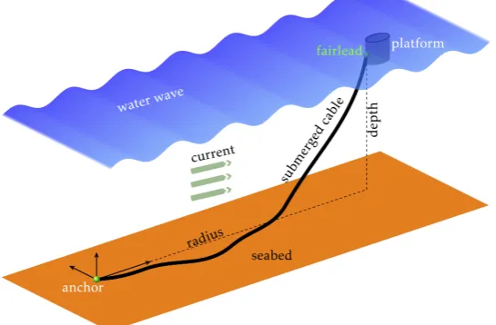
mooring force for given reference point motion of the platform. The program is based on the model of submerged cables, as in Figure 2, developed by [76–78], where the cable is modelled as an Euler beam considering the bending and torsional stiffness effects. The hydrodynamic effect is considered using the modified Morison’s equation. In the case that a part of the cable is grounded on the seabed, the seabed is considered as a flat plane modelled as a visco-elastic mattress. The stiffness of the seabed was taken from

190

the FAST [65] case files for the mooring system of the spar-type FOWT. According to the literature, the cable fairlead forces and hence the FOWT motion are not sensitive to the value of the stiffness. We have also performed a parametric analysis and confirmed that. The seabed stiffness is important if the focus is the fatigue analysis of the cable near the touchdown point. Using OpenMOOR, the fairlead motion is computed using the multi-body dynamics and then the two-point boundary problem for each cable is solved in parallel

195

using the generalized-αmethod for both spatial and temporal discretization [78]. The resulting nonlinear algebraic equation is eventually solved using a Newton-like method with dynamic relaxation. OpenMOOR also enables the consideration of steady current with an arbitrary profile. In the present study, the wave effect on the mooring cable is neglected since the fairleads of the spar-type FOWT are deep below the mean water level. For implementation, OpenMOOR is compiled as a dynamic linking library and then coupled

200

[image:7.595.162.435.345.524.2]

with the model of the FOWT. The coupling is achieved by returning the displacements and velocities of

Figure 2: Submerged cable subjected to wave and current

the platform reference point to OpenMoor and applying the obtained mooring loads to the platform. This creates one time step lag between the platform state and mooring loads. But, with sufficiently small time step this requirement can be waived and is the standard practise in state-of-the-art simulation tools like FAST [65].

205

2.3. Wave-current interaction model

The wave-current interaction is modelled using the Airy wave theory considering the effect of an under-lying current [79,80]. Two-dimensional flow is considered, i.e., the waves are travelling on a favourable and adverse current. For description of the flow field, a coordinate system is defined with the origin placed on the mean water level (MWL) withxthe horizontal axis andz the vertical axis pointing upwards.

210

2.3.1. Regular wave on current

(8)

uT(x, z, t) =U(z) +u(z) cos(κx−ωt) (8)

wT(x, z, t) =w(z) sin(κx−ωt) (9)

where U(z) is the current velocity varying with respect to z; and ω and κ denote the angular frequency and the wavenumber respectively. Note thatωis the apparent frequency with the current effect considered

215

[83]. In the preceding expressions,uT(x, z, t) andwT(x, z, t) are the flow velocities in horizontal and vertical directions, whileu(x, z, t) andw(x, z, t) are the wave velocities using the first-order term [81].

According to the Airy wave theory, the free surface elevationη is given as

η(x, t) =Acos(κx−ωt) (10)

where A = the surface wave amplitude. Given the free surface function, the flow velocity can be solved analytically for a uniform or linear current profile (d2_U_(z)/dz2_{= 0)(see [}₈₂_{] for details), as}

220

uT(x, z, t) =U(z) +A(ω−κU0)

cosh [κ(z+hw)] sinh(κhw)

cos(κx−ωt) (11)

wT(x, z, t) =A(ω−κU0)

sinh [κ(z+hw)] sinh(κhw)

sin(κx−ωt) (12)

whereU0= the current velocity atz= 0. The corresponding dispersion relation becomes

(ω−κU0)2=

gκ−(ω−κU0)

dU dz

tanh(κhw) (13)

which is valid for both uniform and linear shear currents. The solution of the preceding equation gives the wave numbers and the flow field is then explicitly determined using equations (11,12).

2.3.2. Irregular waves on current

To consider the current effect on irregular waves, the expressions in equations (11,12) are combined with

225

the spectral representation. The influence of the current on the wave spectrum is considered by [79]

S(ω, U) = 4S(ω)

1 +p1 + 4ωU/g

2

p

1 + 4ωU/g

(14)

whereS(ω, U) andS(ω) denote the wave spectra with and without an underlying current respectively. It is noted that whenω→ −g/4U, the wave components are unable to propagate against the current and wave breaking occurs and hence the preceding expression is only valid for 1 + 4ωU/g >0 if waves are travelling on an adverse current. To deal with the case when wave breaking happens, an “equilibrium limit” was defined

230

for deep water by [84,85] as

SER(ω, U) =

A∗g2

(ω−kU)5

1

1 + 2U(ω−κU)/g (15)

where the subscript ER refers to the equilibrium range and A∗ is a numerical constant in the range of 0.008–0.015 [86]. Equation 15is used instead for a given wave frequency whenever S(ω, U) is larger than SER(ω, U).

For irregular waves, the water surface elevation can be expressed as

η(x, t) = N

X

j=1

(9)

where φj is introduced as a random phase angle uniformly distributed from 0 to 2π and N denotes the number of wave components. The amplitude of thejth wave isAj=

p

2S(ωj, U)∆ωwith ∆ωthe frequency interval. Correspondingly, the flow velocities are given by

uT(x, z, t) =U(z) + N

X

j=1

Aj(ωj−κjU)

cosh [κj(z+hw)] sinh(κjhw)

cos(κjx−ωjt+φj) (17)

wT(x, z, t) = N

X

j=1

Aj(ωj−κjU)

sinh [κj(z+hw)] sinh(κjhw)

sin(κjx−ωjt+φj) (18)

The accelerations can be obtained from the preceding equations , as

235

˙

uT(x, z, t) = N

X

j=1

Ajωj(ωj−κjU)

cosh [κj(z+hw)] sinh(κjhw)

sin(κjx−ωjt+φj) (19)

˙

wT(x, z, t) =− N

X

j=1

Ajωj(ωj−κjU)

sinh [κj(z+hw)] sinh(kjhw)

cos(κjx−ωjt+φj) (20)

where the wave-number κj is solved from equation (13) for each wave component. An instance of the Pierson-Moskowitz spectrum with and without an underlying current is shown in Figure3. The parameters used are - significant wave height 10 m, peak spectral period 6 s and surface current velocity 0.609 m/s [87]. A decrease in the wave spectrum peak can be observed in the presence of an underlying current.

0 0.5 1 1.5 2 2.5

Wave frequency (rad/s) 0

1 2 3 4 5 6 7 8 9

Wave spectrum (m

2s/rad)

[image:9.595.189.403.425.602.2]

Without current With wave-current interaction

Figure 3: Pierson-Moskowitz spectrum with and without an underlying current

3. Multi-resolution wavelet-LQR pitch controller 240

(10)

reduced order system with four degrees of freedom (i.e., the three blade flapwise and tower fore-aft) are used. According to [61], a time-varying system can be represented as

˙

x(t) =A(t)x(t) +B(t)u(t) +F(t) (21)

with statesx∈ <n_{, control input}_u_{∈ <}m_{and external disturbance}_F_{∈ <}n_{. The reduced order time-varying} FOWT can be represented in this form, however, for controller design the closed form state-space equations are not required as will be shown subsequently. The state vector and control input vector are given as

x= [q, q˙]T, q= [qT F A1, qB1F1, qB2F1, qB3F1]

u= [β1, β2, β3]T

(22)

Wavelet transformation of equation 21 with respect to a basis function ψ with scale parameter a and translation parameterbleads to

W_ψ0

axi(b) =

n

X

k=1

Wψa(Aikxk)(b) +

m

X

k=1

Wψa(Bikuk)(b) +WψaFi(b) (23)

where prime denotes differentiation with respect to the translation parameterb and Wψa(·) is the wavelet

transformation of (·). Since, ψ[(t−b)/a] is a fast decaying function localized around t = b and Aik(t) & Bik(t) are slowing varying functions as compared to ψ[(t−b)/a] and xk(t); the wavelet transformation of the first two terms in the right hand side of equation23can be approximated as

Wψa(Aikxk)≈A0,ikWψaxk(b)

Wψa(Bikxk)≈B0,ikWψaxk(b)

(24)

where, A0 and B0 are the mean (nominal matrices) excluding the time varying components. Therefore,

equation23can be rewritten as W_ψ0

ax(b) =A0Wψax(b) +B0Wψau(b) +WψaF (25)

For the non-linear floating wind turbine system the linearised state matrixA0and linearised control influence

matrixB0 can be obtained from a Taylor series expansion till first order terms. The partial differentiations

can be performed using numerical central difference technique. For details on the form of the equations refer to [65]. For the system defined in equation25in wavelet domain the control input can be written in a state feedback form as

{Wψau}=−Ga{Wψax} (26)

where, Ga is scale parameter dependent gain matrix, i.e., a frequency band dependent gain matrix. With the control input of the above form a minimization cost functional can be defined as

Ja =

Z tc

t0

{Wψax}

T_Q

a{Wψax}+{Wψau}

T_R

a{Wψau} (27)

The definition of the cost function leads to the classical LQR problem for wavelet transformed states and control input. The weighting matricesQa, Ra are associated to the scaling parameter aand are specified for every frequency band.

Control input in time domain. The control input can be obtained in time domain by inverse wavelet trans-formation of the control input. The control input att=tc using the states from the interval [t0, tc] can be obtained as

u(tc) =−GLWψ−a1

Z aL

0

Z tc

t0

1

a2{Wψax(t)}ψ

_t

c−b a

dbda

− U

X

j=L+1

GjW_ψ−_a1

Z j+1

j

Z tc

t0

1

a2{Wψax(t)}ψ

_t

c−b a

dbda

(11)

where, the scaling parameter is discretized into bands{0, a1, a2, ... , aL, ..., aU, ...}. Where,aLis the lower threshold of frequency bands, aU is the upper is the upper threshold of frequency bands; and for higher

245

bandsaj> aU the control input is ignored.

Since continuous wavelet transform (CWT) is not suitable for synthesis of control input from time histories of finite interval, discrete wavelet transform (DWT) based on MRA is used for exact decomposi-tion/reconstruction of the signal. The filtered signal obtained from MRA is then used to obtain the control input in time domain as

u=−GL{x}L− U

X

j=L+1

Gj{x}j (29)

from frequency dependent control gains where,{x}L,{x}L+1, ...,{x}U are the filtered signal corresponding to discretized frequency bands. The frequency band dependent controller gains are estimated using different weighting matricesQjandRjfrom the solution of the Algebraic Riccati Equation (ARE) associated with the nominal state and control influence matricesA0 andB0. The wavelet-LQR controller is compared against

250

the classical LQR controller where the control input is estimated from gain scheduling of the unfiltered state and frequency band independent controller gain.

For every wind turbine the blade pitch angles, used as the control input, is limited by the pitching rate and maximum pitch angle that can be realized by the pitch actuators of the blades. Hence, the commanded pitch angles obtained from equation29are limited by maximum pitching rate of 8 degrees/sec and maximum

255

pitch angle of 90 degrees for the reference wind turbine [88].

4. Model verification results

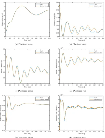
The offshore wind turbine model developed is benchmarked against state of the art wind turbine simulator FAST [65]. The spar-type offshore wind turbine defined in [88] is used for analysis. The codes for the offshore wind turbine are developed in MATLAB [89]. The verification results are shown in Figure4 and Figure 5.

260

The offshore wind turbine is simulated under steady rated wind speed of 11.4 m/s in still water.

An excellent similarity is observed for the wind turbine tower, nacelle and blade motion in Figure 4; while some dissimilarities are observed in the platform motion from Figure5. The main difference is a phase shift in the response time histories. This is due to the fact that while FAST applies hydrodynamic damping from both linear potential flow theory and viscous drag forces from Morison’s equation, the derived model in

265

this paper uses only viscous drag forces from Morison’s equation. This difference in hydrodynamic damping results in a phase shift in the response time histories. Also, the degrees of freedom that experience less hydrodynamic damping like platform surge, heave or reaches steady state quickly like platform pitch, yaw is less affected by the phase shift. The platform sway and roll degrees of freedom experience a noticeable phase shift due to the difference in hydrodynamic damping. However, the mean and the frequency content

270

of the responses remain the same which is important from a dynamic analysis point of view.

5. Controller performance evaluation

The non-linear aeroelastic offshore wind turbine model is used to simulate the dynamic behaviour of the spar-type floating offshore wind turbine. The different cases are simulated for a standard 600 sec and with a sampling rate of 40 Hz. Numerical Runga-Kutta method ‘ODE 4’ is used for time integration of

275

the non-linear system. The proposed controller is compared with a baseline PI collective pitch controller and a classical LQR pitch controller to illustrate the effectiveness of the proposed control strategy. The turbulent wind field is generated using the TurbSim[68] package distributed by NREL. It has the capability of generating turbulent 3-D wind field taking into account wind shear and spatial coherence. The turbulence in the wind has been assumed to be 10% in this paper. Two different wind cases are investigated here, i.e.,

280

(12)

0 20 40 60 80 100 120 140 160 180 200

Time (sec)

-1 0 1 2 3 4 5 6 7

Blade 1 out-of-plane displacement (m)

FAST Derived model

(a) Blade 1 out-of-plane displacement

0 20 40 60 80 100 120 140 160 180 200

Time (sec)

-1.4 -1.2 -1 -0.8 -0.6 -0.4 -0.2 0 0.2

Blade 1 in-plane displacement (m)

FAST Derived model

(b) Blade 1 in-plane displacement

0 20 40 60 80 100 120 140 160 180 200

Time (sec)

-0.1 0 0.1 0.2 0.3 0.4 0.5 0.6

Tower top fore-aft displacement (m)

FAST Derived model

(c) Tower top fore-aft displacement

0 20 40 60 80 100 120 140 160 180 200

Time (sec)

-0.1 -0.08 -0.06 -0.04 -0.02 0 0.02

Tower side-to-side displacement (m)

FAST Derived model

(d) Tower top side-to-side displacement

0 20 40 60 80 100 120 140 160 180 200

Time (sec)

-6 -4 -2 0 2 4 6 8

Nacelle yaw (degree)

10-3

FAST Derived model

(e) Nacelle yaw rotation

0 20 40 60 80 100 120 140 160 180 200

Time (sec)

10.6 10.8 11 11.2 11.4 11.6 11.8 12 12.2

Low speed shaft velocity (rpm)

FAST Derived model

[image:12.595.94.515.115.692.2]

(f) Low speed shaft speed

(13)

0 20 40 60 80 100 120 140 160 180 200

Time (sec)

-5 0 5 10 15 20 25 30 35

Platform Surge (m)

FAST Derived model

(a) Platform surge

0 20 40 60 80 100 120 140 160 180 200

Time (sec)

-0.4 -0.35 -0.3 -0.25 -0.2 -0.15 -0.1 -0.05 0 0.05

Platform Sway (m)

FAST Derived model

(b) Platform sway

0 20 40 60 80 100 120 140 160 180 200

Time (sec)

-1 -0.8 -0.6 -0.4 -0.2 0 0.2

Platform Heave (m)

FAST Derived model

(c) Platform heave

0 20 40 60 80 100 120 140 160 180 200

Time (sec)

-1 0 1 2 3 4 5 6 7

Platform Roll (radians)

10-3

FAST Derived model

(d) Platform roll

0 20 40 60 80 100 120 140 160 180 200

Time (sec)

-0.02 0 0.02 0.04 0.06 0.08 0.1 0.12

Platform Pitch (radians)

FAST Derived model

(e) Platform pitch

0 20 40 60 80 100 120 140 160 180 200

Time (sec)

-2 -1 0 1 2 3 4 5 6 7

Platform Yaw (radians)

10-3

FAST Derived model

[image:13.595.90.519.115.679.2]

(f) Platform yaw

(14)

period is assumed to be 6 s for all simulations. The depth-dependent wave velocity and accelerations are obtained from equations17,18,19 and 20with underlying current. The offshore wind turbine is simulated

285

without current and with an underlying current of uniform and linear profile. The surface current velocity is assumed to be 0.609 m/s [87] in the along wind direction, which is the same as the wave propagation direction. The above sea-states represent a violent ocean. For illustration purposed, the controller performance is also evaluated under moderate sea-states ofHs= 2.25m andTp= 6.25s and presented here.

The proposed pitch controller is employed in the FOWT and simulated under the above mentioned

met-290

ocean conditions. Its performance is compared against the baseline pitch controller and the classical LQR controller. The three controllers used are defined as follows:

1. Baseline controller. The baseline controller is described in [91] which also provides the FORTRAN source code for the control algorithm. The same was rewritten in MATLAB[89] with changes prescribed in [88].

295

2. LQR controller. The LQR pitch controller is designed using state weight matrixQ= 5×Iand input weight matrixR= 15000×Ifor 14 m/s wind speed andQ= 300×IandR= 15000×Ifor 25 m/s wind speed. The weights are chosen a-priori after a few trial and errors to optimize the effort between the response states and pitch angles.

3. Wavelet-LQR controller (W-LQR).The advantage of the wavelet-LQR controller is that it is capable

300

of applying different weights to different frequency bands. For that purpose, the signal from a finite internal [t0 tc] is filtered using ‘db6’ wavelet from the Daubechies wavelets [92]. The response is decomposed into 5 levels, where for a response sampled at 40 Hz, the reconstructed approximate signal at 5th _{level contains frequencies in the band [0 Hz 1.2 Hz]. This band contains the frequencies}

that are required to be suppressed, i.e., the rotational frequency of the wind turbine and the blade’s

305

natural frequency. Hence, the 5th_{band becomes the lower bound where additional emphasis is placed}

on the response states by relaxing the control weight of this band to RL = 3000×I. All other parameters remain the same. Also, reconstructed detailed signals from levels 1 and 2 are disregarded in the estimation of control input.

5.1. Reference wind speed 14 m/s without underlying current

310

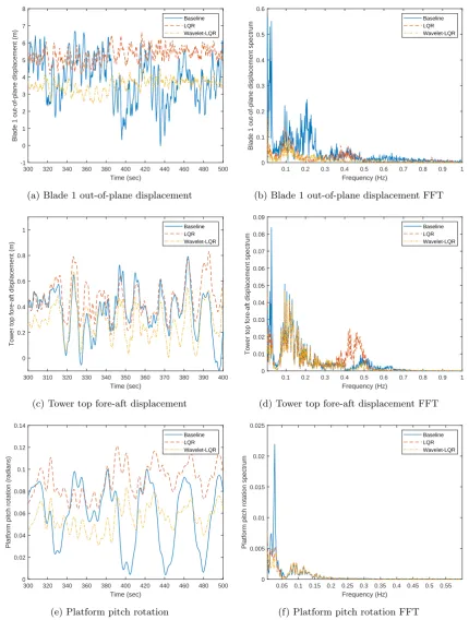
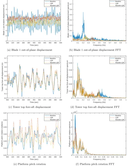
The responses of the offshore wind turbine using the three different controllers and without any underlying current is shown in Figure 6. It can be observed from Figure 6(a) that excellent vibration reduction is obtained using the proposed wavelet controller for the blade out-of-plane motion. The LQR controller is capable of reducing the amplitude of the response but the peaks of the response are similar to that of the baseline controller. The corresponding Fourier spectrum of the response in Figure6(b) shows that the

315

1P rotational frequency i.e., 0.2 Hz has been effectively suppressed by the proposed controller. It is also interesting to note that the two visible peaks below 0.2 Hz in the blade out-of-plane response spectrum is the effect of dynamic coupling between the blade-tower-platform. The response of the blade is heavily affected by the pitching motion of the platform and the fore-aft motion of the tower. However, the proposed controller is capable of suppressing these two peaks very effectively. Although the LQR controller is capable

320

of mitigating these response frequencies, the wavelet-LQR controller performs better as is shown in the figures.

The tower fore-aft motion is shown in6(c) with its Fourier spectrum in6(d). Again, the wavelet-LQR controller performs significantly better than the baseline controller and LQR controller as can be observed from the time history. While the wavelet-LQR is capable of suppressing the various frequency peaks, the

325

LQR controller is only capable of suppressing the lower frequency peak and higher peaks are observed in the higher frequency range. The response time history shows that, with the LQR controller, the response peaks are of greater amplitude than when the baseline controller is used.

Finally, the platform pitching motion is shown in 6(e) with its Fourier spectrum in 6(f). It can be observed that the pitching motion is dominated by a single frequency and it is mitigated effectively by the

330

(15)

300 320 340 360 380 400 420 440 460 480 500

Time (sec)

-1 0 1 2 3 4 5 6 7 8

Baseline LQR Wavelet-LQR

0.1 0.2 0.3 0.4 0.5 0.6 0.7 0.8 0.9 1

Frequency (Hz)

0 0.1 0.2 0.3 0.4 0.5 0.6

Blade 1 out-of-plane displacement spectrum

(b) Blade 1 out-of-plane displacement FFT

300 310 320 330 340 350 360 370 380 390 400

Time (sec)

0 0.2 0.4 0.6 0.8 1

0.1 0.2 0.3 0.4 0.5 0.6 0.7 0.8 0.9 1

Frequency (Hz)

0 0.01 0.02 0.03 0.04 0.05 0.06 0.07 0.08 0.09

Tower top fore-aft displacement spectrum

(d) Tower top fore-aft displacement FFT

300 320 340 360 380 400 420 440 460 480 500

Time (sec)

0 0.02 0.04 0.06 0.08 0.1 0.12 0.14

Platform pitch rotation (radians)

(e) Platform pitch rotation

0.05 0.1 0.15 0.2 0.25 0.3 0.35 0.4 0.45 0.5 0.55

Frequency (Hz)

0 0.005 0.01 0.015 0.02 0.025

Platform pitch rotation spectrum

[image:15.595.87.518.116.685.2]

(f) Platform pitch rotation FFT

(16)

300 320 340 360 380 400 420 440 460 480 500

Time (sec)

0 1 2 3 4 5 6 7 8

0.1 0.2 0.3 0.4 0.5 0.6 0.7 0.8 0.9 1

Frequency (Hz)

0 0.1 0.2 0.3 0.4 0.5 0.6

300 310 320 330 340 350 360 370 380 390 400

Time (sec)

0 0.2 0.4 0.6 0.8 1 1.2

0.1 0.2 0.3 0.4 0.5 0.6 0.7 0.8 0.9 1

Frequency (Hz)

0 0.01 0.02 0.03 0.04 0.05 0.06 0.07

300 320 340 360 380 400 420 440 460 480 500

Time (sec)

0 0.02 0.04 0.06 0.08 0.1 0.12 0.14

0.05 0.1 0.15 0.2 0.25 0.3 0.35 0.4 0.45 0.5 0.55

Frequency (Hz)

0 0.002 0.004 0.006 0.008 0.01 0.012 0.014 0.016 0.018 0.02

[image:16.595.92.519.118.684.2]

(17)

5.2. Reference wind speed 14 m/s with underlying current of uniform profile

The offshore wind turbine is simulated next with an underlying current of a uniform profile at the same hub-height reference wind speed of 14 m/s and the performance of the three different pitch controllers is

335

compared in Figure7. The response time histories, Fourier spectrum and controller performance are almost identical to that when the offshore wind turbine is simulated without the underlying current. The same conclusion can be made about the controller performance and is therefore not repeated. The only difference that can be observed is that the Fourier spectrum amplitudes are fractionally reduced. This is due to the fact that the underlying current decreases the wave turbulence as can be observed from the reduced peak of

340

the wave spectrum in Figure3 in the presence of an underlying current. Although this underlying current has negligible impact on the wind turbine degrees of freedom, the dynamic behaviour of the platform surge motion is heavily affected as shown in Figure 9. The current, when in the same direction as that of the wave, increases the platform surge motion. It can be also observed from Figure9that the underlying current reduces that turbulence in the surge motion of the platform. Since the dynamics of the surge motion much

345

slower than the other components, it behaves as a static offset in the position of the wind turbine without any significant effect on the dynamics of the wind turbine and the performance of the controller.

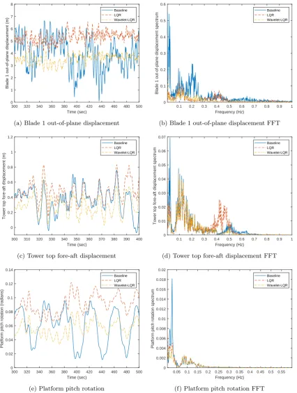
5.3. Reference wind speed 25 m/s with underlying current of linear profile

In this case, the performance of the three controllers is compared at a reference wind speed of 25 m/s with an underlying current of a linear profile. The response time histories for the along-wind components along

350

with their Fourier spectrum is shown in Figure8. Again, a considerable reduction in blade out-of-plane using the proposed controller can be observed in Figure8(a) and the peak associated with the 1P frequency of the wind turbine is clearly seen to be suppressed in Figure8(b). It can be again observed that the proposed wavelet-LQR controller performs better than the baseline controller and the LQR pitch controller. Further reduction in the tower fore-aft motion and the platform pitching motion using the wavelet-LQR controller is

355

observed where the LQR pitch controller shows poor performance. The decrease in the response spectrum amplitudes of the tower fore-aft motion in Figure8(d) and platform pitching motion in Figure8(f) illustrates that the proposed controller is capable of mitigating the tower and the platform pitching motions through load reduction.

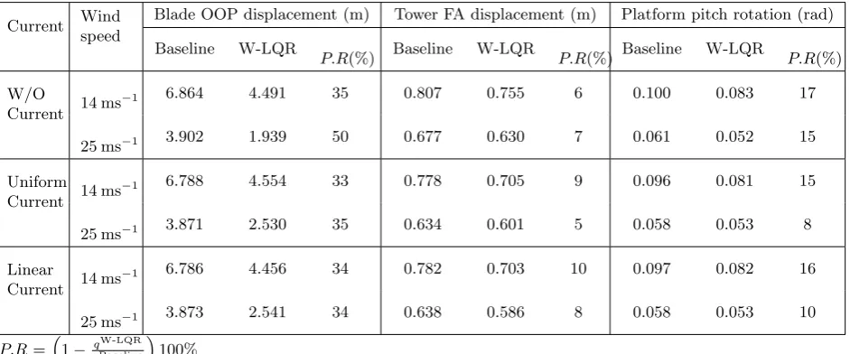
Tables 1 and 2 show the peak and the standard deviation of the blade, tower and platform motion

360

associated with the baseline and the proposed Wavelet-LQR pitch controllers at the various met-ocean conditions considered in this paper. The percentage reduction over the baseline controller is also shown in the tables. The choice of the two wind speeds is based on the fact that, it lies at the bounds of region 3 of operational wind speeds. It has been shown that the response peaks and standard deviations are reduced with the proposed wavelet-LQR controller in both cases. A considerable reduction is obtained at 14 m/s

365

wind speed with the different current profiles. The results presented in Tables1and2show that at the cut-out wind speed of 25 m/s the performance of the proposed controller in mitigating the standard deviation of the responses drop slightly but promising reductions in response peaks are still observed. No significant difference in the controller performance is observed under different current profiles.

It has been shown the emphasis on 1P rotational frequency reduces the aerodynamic load associated

370

with it and results in reduced pitching motion of the platform. However, this reduction of aerodynamic loads provides additional benefit in the form of reduced in-plane motion of the wind turbine which is not the objective of the controller. The blade in-plane motion, tower side-to-side motion, rotor speed and platform roll of the floating wind turbine for 14 m/s and 25 m/s are shown in Figure10and Figure11respectively. It can be observed that compared to the baseline controller the proposed wavelet-LQR controller is capable of

375

reducing the structural vibrations by reducing the aerodynamic loads associated with 1P frequency. Further, the platform roll is also reduced thanks to the reduced load on the wind turbine. The reduction in platform pitch and roll establishes the fact that the proposed control not only ensures stability of the entire floating wind turbine but also reduces the rotation of the platform which is beneficial for power production.

It can also be observed from Figure 10(c) and Figure 11(c) that the variability in the rotor speed

380

(18)

300 320 340 360 380 400 420 440 460 480 500

Time (sec)

-3 -2 -1 0 1 2 3 4 5

0.1 0.2 0.3 0.4 0.5 0.6 0.7 0.8 0.9 1

Frequency (Hz)

0 0.1 0.2 0.3 0.4 0.5 0.6 0.7 0.8

300 310 320 330 340 350 360 370 380 390 400

Time (sec)

-0.2 -0.1 0 0.1 0.2 0.3 0.4 0.5 0.6 0.7

0.1 0.2 0.3 0.4 0.5 0.6 0.7 0.8 0.9 1

Frequency (Hz)

0 0.01 0.02 0.03 0.04 0.05 0.06

300 320 340 360 380 400 420 440 460 480 500

Time (sec)

0.01 0.02 0.03 0.04 0.05 0.06 0.07

0.05 0.1 0.15 0.2 0.25 0.3 0.35 0.4 0.45 0.5 0.55

Frequency (Hz)

0 1 2 3 4 5 6

10-3

[image:18.595.88.515.128.684.2]

(19)

0 100 200 300 400 500 600

Time (sec)

-5 0 5 10 15 20 25 30 35

Platform Surge (m)

No current Uniform current Linear current

(a) Reference wind speed 14 m/s

0 100 200 300 400 500 600

Time (sec)

0 2 4 6 8 10 12 14 16 18 20

Platform Surge (m)

No current Uniform current Linear current

[image:19.595.97.517.118.295.2]

(b) Reference wind speed 25 m/s

Figure 9: Static offset created by the underlying current

Table 1: Peak response magnitudes using the three different controllers

Current Wind speed

Blade OOP displacement (m) Tower FA displacement (m) Platform pitch rotation (rad)

Baseline W-LQR

P.R(%) Baseline W-LQR P.R(%) Baseline W-LQR P.R(%)

W/O

Current 14 ms

−1 6.864 4.491 35 0.807 0.755 6 0.100 0.083 17

25 ms−1 3.902 1.939 50 0.677 0.630 7 0.061 0.052 15

Uniform Current 14 ms

−1 6.788 4.554 33 0.778 0.705 9 0.096 0.081 15

25 ms−1 3.871 2.530 35 0.634 0.601 5 0.058 0.053 8

Linear

Current 14 ms

−1 6.786 4.456 34 0.782 0.703 10 0.097 0.082 16

25 ms−1 3.873 2.541 34 0.638 0.586 8 0.058 0.053 10

P.R=1− qW-LQR qBaseline

100%

rpm, the Wavelet-LQR controller is designed to reduce structural vibrations. The LQR gains are selected appropriately to keep the rotor speed around the rated value while aiming for greater load reduction. In this study, it has been found the standard deviation of the low-speed-shaft/rotor speed from 12.1 rpm using the

385

baseline PI controller is 1.21 rpm and 1.40 rmp for wind speeds of 14 m/s and 25 m/s respectively. For the proposed Wavelet-LQR controller the standard deviations of the rotor speed for the respective wind speeds are 1.72 rpm and 1.87 rmp. While there is an increase in the standard deviation, the coefficient of variation in the worst scenario is still under 15 %. Also, as pointed out by [62, 93], individual wind turbine power variability will be less important as an offshore wind turbine will almost certainly be situated in a large

390

wind farm and the total output of the farm will be predominantly dictated by the spatial and temporal variations of the farm rather than the variability of a single turbine. Hence, this increase in individual wind turbine power variability is judged to be acceptable considering the promising reduction in structural loads. This trade-off between structural response mitigation and rotor speed maintenance can prove to be beneficial in extending the design life of the wind turbine components. It must be noted here that the

[image:19.595.67.538.351.547.2]

(20)

[image:20.595.63.539.128.299.2]

Table 2: Response standard deviations using the three different controllers

Current Wind speed (m/s)

Blade OOP disp. (m) Tower FA disp. (m) Platform pit. rot. (rad) Rotor speed (rpm)

Base-line

W-LQR

P.R (%)

Base-line

W-LQR

P.R (%)

Base-line

W-LQR

P.R (%)

Base-line

W-LQR

W/O Current

14 1.212 0.320 74 0.161 0.124 23 0.023 0.011 54 1.21 1.72

25 1.099 0.404 63 0.140 0.126 10 0.011 0.008 25 1.40 1.87

Uniform Current

14 1.176 0.316 73 0.150 0.117 22 0.020 0.010 52 1.19 1.70

25 1.092 0.392 64 0.130 0.119 8 0.009 0.008 15 1.39 1.83

Linear Current

14 1.183 0.316 73 0.151 0.117 23 0.021 0.010 52 1.20 1.71

25 1.091 0.388 64 0.130 0.118 9 0.009 0.007 18 1.40 1.86

P.R=1− qW-LQR qBaseline

100%

controller is designed with the primary aim of vibration control and rotor speed regulation is not included. In principle, increasing the weight on the states, or conversely decreasing the weight on the control input, will improve vibration control. However, this is at a cost of increased pitch actuation and rotor speed variability. In this paper, the weights are selected so that excellent vibration control is achieved at a cost of slightly increased rotor speed error. The authors would to point out here that it is possible to reduce rotor speed

400

error by sacrificing on vibration control. The controller weight matrices are design parameters that can be determined based on the requirement. Another important aspect of the controller design is the pitching rate of the blades which demonstrates the rate of use of pitch actuators. It has been observed that the maximum pitch rate for the baseline PI pitch controller is 1.63 deg/s and 0.42 deg/s for wind speeds of 14 m/s and 25 m/s respectively. However, with the Wavelet-LQR pitch controller the maximum pitch rate is saturated

405

at 8 deg/s which is the design specification. Hence, the improved structural response if obtained from an increased use of pitch actuation.

Lastly, as it was mentioned before the proposed controller is compared against the baseline controller at a hub height wind speed of 14 m/s, moderate sea-states and an underlying current of linear profile and is shown in Figure12and Figure13. A similar observation can be made about the controller performance

410

where a significant reduction in structural responses is achieved at a cost of increased rotor speed variability. The pitch and roll of the platform are reduced while the rotor speed still tracks the rated value. As mentioned earlier this increase in variability is judged to be acceptable given the significant amount of reduction in structural responses that is achieved.

6. Conclusion 415

This paper proposes the use of a wavelet-LQR based individual pitch controller for response mitigation and load reduction in spar-type floating offshore wind turbines considering wave-current interactions. A reduced order model using the blade out-of-plane and tower fore-aft degrees of freedom is used to develop the controller. The proposed wavelet-LQR controller has the capability of assigning frequency band dependent LQR gains. This capability has been used in this study to emphasize on the 1P frequency of the wind

420

turbine along with the blade out-of-plane natural frequency. The controller is compared against the baseline controller and the classical LQR controller. The numerical results presented in this paper show that the wavelet-LQR controller perform better than the baseline controller and the LQR controller for different met-ocean conditions in reducing structural loads. The wind speeds are selected so that they lie on the bound of region 3 of operational wind speeds. The performance at the two different wind speeds shows that

425

(21)

300 320 340 360 380 400 420 440 460 480 500

Time (sec)

-2 -1.5 -1 -0.5 0 0.5

Baseline Wavelet-LQR

(a) Blade in-plane displacement

300 320 340 360 380 400 420 440 460 480 500

Time (sec)

-0.1 -0.09 -0.08 -0.07 -0.06 -0.05 -0.04 -0.03 -0.02 -0.01

(b) Tower side-to-side displacement

0 100 200 300 400 500 600

Time (sec)

9 10 11 12 13 14 15 16 17

Rotor Speed (RPM)

(c) Low speed shaft/rotor speed

0 100 200 300 400 500 600

Time (sec)

-2 0 2 4 6 8 10 12

10-3

[image:21.595.93.517.121.493.2]

(d) Platform roll

Figure 10: Hub height reference wind speed 14 m/s and underlying current of linear profile

better performance than the baseline controller is obtained in full range of wind speeds. The emphasis on the 1P frequency of the wind turbine reduces the aerodynamic loads which in turn reduces vibration in tower fore-aft and platform pitching motion of the wind turbine. It has been shown that the pitching of the platform contributes significantly to the dynamics of the blade and the tower. However, the proposed

430

controller is capable of minimizing the pitching motion of the platform together with the blade out-of-plane motion and tower fore-aft motion. Additional benefit is achieved in the form of reduction of blade in-plane motion, tower side-to-side motion and platform roll that arises from aerodynamic load reduction associated with the 1P frequency of the wind turbine. The proposed controller not only ensures the stability of the entire wind turbine but also reduces the platform pitch and roll. It has been observed that this improved

435

structural response is obtained at a cost of increased use of pitch actuation. It has also been shown that the improved structural response of the offshore wind turbine results in an increase in deviation from the rate rotor speed which leads to increased power variability. However, as has been mention in the previous section the significance of this individual wind turbine power variability will be further minimized when an entire wind farm is considered. This trade-off between vibration reduction and rotor speed improvement

440

can prove to be beneficial in increasing the design life of the wind turbine components.

(22)

300 320 340 360 380 400 420 440 460 480 500

Time (sec)

-2 -1.5 -1 -0.5 0 0.5 1 1.5

(a) Blade in-plane displacement

300 320 340 360 380 400 420 440 460 480 500

Time (sec)

-0.18 -0.16 -0.14 -0.12 -0.1 -0.08 -0.06 -0.04 -0.02 0 0.02

(b) Tower side-to-side displacement

0 100 200 300 400 500 600

Time (sec)

8 10 12 14 16 18 20 22

Rotor Speed (RPM)

(c) Low speed shaft/rotor speed

0 100 200 300 400 500 600

Time (sec)

-0.015 -0.01 -0.005 0 0.005 0.01 0.015 0.02 0.025

[image:22.595.90.514.112.498.2]

(d) Platform roll

Figure 11: Hub height reference wind speed 25 m/s and underlying current of linear profile

effect on the performance of the controller. The results presented also show the importance of wave-current interaction on offshore wind turbines. The effect of vorticity in presence of ocean currents can generate complex fluid motion [94, 95]. The dynamics of the spar can be significantly affected by the presence of

445

vorticity [96–98] which requires further investigation and will be addressed in future works.

Acknowledgement

The second author, L. Chen, is supported by the Irish Research Council through the Government of Ireland Postdoctoral Fellowship (Project ID: GOIPD/2017/1260), which is gratefully acknowledged.

Appendix A. 450

(23)

100 150 200 250 300 350 400 450 500 550 600

Time (sec)

0 1 2 3 4 5 6 7

(a) Blade out-of-plane displacement

100 150 200 250 300 350 400 450 500 550 600

Time (sec)

-1.6 -1.4 -1.2 -1 -0.8 -0.6 -0.4 -0.2 0 0.2

(b) Blade in-plane displacement

200 250 300 350 400 450 500

Time (sec)

0 0.1 0.2 0.3 0.4 0.5 0.6 0.7

200 250 300 350 400 450 500

Time (sec)

-0.12 -0.1 -0.08 -0.06 -0.04 -0.02 0

(d) Tower top side-to-side displacement

100 150 200 250 300 350 400 450 500 550 600

Time (sec)

0 0.02 0.04 0.06 0.08 0.1 0.12

(e) Platform pitch

100 150 200 250 300 350 400 450 500 550 600

Time (sec)

-2 0 2 4 6 8 10 12

10-3

[image:23.595.90.519.108.691.2]

(f) Platform Roll

(24)

0 100 200 300 400 500 600 Time (sec)

9 10 11 12 13 14 15 16 17

Rotor Speed (RPM)

[image:24.595.188.404.119.298.2]

Figure 13: Rotor speed at wind speed 14 m/s and underlying current of linear profile and moderate sea states

qSg Platform surge qSw Platform sway qHv Platform heave qR Platform roll qP Platform pitch

qY Platform yaw

qT F A1 First tower fore-aft bending mode

qT F A2 Second tower fore-aft bending mode

qT SS1 First tower side-to-side bending mode

qT SS2 Second tower side-to-side bending mode

qyaw Nacelle yaw

qGeAz Generator azimuth angle qDrT r Drive-train torsional flexibility

qBiF1 First flapwise bending mode forithblade

qBiF2 Second flapwise bending mode forithblade

qBiE1 First edgewise bending mode forithblade

References

[1] Lackner, M.A.. Controlling platform motions and reducing blade loads for floating wind turbines. Wind Engineering 2009;33(6):541–553.

[2] Lackner, M.A., Rotea, M.A.. Passive structural control of offshore wind turbines. Wind energy 2011;14(3):373–388. 455

[3] Staino, A., Basu, B., Nielsen, S.R.. Actuator control of edgewise vibrations in wind turbine blades. Journal of Sound and Vibration 2012;331(6):1233–1256.

[4] Fitzgerald, B., Basu, B., Nielsen, S.R.. Active tuned mass dampers for control of in-plane vibrations of wind turbine blades. Structural Control and Health Monitoring 2013;20(12):1377–1396.

[5] Dinh, V.N., Basu, B.. Passive control of floating offshore wind turbine nacelle and spar vibrations by multiple tuned 460

mass dampers. Structural Control and Health Monitoring 2015;22(1):152–176.

[6] Hemmati, A., Oterkus, E., Barltrop, N.. Fragility reduction of offshore wind turbines using tuned liquid column dampers. Soil Dynamics and Earthquake Engineering 2019;125:105705.

[7] Basu, B., Zhang, Z., Nielsen, S.R.. Damping of edgewise vibration in wind turbine blades by means of circular liquid dampers. Wind Energy 2016;19(2):213–226.