Numerical Experiments Using MATLAB: Superconvergence of Conforming Finite, Element Approximation for Second Order, Elliptic Problems

ISSN Print: 2152-7385

DOI: 10.4236/am.2018.96047 Jun. 29, 2018 691 Applied Mathematics

Numerical Experiments Using MATLAB:

Superconvergence of Conforming Finite,

Element Approximation for Second Order,

Elliptic Problems

Anna Harris

1*

, Stephen Harris

2

, Camille Gardner

1

, Tyrone Brock

1

1_{Department of Mathematics and Computer Science, University of Arkansas at Pine Bluff, Pine Bluff, USA} 2_{US Food and Drug Administration, National Center for Toxicology Research,Jefferson, USA}

Abstract

The superconvergence in the finite element method is a phenomenon in which the finite element approximation converges to the exact solution at a rate higher than the optimal order error estimate. Wang proposed and ana-lyzed superconvergence of the conforming finite element method by L2_{-projections. The goal of this paper is to perform numerical experiments}

using MATLAB to support and to verify the theoretical results in Wang for the superconvergence of the conforming finite element method (CFEM) for the second order elliptic problems by L2_{-projection methods. MATLAB codes}

are published at https://github.com/annaleeharris/Superconvergence-CFEM for anyone to use and to study.

Keywords

Conforming Finite Element Methods, Superconvergence, L2_-Projection,

Second Order Elliptic Equationm, MATLAB

1. Introduction

Finite element method (FEM) is based on the premise that an approximation to any complex engineering problem can be reached by subdividing the problem into smaller and more manageable elements. Using FEMs partial differential equations that describe the behavior of structures can be reduced to a set of li-near equations that can easily be solved using the standard techniques of matrix algebra. FEM is used in virtually every engineering discipline. The aerospace, automotive, biomedical, chemicals, electronics, energy, geotechnical,

manufac-How to cite this paper: Harris, A., Harris, S., Gardner, C. and Brock, T. (2018) Nu-merical Experiments Using MATLAB: Superconvergence of Conforming Finite, Element Approximation for Second Order, Elliptic Problems. Applied Mathematics, 9, 691-701.

https://doi.org/10.4236/am.2018.96047

Received: January 25, 2018 Accepted: June 26, 2018 Published: June 29, 2018

Copyright © 2018 by authors and Scientific Research Publishing Inc. This work is licensed under the Creative Commons Attribution International License (CC BY 4.0).

http://creativecommons.org/licenses/by/4.0/

DOI: 10.4236/am.2018.96047 692 Applied Mathematics turing, and plastics industries routinely apply finite element analysis. In addi-tion, it is used not only for analyzing classical static structural problems, but also for such diverse areas as mass transport, heat transfer, dynamics, stability, and radiation problems.

The main objective of the superconvergence using various FEMs is to improve the accuracy of the existing approximation solution by applying certain post-processing techniques that are easy to implement. To obtain the supercon-vergence of FEMs, several methods have been proposed in the literature in the last thirty years. The method of local averaging has been a popular and useful technique in the study of superconvergence [1]-[9]. The underlying assumption of the existing superconvergence technique is that the finite element mesh has some special properties such as uniformity [7], local point-symmetry [8] [10], local translation-invariance [1][8], or orthogonality [5][11][12][13].

Zienkiewicz and Zhu [14][15] introduced the patch recovery technique which provides some superconvergence for the gradient of the finite element solution by using a discrete least-squares fitting on a local patch with high order polyno-mials. The method of Zienkiewicz and Zhu has been computationally proved to be robust and efficient and to produce some superconvergence for the gradient of the finite element solution.

Wang proposed and analyzed superconvergence of the conforming finite ele-ment method (CFEM) by L2_{-projections. The main idea behind the L}2_-projections

is to project the finite element solution to another finite element space with a coarse mesh and a higher order of polynomials.

The objective of this paper is to investigate the theoretical results in [16] for the conforming finite element approximations for second-order elliptic prob-lems by L2_{-projection methods and to support the theoretical results with}

nu-merical experiments using MATLAB.

This paper is organized as follows. In Section 2, we present a review for the conforming finite element method for the second-order elliptic problem. In Sec-tion 3, we investigate the theoretical results in [16], the superconvergence of CFEM for the second-order elliptic problem by L2_{-projection methods. In}

sec-tion 4, we perform numerical experiments to support the theoretical results in [16]. Numerical experiments of superconvergence of CFEM are performed in MATLAB and its codes are posted at

https://github.com/annaleeharris/Superconvergence-CFEM for anyone to use

and to study.

2. CFEM for the Second-Order Elliptic Problem

Consider the second-order elliptic problem with the homogeneous Dirichlet boundary condition which seeks _{u H∈} 1

( )

_{Ω satisfying}

in , 0 on ,

u f u

∆ = Ω

= ∂Ω (1)

DOI: 10.4236/am.2018.96047 693 Applied Mathematics subset of R2_{, ∂Ω is a Lipschitz continuous boundary, and a given function f is}

the external force.

A variational formulation of (1) seeks 1

( )

0

u H∈ Ω _{such that}

( ) (

)

1

( )

0

, , , ,

a u v = f v ∀ ∈v H Ω ₍₂₎

where

( ) (

, ,

)

d

a u v = ∇ ∇ = ∇ ⋅∇ Ωu v

_∫

_Ω u v

Let h be a quasi-uniform, i.e., it is regular and satisfies the inverse assump-tion [17], triangulation of Ω with

diam K

( )

≤

h K

,

∈



_h and let

P K

r

( )

be the space of polynomials of degree at most r with r≥0 _{on K. Assume that the} polynomial space in the construction of Vh contains

P K k

k

( )

,

≥

1

. Define the finite element space Vh associated with h as

( )

( )

{

1

}

0 : , .

h K k h

V = ∈v H Ω v ∈P K ∀ ∈K 

The finite element space Vh is assumed to satisfy the following approxima-tion property for any _{u H∈} m+1

( )

_Ω

:

(

)

1

1 1

inf , 0 .

h

m m

v V u v h u v Ch u m k

+ +

∈ − + − ≤ ≤ ≤ (3)

The finite element approximation problem (2) seeks u Vh∈ h such that

(

_h

,

) ( )

, ,

_h

,

a u v

=

f v

∀ ∈

v V

₍₄₎ where

(

h,

) (

h,

)

h d .

a u v = ∇ ∇ = ∇ ⋅∇u v

_∫

_Ω u v x

A well known error estimate for the finite element approximation solution h

u is the following:

1

1 inf_h ,

h _{v V}

u u C u v

∈

− ≤ − (5)

where C is a constant independent of the mesh size h.

Then from (3) and (5) we arrive at the following error estimate:

1

1 .

k

h k

u u− ≤Ch u ₊

To apply the superconvergence of finite element approximation, we assume that domain Ω is so regular that it ensures a

_{H s}

s

,

_≥

1

_{, regularity for the} solu-tion of (2). In other words, for any _{f H∈} s−2

( )

_Ω

the problem (2) has a unique solution 1

( )

0

u H∈ Ω _{satisfying the following a priori estimate:}

( )

2

2, s , 1.

s s

u C f f H − s

−

≤ ∀ ∈ Ω ≥ ₍₆₎

where C is a constant independent of data g.

3. Superconvergence of CFEM

Let τ be another finite element partition with coarse mesh size τ where hτ. Assume that τ and h have the following relation:

( )

, 0,1 .

hα

τ

=

α

∈

de-DOI: 10.4236/am.2018.96047 694 Applied Mathematics gree r associated with the partition τ. Define Qτ to be the L2-projection from

( )

2

L Ω _{onto the finite element space} Vτ. The finite element space Vτ is de-fined by

( )

( )

{

2 _{: ,}

}

_.

r K

Vτ = ∈v L Ω v ∈P K ∀ ∈K τ

For the superconvergence of CFEM, the following theoretical results can be found in [16].

Lemma 1 Assume that the second-order elliptic problems (2) holds (6) with 1≤ ≤ +s k 1 _and Vτ ⊂Hs−2

( )

Ω . Then there exists a constant C independent of h and τ such that

1,

h h

Q u Q u Ch u uσ

τ − τ ≤ − (7)

where

σ

= − +

s

1

α

min 0,2

(

−

s

)

,

α

∈

( )

0,1

_and τh.

Theorem 1 Assume that (6) holds true with 1≤ ≤ +s k 1 and

( )

2

s

Vτ ⊂H − Ω . If

u u x y

h

=

h

( )

,

is the finite element approximation of the exact solution

u u x y

=

( )

,

_{of (2), then there exists a constant C independent of h and} τ such that

( )1

1 1,

r k

h r k

u Q u Chα u Ch σ u

τ + + + +

− ≤ + ₍₈₎

where

σ

= − +

s

1

α

min 0,2

(

−

s

)

_.

Theorem 2 Assume that (6) holds true with 1≤ ≤ +s k 1 and

( )

2

s

Vτ ⊂H − Ω . If uh is the finite element approximation of the exact solution

( )

( )

( )

1 1 1

0

k r

u H_∈ + _{Ω }H + _{Ω }H _{Ω of (2), then there exists a constant C} inde-pendent of h and τ such that

(

)

r ₁ k ₁,

h _{r k}

u Q u Ch uα Ch σ α u

τ ₊ + − ₊

∇ − ≤ + ₍₉₎

where

σ

= − +

s

1

α

min 0,2

(

−

s

)

_.

From (8) and (9) α is selected to optimize the error estimates:

(

1

)

. 1 min 0,2

k s

r s

α= + −

+ − − (10)

4. Numerical Experiments of Superconvergence of CFEM by

L

2

_{-Projection Methods}

In this section, we confirm the theoretical results in [16] with numerical experi-ments for second-order elliptic problems. Assume that the exact solution of the second-order elliptic problem has _Hs _{regularity for some 1≤ ≤s 2 and for} simplicity, assume k=1, s=2_{, and} r=2 which gives 2

3

α= using the α Formula (10).

Then according to the theoretical results in [16], the best possible error esti-mates using the results (8) and (9) are given by

( )1 1 min 0,2( ) 2

1 1 3

r k s s

h r k

u Q u Chα u Ch α u Ch u

τ + + + − + − +

− ≤ + ≤ ₍₁₁₎

and

(

)

1 min 0,2( ) 4₃

1 1 3.

k s s

r

h r k

u Q u Ch uα Ch α α u Ch u

τ + + − − + − +

DOI: 10.4236/am.2018.96047 695 Applied Mathematics From the result (11), we do not see any superconvergence in L2 _norm.

How-ever, from the result (12), we have some superconvergence for the gradient error estimate.

The finite element partition h is constructed by dividing the domain into an _{n n}3_× 3 _{rectangular mesh then dividing the rectangular mesh with the}

posi-tive slope to form two triangles. The coarse finite element partition τ is also constructed by dividing the domain into an _{n n}2_× 2 _{rectangular mesh then}

di-viding the rectangular mesh with the positive slope to form two triangles. The finite element space Vh consists of the space of the linear polynomials

P K

1

( )

associated with the partition h and the dual finite element space Vτ consists of the space of the quadratic polynomials

P K

2

( )

associated with the partition

τ

 . The finite element spaces Vh and Vτ are defined by

( )

( )

{

1

}

0 : 1 ,

h K h

V = ∈v H Ω v ∈P K ∀ ∈K _

and

( )

( )

{

2

}

2

: _K , .

Vτ = ∈v L Ω v ∈P K ∀ ∈K τ

The numerical approximation is refined as _{h n=} −3_{, where n=2,3, ,6}

 .

Thus, the length of τ = ⋅n h n, =2, ,6_{ and each τ element contains n h}2

ele-ments. Using the difference in mesh size and a higher degree of polynomials we shall produce some superconvergence of CFEM for the second-order elliptic problems.

Example 1 Let the domain

Ω =

[ ] [ ]

0,1 0,1

×

_{and the exact solution is}

as-sumed to be

(

) ( )

cos 0.5

π

sin

π

.

u y

=

y

x

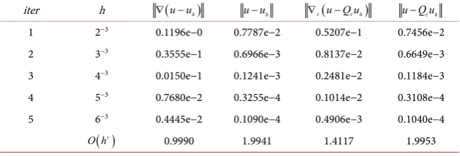
From Table 1, we observe that applying L2_{-projections to the existing}

numer-ical solution reduced the errors in L2 _{norm and in H}

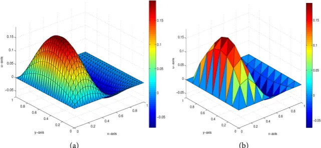
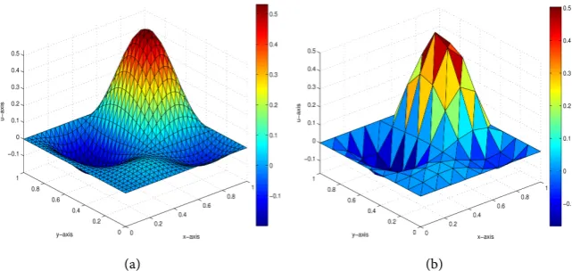
1 norm. Surface plots of

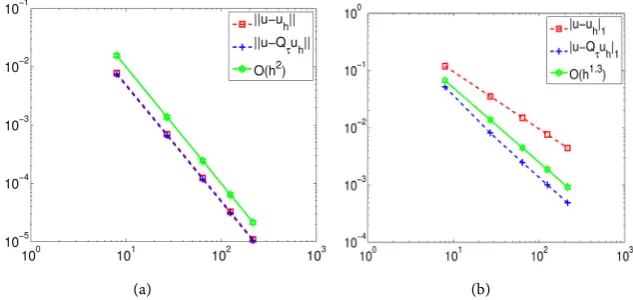
nu-merical solutions, uh in fine meshes and Q uτ h in coarse meshes, are shown in Figure 1. In L2 _{norm the error convergence rate of}

h

u Q u

−

τ and the error

convergence rate of

u u

−

h are similar to the theoretical convergence rate, which is shown as _{O h}

( )

2 _{(see Figure 2). However, in H}

1 norm the error

con-vergence rate of

u Q u

−

τ h₁ is higher than the optimal error convergence rate of

1

h

u u

−

_{and the error convergence rate of the numerical example, O h}

( )

1.42 _,

Table 1. Numerical error approximation results using CFEM in Example 1,

(

) ( )

cos 0.5π sin π

u y= y x .

iter h ∇(u u− h) u u− h ∇τ(u Q u− τ h) u Q u− τ h

1 2−3 _{0.1196e−0 0.7787e−2 0.5207e−1 0.7456e−2}

2 3−3 _{0.3555e−1 0.6966e−3 0.8137e−2 0.6649e−3}

3 4−3 _{0.0150e−1 0.1241e−3 0.2481e−2 0.1184e−3}

4 5−3 _{0.7680e−2 0.3255e−4 0.1014e−2 0.3108e−4}

5 6−3 _{0.4445e−2 0.1090e−4 0.4906e−3 0.1040e−4}

( )

r

[image:5.595.209.539.609.721.2]

DOI: 10.4236/am.2018.96047 696 Applied Mathematics

(a) (b)

Figure 1. Surface plots of approximation solution using CFEM in Example 1,

(

)

cos 0.5π sin(π )

u y= y x _{. (L): Surface plot of} u_h. (R): Surface of plot of Q uτ h.

[image:6.595.213.535.67.221.2]

(a) (b)

Figure 2. Error convergence rates using CFEM in Example 1,

(

)

cos 0.5π sin(π )

u y= y x . (L): _L2 _{norm error. (R):} 1

H norm error.

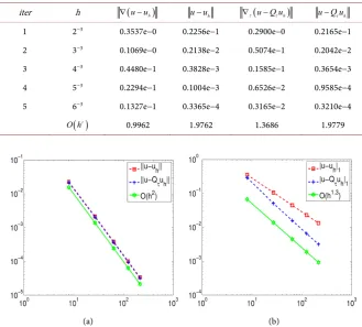
exceeds its theoretical error convergence rate, which is shown as _{O h}

( )

1.33 _{. As}

we expect from the theoretical results (11) and (12), the numerical example shows some superconvergence in H1 norm but not in L2 norm. The numerical

Example 1 supports the theoretical results in [16] and confirms the supercon-vergence of CFEM for second-order elliptic problems.

Example 2 Let the domain

Ω =

[ ] [ ]

0,1 0,1

×

_{and the analytical solution to the}

problem is given as

(

1

) (

1 .

)

u x

=

−

x y y

−

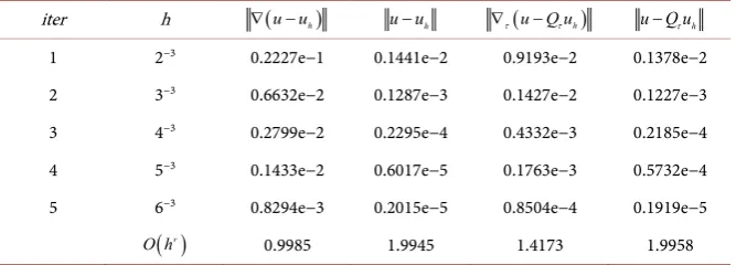
From Table 2, we confirm that the numerical Example 2 supports the theo-retical results in [16]. In L2 _{norm the error convergence rate of}

h

u Q u

−

τ is

similar to the error convergence rate of

u u

−

h which is about the same as the theoretical result in (11), which is shown as _{O h}

( )

2 _{in Figure 3. The error}

convergence rate of

u Q u

−

τ h₁ is about O h

( )

1.42 and the error convergence rate of

u u

−

h₁ is about

O h

( )

. In H1 norm the exact solution u clearly has

[image:6.595.216.533.274.424.2]

DOI: 10.4236/am.2018.96047 697 Applied Mathematics

[image:7.595.217.535.68.219.2]

(a) (b)

Figure 3. Error convergence rates using CFEM in Example 2, u x= 1

(

−x y y

) (

−1

)

. (L):

2

L norm error. (R): H1 norm error.

(a) (b)

Figure 4. Surface plots of approximation solution using CFEM in Example 2,

(

) (

)

= 1 1

u x −x y y− . (L): Surface plot of uh. (R): Surface plot of Q uτ h.

Table 2. Numerical error approximation results using CFEM in Example 2,

(

1

)

cos 1.5π

(

)

u x= −x y y .

iter h ∇(u u− h) u u− h ∇τ(u Q u− τ h) u Q u− τ h

1 2−3 _{0.2227e−1 0.1441e−2 0.9193e−2 0.1378e−2}

2 3−3 _{0.6632e−2 0.1287e−3 0.1427e−2 0.1227e−3}

3 4−3 _{0.2799e−2 0.2295e−4 0.4332e−3 0.2185e−4}

4 5−3 _{0.1433e−2 0.6017e−5 0.1763e−3 0.5732e−4}

5 6−3 _{0.8294e−3 0.2015e−5 0.8504e−4 0.1919e−5}

( )

r

O h _{0.9985 1.9945 1.4173 1.9958}

also supports the theoretical results in [16] and confirms the superconvergence of CFEM for second-order elliptic problems.

Example 3 Let the domain

Ω =

[ ] [ ]

0,1 0,1

×

_{and the analytical solution to the}

problem is given as

(

1

)(

1

) ( )

sin 2

π

.

[image:7.595.217.537.277.425.2] [image:7.595.207.541.507.627.2]

DOI: 10.4236/am.2018.96047 698 Applied Mathematics From Table 3, the numerical approximation results show that after the post-processing all the errors are reduced. The exact solution in L2 _{norm of}

h

u Q u

−

τ has the similar error convergence rate as

u u

−

h , which shown as

( )

2

O h . In L2 _{norm, there is no improvement with the post-processing}

tech-nique. See Figure 5, in H1 norm L2-projection method improved the

conver-gence rate, which is shown as _{O h}

( )

1.3 _for

(

)

h u Q u

τ τ

∇ − _{. Figure 6 shows}

surface plots of Q uτ h and uh. The numerical Example 3 confirms the theoret-ical results in [16].

Example 4 Let the domain

Ω =

[ ] [ ]

0,1 0,1

×

and the exact solution is as-sumed to be

( )

(

)

sin 2

π

cos 1.5

π

.

u x

=

x y

y

From Table 4, we confirm that the numerical Example 4 supports the theo-retical results in [16]. In L2 _{norm the error convergence rate of}

h

u Q u

−

τ is

similar to the error convergence rate of

u u

−

h which is about the same as the theoretical result, O h

( )

2 . However, in H1 norm the exact solution u has some

[image:8.595.212.535.324.486.2]

(a) (b)

Figure 5. Error convergence rates using CFEM in Example 3,

(

)(

) (

)

= 1 1 sin 2π

u y −y −x x . (L): _L2 _{norm error. (R):} 1

H norm error.

(a) (b)

Figure 6. Surface plots of approximation solution using CFEM in Example 3,

(

)(

) (

)

= 1 1 sin 2π

[image:8.595.213.534.537.685.2]

DOI: 10.4236/am.2018.96047 699 Applied Mathematics superconvergence. The error convergence rate of

u Q u

−

τ h₁ is about 34% faster than the error convergence rate of

u u

−

h₁ and meets the theoretical minimum error convergence rate, _{O h}

( )

1.33 _{. See Figure 7, in}

L2 _{norm there is no difference}

in error convergence rates but in H1 norm applying L2-projection methods to the

[image:9.595.206.540.224.343.2]

existing numerical approximations improved the errors and produced some su-perconvergence. Figure 8 shows surface plots of the numerical approximations of (2) before and after the post-processing.

Table 3. Numerical error approximation results using CFEM in Example 3,

(

1

)(

1

) (

sin 2π

)

u y= −y −x x .

iter h ∇(u u− h) u u− h ∇τ(u Q u− τ h) u Q u− τ h

1 2−3 _{0.1162e−0 0.7440e−2 0.8059e−1 0.7070e−2}

2 3−3 _{0.3444e−1 0.6787e−3 0.1389e−1 0.6415e−3}

3 4−3 _{0.1452e−1 0.1211e−3 0.4342e−2 0.1144e−3}

4 5−3 _{0.7439e−2 0.3178e−4 0.1787e−2 0.3000e−4}

5 6−3 _{0.4305e−2 0.1064e−4 0.8670e−3 0.1005e−4}

( )

r

[image:9.595.207.537.389.686.2]

O h _{0.9999 1.9880 1.3726 1.9899}

Table 4. Numerical error approximation results using CFEM in Example 4,

(

)

(

)

sin 2π cos 1.5π

u x= x y y _.

iter h ∇(u u− h) u u− h ∇τ(u Q u− τ h) u Q u− τ h

1 2−3 _{0.3537e−0 0.2256e−1 0.2900e−0 0.2165e−1}

2 3−3 _{0.1069e−0 0.2138e−2 0.5074e−1 0.2042e−2}

3 4−3 _{0.4480e−1 0.3828e−3 0.1585e−1 0.3654e−3}

4 5−3 _{0.2294e−1 0.1004e−3 0.6526e−2 0.9585e−4}

5 6−3 _{0.1327e−1 0.3365e−4 0.3165e−2 0.3210e−4}

( )

r

O h 0.9962 1.9762 1.3686 1.9779

(a) (b)

Figure 7. Error convergence rates using CFEM in Example 4,

(

)

(

)

sin 2π cos 1.5π

u x= x y y . (L): _L2 _{norm error. (R):} 1

DOI: 10.4236/am.2018.96047 700 Applied Mathematics

[image:10.595.213.534.73.225.2]

(a) (b)

Figure 8. Surface plots of approximation using CFEM in Example 4,

(

)

(

)

sin 2π cos 1.5π

u x= x y y . (L): Surface plot of uh. (R): Surface plot of Q uτ h.

With numerical experiments we support the theoretical results in [16] and confirm the superconvergence of CFEM for second-order elliptic problems.

5. Conclusion

The L2_{-projection to the existing numerical approximation} h

u produced some superconvergence in H1 norm, convergence rate ≥1.3, but did not affect the

convergence rate in L2 _{norm. With the numerical experiments we can}

conclu-sively support the theoretical result and confirm the superconvergence of CFEM for second-order elliptic problems by L2_{-projection method.}

Acknowledgements

We thank the Editor and the peer-reviewers for their comments. Research of Anna Harris is funded by the National Science Foundation Historical Black Col-leges and Universities Undergraduate Program Research Initiative Award grant (#1505119). This support is greatly appreciated.

References

[1] Bramble, J.H. and Schatz, A.H. (1977) Higher Order Local Accuracy by Averaging in the Finite Element Method. Mathematics of Computation,31, 94-111.

https://doi.org/10.1090/S0025-5718-1977-0431744-9

[2] Douglas Jr., J. and Wang, J. (1989) A Superconvergence for Mixed Finite Element Methods on Rectangular Domains. Calcolo, 26, 121-134.

https://doi.org/10.1007/BF02575724

[3] Ewing, R.E., Lazarov, R. and Wang, J. (1991) Superconvergence of the Velocity along the Gauss Lines in Mixed Finite Element Methods. SIAM Journal on Numer-ical Analysis, 28, 1015-1029. https://doi.org/10.1137/0728054

[4] Krizek, M. and Neittaanmaki, P. (1984) Superconvergence Phenomenon in the Fi-nite Element Method Arising from Averaging Gradient. Numerische Mathematik, 45, 105-116. https://doi.org/10.1007/BF01379664

Varia-DOI: 10.4236/am.2018.96047 701 Applied Mathematics

tional-Difference Methods in Mathematical Physics, Part II, Moscow, 13-25. [6] Lin, Q. (1992) Global Error Expansion and Superconvergence for Higher Order

In-terpolation of Finite Element. Journal of Computational Mathematics, 10, 286-289. [7] Oganesyan, I.A. and Rukhovetz, L.A. (1969) Study of the Rate of Convergence of

Variational Difference Scheme for Second-Order Elliptic Equations in Two-Dimensional Field with a Smooth Boundary. USSR Computational Mathematics and Mathemat-ical Physics,9, 158-183. https://doi.org/10.1016/0041-5553(69)90159-1

[8] Wahlbin, L.B. (1995) Superconvergence in Galerkin Finite Element Methods. Springer, New York. https://doi.org/10.1007/BFb0096835

[9] Zlamal, M. (1978) Superconvergence and Reduced Integration in the Finite Element Method. Mathematics of Computation, 32, 663-685.

https://doi.org/10.2307/2006479

[10] Schatz, A.H., Sloan, I.H. and Wahlbin, L.B. (1996) Superconvergence in Finite Ele-ment Methods and Meshes That Are Symmetric with Respect to a Point. SIAM Journal on Numerical Analysis, 33, 505-521. https://doi.org/10.1137/0733027

[11] Douglas, J., Dupont, T. and Wheeler, M.F. (1974) An l∞ _{Estimate and a}

Super-convergence Result for a Galerkin Method for Elliptic Equations Based on Tensor Products of Piecewise Polynomials. RAIRO: Analyse Numérique, 8, 61-66.

[12] Douglas, J. and Dupont, T. (1973) Some Superconvergence Results for Galerkin Methods for the Approximation Solution of Two-Point Boundary Value Problems.

Topics in Numerical Analysis, 89-92.

[13] Wang, J. (1991) Superconvergence and Extrapolation for Mixed Finite Element Methods on Rectangular Domains. Mathematics of Computation, 56, 477-503.

https://doi.org/10.1090/S0025-5718-1991-1068807-0

[14] Zienkiewicz, O.C. and Zhu, J.Z. (1992) The Superconvergent Patch Recovery and a Posteriori Error Estimates. Parts 1: The Recovery Technique. International Journal for Numerical Methods in Engineering, 33, 1331-1364.

https://doi.org/10.1002/nme.1620330702

[15] Zienkiewicz, O.C. and Zhu, J.Z. (1992) The Superconvergent Patch Recovery and a Posteriori Error Estimates. Parts 2: Error Estimates and Adaptivity. International Journal for Numerical Methods in Engineering, 33, 1365-1382.

https://doi.org/10.1002/nme.1620330703

[16] Wang, J. (2000) A Superconvergence Analysis for Finite Element Solutions by the Least-Square Surface Fitting on Irregular Meshes for Smooth Problems. Journalof MathematicalStudy, 33, 229-243.