© 2019, IRJET | Impact Factor value: 7.211 | ISO 9001:2008 Certified Journal | Page 2760
“RAINFALL SIMULATION USING ANN BASED GENEREALIZED FEED
FORWARD AND MLR TECHNIQUE”
Karuna Singh
1, Dr. Vikram Singh
2, Dr. S.K. Srivastava
3, Er. C.J Wesley
41
PG Scholar SHUATS Allahabad U.P
2,4
Assistant Professor SHUATS Allahabad U.P
3
Associate Professor SHUATS Allahabad U.P
---***---Abstract -Rainfall modeling is one of the most importanttopics in water resources planning, development and management on sustainable basis. In this study an effort has been carried out for the development of Generalized Feed Forward (GFF) and Multi Linear Regression (MLR) technique for daily monsoon rainfall prediction of Satna (M.P.). The daily data of monsoon period from (1st June to 30th September) of year 2004-2011 were used for training of models and data of remaining years 2012-2013were used for testing of the models. The NeuroSolution 5.0 software and Microsoft Excel were used in analysis and the performance evaluation indices for developed models, respectively. The best input combination was identified using the input-output combination for the simulation. On the basis input combination, 10 best combinations. The input pairs in the training data set were applied to the network of a selected architecture and training was performed.
Key Words: (Rainfall Simulation, Ann Based GFF Techniques, MLR Techniques, Validation)
1. INTRODUCTION
Rainfall prediction is one of the most important and challenging tasks in the modern world. In general, climate and rainfall are highly non-linear and complicated phenomena, which require advanced computer modeling and simulation for their accurate prediction. An Artificial Neural Network (ANN) can be used to predict the behavior of such nonlinear systems. ANN has been successfully used by most of the researchers in this field for the last twenty-five years survey of the available literature of some methodologies employed by different researchers to utilize ANN for rainfall prediction. The survey also reports that rainfall prediction using ANN technique is more suitable than traditional statistical and numerical methods, there are two main approaches in rainfall forecasting, numerical and statistical methods. The performance of the numerical method depends on the initial condition, which is inherently incomplete. The method is poor for long-range prediction. On the other hand, the statistical method is widely used for long-term rainfall prediction. In their studies stated those statistical method performances were successful in normal monsoon rainfall but fail in extreme monsoon years. In addition, the statistical method is useless for highly nonlinear relationship between rainfall and its predictors and there is no ultimate end in finding the best predictors.
2. REVIEW AND LITERATURE
ElShafie et al. (2011) have developed two rainfall prediction models i.e. Artificial Neural Network model (ANN) and Multi Regression model (MLR) and implemented in Alexandria, Egypt. They have used statistical parameters such as the Root Mean Square Error, Mean Absolute Error, Coefficient Of Correlation and BIAS to make the comparison between the two models and found that the ANN model shows better performance than the MLR model.1.2 Sub Heading 2
Saha et al. (2012) develop suitable Regression and Artificial Neural Network (ANN) models using identified 144 randomly selected indicators data sets over nine years historical time periods, collected from a successful case study namely “Semi micro watershed, Sehore District, Madhya Pradesh, India”. Regression and ANN decision support system prediction models have been developed with eight most dominating parameters which have found most significant effect on livelihood security. The comparison study of these two models have indicated that, the statistical yield predicted through ANN models performed better than that predicted through regression models. The study has recommended the use of such models for improvement of similar degraded watershed for future reference.
Chua et al. (2013) have employed several soft computing approaches for rainfall prediction. They have considered two aspects to improve the accuracy of rainfall prediction: (1) carrying out a data-preprocessing procedure and (2) adopting a modular modeling method. The proposed preprocessing techniques included moving average (MA) and singular spectrum analysis (SSA). The modular models were composed of local support vector regression (SVR) models or/and local artificial neural network (ANN) models. The ANN was used to choose data- preprocessing method from MA and SSA. Finally, they have showed that the MA was superior to the SSA when they were coupled with the ANN.
© 2019, IRJET | Impact Factor value: 7.211 | ISO 9001:2008 Certified Journal | Page 2761
monthly rainfall time series at the Ca Mau hydrological station in Vietnam were decomposed by using the two pre-processing data methods applied to five sub-signals at four levels by wavelet analysis, and three sub-sets by seasonal decomposition. After that, the processed data were used to feed the feed-forward Neural Network (ANN) and Seasonal Artificial Neural Network (SANN) rainfall prediction models.
3. MATERIALS AND METHOD
3.1 Location of study area:
The study area located between 24°56'09.31"N, 25°10'53.19N latitude and 80°44'23.31"E, 80°52'44.53"E longitude (approx.) with an average elevation of 315 meters (1,352 feet).
3.2 Climatic Characteristics
The climate of Satna district is characterized by a hot summer with general dryness, except during the south-west monsoon season. The normal annual rainfall of Satna district is 1092.1 mm. The district receives maximum rainfall during south-west monsoon period (i.e. June to September) and about 87.7% of annual rainfall is received during this period. Only 12.3% of the annual rainfall takes place between periods October to May.
3.3 Data Collection
The weather data (rainfall, minimum and maximum temperature, relative humidity) of monsoon season (1st June to 30th September) during the years 2004-2013 were obtained from global weather data for SWAT website.
3.4 Methodology
[image:2.595.39.283.286.382.2]In this study, the soft computing techniques such as Generalized Feed Forward (GFF) based ANN and statistical multiple linear regression (MLR) have been developed for simulating the rainfall in Satna district. The methodology of developing the GFF and MLR models along with training and testing of the developed models, the NeuroSolution 5.0 software and Microsoft Excel were used in analysis and the performance evaluation indices for developed models.
Figure 3.1 Basic structure of ANN
3.4.1 Generalized Feed Forward (GFF)
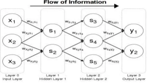
[image:2.595.310.560.389.531.2]In this study, a different approach was used to obtain the network architecture. Instead of limiting the size of the networks, complex networks were developed with a high number of connections. The objective was to obtain a network with greater capacity for establishing generalized relationships between the parameters on which rainfall depends.
Fig 3.2 Four layer feed forward neural network
3.4.2 Multiple Linear Regression (MLR)
Multiple Linear Regression (MLR) is simply extended form of Simple regression in which two or more variables are independent variables are used and can be expressed as (Kumar and Malik, 2015):
Where,
Y = Dependent variable;
α = Constant or intercept;
© 2019, IRJET | Impact Factor value: 7.211 | ISO 9001:2008 Certified Journal | Page 2762
X1 =First independent variable that is explaining the variance in Y;
β2 = Slope (Beta coefficient) for X2;
X2 = Second independent variable that is explaining the variance in Y;
p= Number of independent variables;
βp= Slope coefficient for Xp;
Xp= pth independent variable explaining the variance in Y.
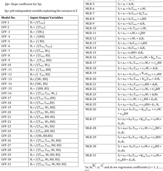
Model No. Input-Output Variables
GFF-1 Rt = f (Tmax)
GFF-2 Rt = f (Tmin)
GFF -3 Rt = f (WS)
GFF -4 Rt = f (RH)
GFF -5 Rt = f ( RS)
GFF -6 Rt = f (Tmax Tmin,)
GFF -7 Rt = f (Tmax, WS)
GFF -8 Rt = f (Tmax, RS)
GFF -9 Rt = f (Tmax, RH)
GFF-10 Rt = f (Tmin, WS)
GFF -11 Rt = f (Tmin, RH)
GFF -12 Rt = f ( Tmin, RS)
GFF -13 Rt= f (WS, RH)
GFF -14 Rt= f (WS, RS)
GFF -15 Rt = f (RH, RS)
GFF-16 Rt = f (Tmax Tmin, WS, )
GFF-17 Rt = f (Tmax Tmin,,RH)
GFF-18 Rt = f (Tmax Tmin,RS)
GFF-19 Rt = f (Tmax, WS, RH)
GFF-20 Rt = f (Tmax, WS, RS)
GFF-21 Rt = f (Tmax, RH, RS)
GFF-22 Rt = f (Tmin, WS, RH)
GFF-23 Rt = f (Tmin, WS, RS)
GFF-24 Rt = f (Tmin,,RH, RS)
GFF-25 Rt = f (WS, RH,RS)
GFF-26 Rt = f (Tmax Tmin, WS, RH)
GFF-27 Rt = f (Tmax ,Tmin,, RH, RS)
GFF-28 Rt = f (Tmax Tmin, WS, RS)
GFF-29 Rt = f (Tmax, WS, RH, RS)
GFF-30 Rt = f (Tmin,, WS, RH, RS)
GFF-31 Rt = f (Tmax ,Tmin, WS, RH, RS)
Table -3.1: Input-output combinations for GFF models for rainfall simulation
Model No. Input-Output Variables*
MLR-1 St = a1 + b1Tmax
MLR-2 St = a2 + c1Ws
MLR-3 St = a3 + b2Tmin
MLR-4 St = a4 + c2RH
MLR-5 St = a5 + d1Rs
MLR-6 St = a6 + b3Tmax + c3Ws
MLR-7 St = a7 + b4Tmax+ Tmin
MLR-8 St = a8 + b5Tmax + c4RH
MLR-9 St = a9 + b6Tmax + d2Rs
MLR-10 St = a10 + b7 Tmin+ c5Ws
MLR-11 St = a11 + c6Ws+ RH
MLR-12 St = a12 + c7Ws + d3Rs
MLR-13 St = a13 + b8Tmin + c8RH
MLR-14 St = a14 +b9Tmin + d4Rs
MLR-15 St = a15 +c9RH+ d5Rs
MLR-16 St = a16 + b10Tmax+c10Ws + Tmin
MLR-17 St = a17 + b11Tmax + c11Ws+ + RH
MLR-18 St = a18 + b12Tmax + c12Ws + d6Rs
MLR-19 St = a19 + b13Tmax + Tmin + c13RH
MLR-20 St = a20 + b14Tmax + Tmin + d7Rs
MLR-21 St = a21 + b15Tmax+ c14RH + d8Rs
MLR-22 St = a22 + b16Tmin + c15Ws + RH
MLR-23 St = a23 + b17Tmin + c16Ws + d9Rs
MLR-24 St = a24 + c17Ws + RH+ d10Rs
MLR-25 St = a25 + b18Tmin + c18RH+ d11 Rs
MLR-26 St = a26+ b19Tmax + Tmin + c19Ws
+ RH
MLR-27 St = a27+ b20Tmax + Tmin + c20Ws+
d12Rs
MLR-28 St = a28+ b21Tmax + c21Ws + RH+
d13Rs
MLR-29 St = a29+ b22Tmax + Tmin + c22RH+
d14Rs
MLR-30 St = a30+ b23Tmin+ c23Ws+ RH+
d15Rs
MLR-31 St = a31+ b24Tmax + min + c24Ws+
RH+ d16Rs
[image:3.595.36.561.197.748.2]© 2019, IRJET | Impact Factor value: 7.211 | ISO 9001:2008 Certified Journal | Page 2763
Table 3.2 Input-output combinations MLR models forrainfall simulation at Satna (M.P.)
4. RESULTS AND DISCUSSION
The performance of the development model were evaluated qualitatively and quantitatively by the visual observation, and based on various statistical and hydrological indices such as correlation coefficient (r), coefficient of efficiency (CE) and mean squared error (MSE). The thirty one model having high values of rand CE and lower values of MSE is considered as the better fit model.
4.1 Rainfall Modeling using GFF
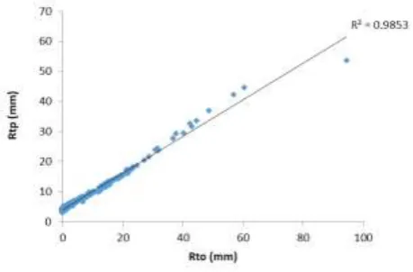
[image:4.595.330.558.50.245.2]The increased values of CE and r by GFF models during testing period indicate good generalization capability of the selected GFF models. It is clear from table 4.1 GFF-2 model with 1-2-1 architecture (one inputs; four hidden neurons; one output) had lower MSE (0.00140) and higher CE (0.8336) and r (0.9926) values in the testing phase.
Table 4.1 Statistical indices for GFF models for rainfall simulation during testing
S.N
O MODEL STRUCTURE TESTING
MSE r R2 CE
1 M1 (1-2-1) 0.001
40 0.9926 0.9853 0.8336
2 M2 (1-2-1) 0.001
43 0.9944 0.9889 0.8297
3 M1 (1-4-1) 0.001
49 0.9892 0.9786 0.8226
4 M9 (2-8-1) 0.001
53 0.9736 0.9479 0.8179
5 M8 (2-6-1) 0.001
681 0.9761 0.9529 0.8006
6 M15 (2-8-1) 0.001
701 0.9612 0.9239 0.7981
7 M2 (2-8-1) 0.001
73 0.9950 0.9902 0.7939
8 M13 (2-10-1) 0.001
78 0.9632 0.9279 0.7882
9 M13 (2-8-1) 0.001
81 0.9589 0.9197 0.7842
10 M4 (1-2-1) 0.001
[image:4.595.314.544.291.442.2]843 0.96984 0.9406 0.7813
[image:4.595.31.292.377.698.2]Fig 4.1 Comparison of observed and predicted rainfall by model 1, Neuron 2, during the validation period
Fig 4.2 Correlation between observed and predicted rainfall by model 1, Neuron 2 during the validation period.
4.2 Rainfall Modeling using MLR
On the basis of the lowest value of MSE and the highest values of r and CE, the MLR-31 model was found to be the best performing model. Therefore, according to MLR-31 model, the current day’s rainfall depends on minimum temperature, relative humidity and rainfall of current day.
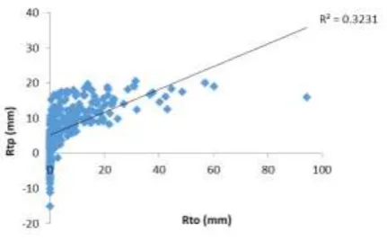
The MSE varied from 96.8136 to 105.2627 m3/s; the CE varied from 0.3231 to 0.2640; and r varied from 0.5684 to 0.5138.
Table 4.2 Statistical indices for selected MLR rainfall models during testing period (2012-2013)
Model No.
Statistical index
MSE CE r R2
M31 96.8136 0.3231 0.5684 0.3231
M30 96.9728 0.3219 0.5674 0.3219
M27 96.9379 0.3222 0.5258 0.322
[image:4.595.40.532.379.798.2]© 2019, IRJET | Impact Factor value: 7.211 | ISO 9001:2008 Certified Journal | Page 2764
M17 100.49 0.2977 0.5456 0.2977
M21 100.457 0.2976 0.5455 0.2976
M9 101.017 0.2937 0.5419 0.2937
M28 101.172 0.2765 0.525 0.2765
M15 102.705 0.2819 0.5309 0.2819
M6 105.26 0.2640 0.5138 0.2640
[image:5.595.47.263.289.406.2]The observed (Rto) and predicted (Rtp) rainfall simulated by MLR models were compared in the form of graph and scatter-plot as shown in Figs. 4.11 to 4.20. The rainfall graphs indicate that the models under predict the peak rainfall as confirmed by the scatter plots also. This study gave clear indication of non-applicability of the MLR model to simulate rainfall for the study area due to low values of CE and r.
Fig 4.3 Comparison of observed and predicted rainfall by MLR-31, during the validation period.
Fig 4.22 Correlation between observed and predicted rainfall by MLR-31, during the validation period.
3. CONCLUSIONS
1. Rainfall can be simulated by using GFF model with input parameters as maximum temperature, minimum temperature, relative humidity and rainfall.
2. The predicted values of rainfall using GFF (Generalized Feed Forward) were found to be much closer to the observed value of rainfall as compared to MLR.
3. On the basis of lower MSE value and higher CE and r values, GFF-1 model was found to be the best model.
4. It was clearly evident that MLR model fits very poorly for the dataset under study.
REFERENCES
[1] C. L. Wu, K. W Chau, and C. Fan, 2013, “Prediction of Rainfall Time Series Using Modular Artificial Neural
Networks Coupled with Data Preprocessing
Techniques”, Journal of Hydrology, Vol. 389, No. 1-2, pp. 146-167.
[2] Duong Tran Anh 1,3,* , Thanh Duc Dang 2,3 and Song Pham Van 3 (2019) Improved Rainfall Prediction Using Combined Pre-Processing Methods and Feed-Forward Neural Networks.
[3] El-shafie, M. Mukhlisin, A. Najah Ali and M. R. Taha,
2011, “Performance of artificial neural network and regression techniques for rainfall-runoff prediction”, International Journal of the Physical Sciences, Vol. 6(8), pp. 1997-2003.
[4] Saha, N., Jha, A. K., Pathak, K. K. 2012 “Comparison of Regression and Artificial Neural Network Impact Assessment Models: A Case Study of Micro-Watershed Management in India”
BIOGRAPHIES
1PG Scholar SHUATS Allahabad U.P
2Assistant Professor SHUATS
Allahabad U.P
3Associate Professor SHUATS Allahabad U.P
4Assistant Professor SHUATS
[image:5.595.43.259.457.591.2]