Complex Valued Recurrent Neural Network: From
Architecture to Training
Alexey Minin1,2, Alois Knoll1, Hans-Georg Zimmermann2
1Technische Universität München—Robotics and Embedded Systems, München, Germany; 2Siemens AG, Corporate Technology, München, Germany.
Email: [email protected]
Received December 7th,2011; revised February 11th, 2012; accepted March 18th, 2012
ABSTRACT
Recurrent Neural Networks were invented a long time ago, and dozens of different architectures have been published. In this paper we generalize recurrent architectures to a state space model, and we also generalize the numbers the net- work can process to the complex domain. We show how to train the recurrent network in the complex valued case, and we present the theorems and procedures to make the training stable. We also show that the complex valued recurrent neural network is a generalization of the real valued counterpart and that it has specific advantages over the latter. We conclude the paper with a discussion of possible applications and scenarios for using these networks.
Keywords: Complex Valued Neural Networks; Complex Valued System Identification; Recurrent Neural Networks; Complex Valued Recurrent Neural Networks
1. Introduction
Current paper aims to give the complete guidance from the state space models with complex parameters to the complex valued recurrent neural network of a special type. This paper is unique in translating the models sug- gested by Zimmermann in [1] to the complex valued case. Moreover one can see unique approach for managing the problems with transition functions which arise in com- plex-valued case, new approach for treating the error function which gives the unique advantages for the com- plex-valued neural networks. A lot of research in the area of complex valued recurrent neural networks is currently ongoing. One can find the works of Mandic [2,3], Adali [4] and Dongpo [5]. Mandic and Adali pointed out the advantages of using the complex valued neural networks in many papers. This paper will supply the neural net- work community with new architecture which shows better results in its complex-valued case.
We start the paper with the description on the state space models and then proceed with the very detailed explanations regarding the complex valued neural net- works. We discuss complex valued system identification, error function properties in its complex valued case, complex valued back-propagation and break points with transition functions. Paper ends up with the small discus- sion on applications and advantages which arise form the complex valued case of the considered architecture.
State space techniques may be used to model recurrent
dynamical systems. There are two principle ways of modeling dynamical systems: 1) use a feed-forward neu- ral network and use delayed inputs or 2) use a recurrent architecture and model the dynamics itself. The first ap- proach is based on Takens theorem [6] that a dynamical system or the attractor of the dynamical system can be reconstructed by a set of previous values of the realiza- tions of the dynamical system (expectations). This is true for chaotic systems, but in real world applications feed forward networks cannot be used for forecasting the states of dynamical systems. Therefore, recurrent archi- tectures are the only sensible way of forecasting dyna- mical systems, i.e. to represent the dynamics in the
re-current connection weights. This approach was first sug- gested by Elman [7] and later extended by Zimmer- mann [8]. As an example for this paper we will consider the so called open-system for which we will build a state space model based on the recurrent complex valued neu- ral network. Such an open-system (open means that the system is driven not only by its internal state changes but also by external stimuli) is given as follows:
1 ,
t t
t t
t
s f s u
y g s
(1)
Here, the states of the system ( t1n) depend on the previous states as well as some system input t through some non-linear function f. The output of the system de-
pends on the current state of the system mapped through
S
another non-linear function g. A graphical representation
is in Figure 1.
In the rest of this paper, we will use networks described by Equation (1) and Figure 1. In order to generalize the approach, we now assume that the dynamic system’s behavior is described by complex numbers, which means that S u St, ,t t1,ytC and functions f g C, : C are
defined on the domain of complex numbers.
2. Complex Valued Neural Network
The Complex Valued Recurrent Neural Network (further CVRNN) is a straight forward generalization of the real- valued RNN. The algorithms which are used for CVR- NNs can be also used for RNNs without loss of general- ity. To describe the CVRNN we start with a feed-forward path, and then we will discuss the error back-propagation algorithm (further CVEBP) and the training of such ar- chitectures.
2.1. Architecture Description and Feed Forward Path
The system represented by Figure 1 and Equation (1) can be realized as follows (as suggested by Zimmermann [9]): consider a set of 3-layer-feed-forward networks (further FFNN), whose hidden layers are connected to each other. This connection represents the evolution of the corresponding dynamical system inside the RNN. The structure of this type of network is shown in Figure 2.
The dynamical system develops based on 1) internal evolution of the system state governed by the matrix A and
the activation function. Matrices B, Cconvert the exter-
nal stimulus to the state (in the sense of data compression) and produce the output from the state (state decompres- sion). Therefore, one can write the following system of equations, which describe the system in Figure 2.
1 ,
t t t
t t
s f s u y g s
y
u
[image:2.595.129.203.545.611.2]s
Figure 1. Dynamical system representation.
3 t u
2
t
S
2 t y
2
t
u
1
t
S
1 t
y
1
t
u
t S t
y
t
u
1
t
S
1 t
y
A A A
B B B B
C C C C
Figure 2. Recurrent neural network.
1 tanh
t t
t t
t
s s u
y s
A B
C (2) where we have selected as an activation func-
tion
tanh ·
·f , which performs the non-linear transformation
of the state. Thus, all temporal relations of the dynamical system are represented in the matrix A (to be learned during training), the compression, and the decompression ability represented by the matrixes B, C respectively
(note that all elements of matrixes A B Cij, ij, ijC are
complex numbers).
One word about the weights matrices: the matrices between the layers are always the same (suggested as the “shared weights concept” in [8]). It is exactly this prop- erty that makes this network recurrent. Next, we will discuss the back propagation for the shared weights con- cept.
Summarizing, the RNN has actuation inputs utC s
; it has observable outputs ytC, it has states tC,
which evolve under the regime of the matrix A, and it has a non-linear activation function f
· .2.2. Error Back Propagation for the CVRNN The first variant of Complex Valued Error Back Propa- gation was described by Haykin in [7]. First, we have to define the error function. Since, in the complex valued case there are no “greater/less than” relations, the output of the error function must be a real number in order to make it possible to evaluate the training result and to guide it into the direction of an error reduction. The pro- cedure of the whole network training is as follows: find the network parameters, which are those weights that produce the minimum of the error function:
t,
ˆ
w t tE w f u w y min (3)
where w are weights, f is the activation function, u are the
complex valued inputs of the system, and are ob- servables.
ˆt
y
One class of functions, which produces real-valued output from complex arguments, is the following:
, t
ˆt
, t
ˆt
E w y w u y y w u y R (4)
where the over bar denotes complex value conjugate
a ib
a ib.This current error function is not analytic, i.e., the de-
rivative d dE w is not defined over the entire range of
input values. Therefore, back propagation cannot be ap- plied.
The requirement for the analyticity of any function E
is given by the Cauchy-Riemann conditions:
,
,
,
and
u a b v a b u a b v a b
a b b a
,
[image:2.595.105.239.643.723.2]where the function E is described with the following
equation:
,
E z u a b iv a b,
,
(6) where are some real differentiable functions of two real variables.
·, ·
u v
The requirement for the error function to produce real output means that v
· 0.
0
,
E z u a b i v a b
(7)
If we want , we have to take an error function similar to (4) since our error function
· 0v
,E z u a b ,
the optimality conditions are given by:
, 0 , 0u a b a u a b
b (8)
The function u
· makes a mapping of the followingtype: instead of C .In order to calculate
the derivative of the function one should use the so called Wirtinger derivative (discussed, e.g., in Brand- wood [10]): the Wirtinger derivative with respect to z and
2
R R R
·u
z can be calculated in the following way:
1
, 2
1 ,
2
E E E
i z a i
z a b
E E E
i z a
z a b
b ib (9)
For the real functions of complex variables E z 0
therefore the minimization of the error function can be done in both directions z or z.
Now we have the derivatives of the error function de- fined in the Wirtinger sense.
Note that this error function “minimizes” the complex number, which in the Euler notation (see Equation (10)) would mean, that it minimizes both amplitude and phase of the com ich is in our case
:
plex number, wh
y w u, t yt
2 2 ·arctgRe Im
a b b
i
i a
r
y y i y a b e re
(10)
This error function has very unique and desirable properties. Let us describe these properties more in detail. We rewrite (4) into Euler notation:
ˆ ˆ
2 2
2cos
ˆ ˆ i i
E r r rr e e
(11)
The discriminant of (11) is negative and only can be equal to zero that the equation has 1 root:
2 2 2 2
ˆ ˆ 2ˆ
ˆ 4 c
0 then
os 4 sin 0
D r r r
r r
We can also rewrite (4) in the following way:
2 2 2 2
2 2
ˆ ˆ
ˆ ˆ
ˆ ˆ ˆ
, 2 ˆ ˆ min 2 a a b b
E y y a b a b aa bb
b
a a b
(12)
One can see that error function (4) minimizes both real and imaginary parts of the complex number.
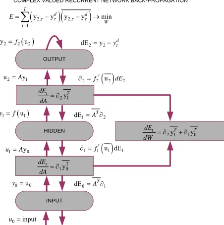
After defining a suitable error-function, we can now start with the CVEBP description. The procedure for CVEBP is shown in Figure 3. It follows the description in [9] or the RNN. The “ladder” algorithm allows a local and efficient computation of the recurrent network partial derivatives of the error with respect to the weights. The advantage of the algorithm shown in Figure 3 is that it intelligently unites the equations, the architecture and the locality of the CVEBP.
In Figure 3, one can see the CVEBP which is done for the shared matrix A and for the case when all NN pa- rameters are complex numbers.
2.3. Weights Update Rule for the CVRNN
In order to find the training rule for the weights update, we introduce the Taylor expansion of the error function:
12
T T
E w w E w g w w G w (13)
where (one can note that w has to be equal to the g
INPUT
T 1 0y
t
dE dA
0 u0
y dE0AT1
0 input
u
HIDDEN
1 y0
u A 1 f1
u dE1 1 1 u1
y f
1 2
dE T
A
1 2yT
t
dE dA 1 2
u Ay 2 f2
u2 dE2OUTPUT
2
2 2
y f u dE2 y2 d
y
COMPLEX VALUED RECURRENT NETWORK BACK-PROPAGATION
2,
2,
1
y y y y min
T
d d
W t
E
2y1 1 0y
t T T
dE
[image:3.595.310.536.478.705.2]dW
that Taylor expansion exist):
1
1 T :
d
t t
t
E y
y y
w T w
g
(14)
Following Johnson in his paper [11], two useful theo- rems to calculate the derivatives can be applied.
Theorem 1. If the function ( , )f z z is real-valued
and analytic with respect to or z z , all stationary
points can be found by setting the derivatives in Equation (9) with respect to either z or z to zero.
Theorem 2. By treating and z z as independent
variables, the quantity pointing in the direction of the maximum rate of change of f z z
, is z f z
.The proof of the theorems was demonstrated by John- son in [11].
Following Karla in [12] and Adali in [13], if minimi- zation goes in the direction of z, then
2
2 z
g g
. Otherwise, if we minimize in the di-
rection ofz , it results in g2Re
zg,zg
which need not necessarily be negative. This will lead us in the direction of a different minimization.
Following Theorem 2 and Equation (7), we consider 0
E w
. The Taylor expansion exists, since the deriva-
tives are defined and we can obtain a training rule for the optimization of weights in the direction of z :
w g
(15) Notice that Figure 3 is very similar to the real valued RNN, despite the conjugations instead of the transposes.
One should also note that this error function is univer- sal because it optimizes both the real and the imaginary part of the complex number. It has a simple derivative, and it is a parabola, which means it has only one mini- mum and smooth bounds. A typical convergence of the error during the training is presented in Figure 4.
Note that this error function is a real value. Figure 4 shows the modulus, i.e., exactly the error function, the
angle error is:
angle
Re Re
arctan arctan
Im Im
ˆ ˆ
E
y y
y y
(16)
After presenting the CVEBP and discussing the con- vergence of the error, we now discuss the final aspect of the CVRNN, which is the activation (or transition) func- tion.
2.4. Activation Function in the Complex Valued Domain
It is well known that for real valued networks, one of the requirements for the activation function is to be continu- ous (ideally: bounded), and it should have at least one derivative defined for the whole search space.
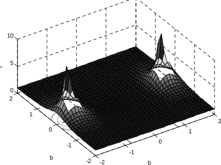
Unfortunately, this is not the case for the complex valued functions due to the Liouville theorem [10]. More- over, all transition functions which are not linear have an unlimited growth at their bounds (example: sine-function) or have singularity points an (example is the tanh-func- tion, see Figure 5 below).
Based on the following Theorem 3, we can make sev- eral remedies:
Liouville Theorem 3. If a complex analytic function is bounded and complex differentiable on the whole complex plain, it is constant.
This theorem has been proven in Remmert [14]. Remedy 1. Choose bounded functions which are only real valued but not complex differentiable:
tanh tanh
or i tanh i
f a ib a i b
f r e r e
(17)
[image:4.595.312.536.345.487.2]Remedy 2. Constrain the optimization procedure in order to stay in the area, where there are no singularities:
Figure 4. Error convergence for the absolute part of the error (dashed line) and for the phase of the error (solid line).
-2 -1
0 1
2
-2 -1 0 1 2 0 5 10
b b
f
[image:4.595.314.535.541.706.2]
logsig logsig ; 1
logsig logsig 1 logsig
i
z re z r
z z
z (18)
Remedy 3. All real analytic functions are differenti- able in complex domain using the Wirtinger Calculus.
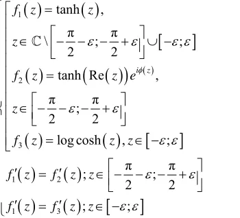
One can also try to substitute the problematic regions of the functions with different functions which do not have the problem in the following region (the problem is the presence of singularity point) following the (19) be- low:
1
2
3
1 2
1 3
tanh ,
π π
\ ; ;
2 2
tanh Re ,
π π
;
2 2
log cosh , ;
π π
; ;
2 2
; ;
i z
f z z
z
f z z e
z
f z z z
f z f z z
f z f z z
(19)
The result of such experiment is shown in Figure 6 below.
Typical use of the CVRNN with the activation func- tion tanh ·
will be possible with the non-linear func- tion, as long as the weights are initialized with small numbers and the error minimization goes in the correct direction (i.e., the error decreases and steps of the weightupdate becomes smaller as training time increases). Also, the weights do not go above 1, which means they do not approach the singularities of the function.
3. Summary and Outlook
[image:5.595.89.264.216.375.2]In this paper we discussed several aspects of CVRNN.
Figure 6. The transition function for the substitute functions.
We showed the architecture of the CVRNN, discussed the feed forward operation as well as the back-propag- ation CVEBP and the weights update rules. We discussed problems with the activation and error functions and showed how to overcome these problems.
There are many advantages of using CVRNN: continu- ous time modeling, modeling of electrical devices and energy grids, robust time series prediction, physical models of the brain, etc. Future work will focus on ap- plications and evaluation of CVRNNs.
REFERENCES
[1] H. G. Zimmermann and R. Neuneier, “Modeling Dynami- cal Systems by Recurrent Neural Networks, Data Mining II,” Second International Conference on Data Mining, Cambridge, 5-7 July 2000, pp. 557-566.
[2] S.-L. Gohand and D. Mandic, “A Complex-Valued RTRL Algorithm for Recurrent Neural Networks,” Neural Com- putation, Vol. 16, No. 12, 2006, pp. 2699-2713.
[3] P. Mandic, “Complex Valued Recurrent Neural Networks for Noncircular Complex Signals,” International Joint Con- ference on Neural Networks, 14-19 June 2009, pp. 1987-
1992.doi:10.1109/IJCNN.2009.5178960
[4] T. Adali and H. Li, “A Practical Formulation for Compu-tation of Complex Gradients and Its Application to Maximum Likelihood ICA,” 2007 IEEE International Conference on Acoustics, Speech and Signal Processing,
Vol. 2, 2007, pp. II-633-II-636. doi:10.1109/ICASSP.2007.366315
[5] D. P. Xu, H. S. Zhang and L. J. Liu, “Convergence Analysis of Three Classes of Split-Complex Gradient Al- gorithms for Complex-Valued Recurrent Neural Net- works,” Neural Computation, Vol. 22, No. 20, 2010, pp.
2655-2677.doi:10.1162/NECO_a_00021
[6] F. Takens, “Detecting Strange Attractors in Turbulence, Dynamical Systems and Turbulence,” Lecture Notes in Mathematics, Vol. 898, Springer-Verlag, New York, 1981,
pp. 366-381.
[7] H. Leung and S. Haykin, “The Complex Back Propaga- tion,” IEEE Transactions on Signal Processing, Vol. 39,
No. 9, 1991, pp. 2101-2104.doi:10.1109/78.134446 [8] G. Zimmermann, A. Minin and V. Kusherbaeva,
“Histori-cal Consistent Complex Valued Recurrent Neural Net- work,” Lecture Notes in Computer Science, Part 1, Vol. 6791, 2011, pp. 185-192.
doi:10.1007/978-3-642-21735-7_23
[9] H.-G. Zimmermann, A. Minin and V. Kusherbaeva, “Com- parison of the Complex Valued and Real Valued Neural Networks Trained with Gradient Descent and Random Search Algorithms,” 19th European Symposium on Arti- ficial Neural Networks, Bruges, 27-29 April 2011, pp.
216-222.
[10] D. H. Brandwood, “A Complex Gradient Operator and Its Application in Adaptive Array Theory,” IEEE Proceed- ings, F: Communications, Radar and Signal Processing,
[11] D. Johnson, “Optimization Theory,” Optimization Theory Page from the Connexions Project.
http://cnx.org/content/m11240/latest/
[12] P. Kalra, A. Gangal and D. Chauhan, “Performance Evalua- tion of Complex Valued Neural Networks Using Various Error Functions,” World Academy of Science, Engineer- ing and Technology, Vol. 29, 2007, pp. 27-32.
[13] H. L. Li and T. Adali, “A Class of Complex ICA Algo- rithms Based on the Kurtosis Cost Function,” IEEE Trans- actions on Neural Networks, Vol. 19, No. 3, 2008, pp.
408-420.doi:10.1109/TNN.2007.908636