RESEARCH ARTICLE
APPLICATION OF DATA MINING TECHNIQUES FOR OUTLIER MINING IN MEDICAL DATABASES
Dr. P. K. Srimani
1*and Manjula Sanjay Koti
21Former Chairman, Dept. of Computer Science and Maths, Bangalore University, Director, R&D, B.U., Bangalore 2Assistant Professor, Department of MCA, Dayananda Sagar College of Engineering, Bangalore
ARTICLE INFO ABSTRACT
Outlier detection has been a very important concept in the realm of data analysis and the complex relationships that appear with regard to patient symptoms, diagnoses and behavior are the most promising areas of outlier mining. This paper elaborates how the outliers can be detected by using statistical methods. The importance of outlier detection is due to the fact that outliers in data predict significant (and often critical) information in a wide variety of application domains. There are numerous different formulations of an outlier detection problem which have been explored in diverse disciplines such as statistics, machine learning, data mining and information theory. In fact, the study with medical data by using the DM techniques is virtually an unexplored frontier which needs extraordinary attention. In this study, the pima data set was used in the simulation carried out by TANAGRA. A total of 193 outliers were detected for the statistics namely leverage, R-standard, R-student, DFFITS, Cook’s D and covariance ratio. The results of the present investigation suggested that the extraordinary behavior of outliers facilitates the exploration of the valuable knowledge hidden in their domain and help the decision makers to provide improved, reliable and efficient healthcare services.
© Copy Right, IJCR, 2011, Academic Journals. All rights reserved
INTRODUCTION
Outlier detection is one of the most important tasks in data analysis. An outlier is an extreme observation. Typically points farther than, say, three or four standard deviations from the mean are considered as “outliers”. In regression however, the situation is somewhat more complex in the sense that some outlying points will have more influence on the regression than others. Outlier detection has been suggested for numerous applications, such as credit and fraud detection, clinical trials, voting, irregularity analysis, network intrusion, severe weather prediction, geographic information system, and other data mining tasks (Barnett and Lewis, 1995; Fawcett and Provost, 1997; Hawkins, 1980; and Penny and Jolliffe, 2001). Outliers in a data may be due to recording errors or system noise of various kinds, and as such needs to be cleaned with regard to extract, transform, clean and load phase (ETCL) of the data mining/KDD process. On the other hand an outlier or small group of outliers may be quite error-free recordings that represent the most important part of a data that deserve further careful inspection, e.g., an outlier might represent an unusually high response to a particular advertising campaign, or an unusually effective dose-response combination in a drug therapy (Ben-Gal I, 2005). Either way, it is quite important in data mining to detect outliers in large amounts of highly
*Corresponding author: [email protected],
multi-dimensional data. The multidimensional aspect of the data makes this task particularly challenging. This is because highly important and influential outliers can be completely hidden in one-dimensional views of the data, which renders ineffective one-dimensional outlier detection based on scanning one field (variable, attribute) at a time. There are three fundamental approaches to the problem of outlier detection:
Type 1 - Determines the outliers with no prior
knowledge of the data. This is essentially a learning approach analogous to unsupervised clustering. The approach processes the data as a static distribution, pinpoints the most remote points, and flags them as potential outliers.
Type 2 - Models both normality and abnormality.
This approach is analogous to supervised
classification and requires pre-labeled data, tagged as normal or abnormal.
Type 3 - Models only normality (or in a few cases
models abnormality). This is analogous to a semi-supervised recognition or detection task. It may be considered semi-supervised as the normal class is taught but the algorithm learns to recognize abnormality.
Outlier detection methods can be divided into univariate and multivariate methods.
ISSN:
0975-833X
International Journal of Current Research
Vol. 33, Issue, 6, pp.402-407, June, 2011
INTERNATIONAL JOURNAL OF CURRENT RESEARCH
Article History:
Received 14th
March, 2011 Received in revised form
19th
April, 2011
Accepted 21st
May, 2011
Published online 26nd
June 2011
Key words:
Outlier, Influential points, Statistical measures, Regression, Leverage, Cook’s distance,
Coefficient of determination R², Variance.
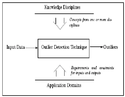
Fig 1. A general design of an outlier detection technique
The combination of data warehousing and data mining technology with evidence-based medicine as a new direction in modern health care introduces an innovative application field of information technology in healthcare industry(Kristin B. DeGruy,2000).As a result of this transformation, all parties are demanding greater and more detailed information on the effectiveness of the healthcare systems. More and more entities place data demands on other entities, and many healthcare organizations find themselves overwhelmed with data, but lack truly in valuable information (Varun Kumar, 2008).
MEDICAL AND PUBLIC HEALTH DATA
Outlier detection in the medical and public health domains typically work with patient records. The data can have outliers due to several reasons such as abnormal patient condition or instrumentation errors or recording errors. Thus the outlier detection is a very critical problem in this domain and requires high degree of accuracy. The data typically consists of records which may have several different types of features such as patient age, blood group and weight. The data might also have temporal as well as spatial aspect. Most of the current outlier detection schemes aim at detecting outlying records (Type I outliers). Typically the labeled data belongs to the healthy patients; hence most of the schemes adopt novelty detection approach (Kristin B. DeGruy, 2000).
DIABETES
Diabetes is an immune affecting disorder in which the body does not properly produce insulin. It is one of the most common chronic diseases, which can lead to serious long term complications. In diabetes there are two major types: Type I diabetes is caused by the failure of pancreas, in which case sufficient insulin will not be produced. Type I diabetes is usually diagnosed in children and young adults and was
previously known as Juvenile diabetes (Siti Farhanah et al.,
2005). In Type II diabetes, the body will be resistant to the insulin it makes, which leads to an uncontrolled increase of blood glucose unless the patient uses insulin or drug. The blood glucose level that is elevated for a long period can result in metabolic complications such as kidney failure, blindness, and an increased chance of heart attacks. To prevent or postpone such complications strict control over the diabetic
blood glucose level is needed. Numbers of computer-based systems are available to diagnose the disease. Type II diabetes is the most common form of diabetes. Diabetes mellitus is now a big growing health problem as it is the world’s fourth biggest cause of death particularly in the industrial and developing
countries (Rajeeb Dey et al., 2008). It is one of the most
common chronic diseases, which can lead to serious long-term complications and death.
LITERATURE SURVEY WITH REGARD TO PIMA INDIAN DIABETES DATA SET (PIDD)
Most of the work related to machine learning in the domain of diabetes diagnosis has concentrated on the study of the Pima Indian Diabetes data set in the UCI repository. This particular Pima data set has been widely used in machine learning experiments and is currently available through the UCI repository of standard data sets. This population has been studied continuously by the National Institute of Diabetes, Digestive and Kidney Diseases owing to the high incidence of diabetes. To study the positive as well as the negative aspects of the diabetes disease, Pima data set can be utilized, which contains 768 data samples. Each sample contains 8 attributes which are considered as high risk factors for the occurrence of diabetes, like
• Plasma glucose concentration • Diastolic blood pressure (mmHg) • Triceps skin fold thickness (mm) • 2-hour serum insulin (mu U/ms)
• Body mass index (weight in kg/(height in m)) 2 • Diabetes pedigrees function
• Age (years)
All the 768 examples were randomly separated into a training set of 576 cases (378, non-diabetic and 198, diabetic) and a test set of 192 cases (122 non-diabetic and 70 diabetic cases). In the above data set 268 patients are diabetic, which can be interpreted as “1” and the remaining patients are non-diabetic which can be interpreted as “0”. A brief description of the DM technique “Regression” is presented below:
REGRESSION
the model. Regression modeling has many applications in trend analysis, business planning, marketing, financial forecasting, time series prediction, biomedical and drug response modeling, and environmental modeling. To statisticians, unusual observations are generally either outliers or ‘influential’ data points. In regression analysis, the unusual observations are categorized as: outliers, high leverage points and influential observations. Outlier is an observation in a data set which appears to be inconsistent with the remainder of the
set of data(Johnson and Wichern, 2002). In other words, an
outlier is an observation that deviates so much from other observations as to create suspicion such that it was generated
by a different mechanism(Hawkins 1980).
Statistical outlier detection techniques are essentially model-based techniques; i.e. they assume or estimate a statistical model which captures the distribution of the data, and the data instances are evaluated with respect to how well they fit the model (V. Barnett and T. Lewis, 1994). If the probability of a data instance to be generated by this model is very low, the instance is deemed as an outlier. The need for outlier detection was experienced by statisticians as early as 19th century. The presence of outlying or discarding the observations in a data encouraged statistical analysis being performed on the data (Johnson, 2002). This led to the notion of accommodation or removal of outliers in different statistical techniques. Regression model based on outlier detection techniques typically analyze the residuals obtained from the model fitting process to determine how outlying is an instance with respect to the fitted regression model.
Grubbs' test is also called as ESD method (extreme studentized deviate). The first step is to quantify how far the outliers is from the others. Then the second step is to calculate the ratio Z as the difference between the outlier and the mean divided by the SD. If Z is large, the value is far from the others. Finally, the mean and SD are calculated from all values, including the outlier.
TREATMENT OF OUTLIERS
The key point to be stressed is that the above procedure can
only serve to identify points that are suspicious from a
statistical perspective. It does not mean that these points
should automatically be eliminated! The removal of data points can be dangerous. While this will always improve the “fit” of regression, and it may end up with destroying some of the most important information in data.
Methods to detect outliers
Eyeball Method – look at what falls away from the
line
Standardized or Studentized Residual Scores – look
at error scores such as those that are 2+ SD’s away from mean
Leveragibitiy Statistics (Hat Values) – difference of a
data point from the pooled mean.
Distance D as in Cook’s D – how much an
observation affects a change in a parameter estimate
(a or b weight). The correlation coefficient, r, is calculated using:
where,
is the variance of X.
is the variance of Y.
The covariance of x and y is given by,
Cook’s distance for points i & j is :
Where,
Di is the normalized measure of the influence of the point i on
all predicted mean values;
yi and yj are the regression estimates for the conditional mean at
the points
i and j, and s is the estimated root mean square error.
DFFITS
DFFITS is a diagnostic that shows how influential a point is in a statistical regression and is defined as the change ("DFFIT"), in the predicted value for a point, obtained when that point is left out of the regression, "Studentized" by dividing by the estimated standard deviation of the fit at that point:
where and are the predictions for the cases (i)with the
point i and (ii)without the point I; s(i) is the standard error
estimated without the point in question, and hii is the leverage
for the point.
EXPERIMENTAL RESULTS AND DISCUSSION:
Performance of a multiple linear regression analysis for a large set of data would be immensely time-consuming. Hence statistical analysis software could be used to quickly perform the test. The results obtained by using such a software clearly predicts: (i) R² value (ii) p-value. The results are presented in the figures 2 to 15.
Data set description
Workbook information
Number of sheets 1
Selected sheet diabeticdata
Sheet size 769 x 9
Data set size 769 x 9
Datasource processing
Computation time 156 ms
Fig 2. Workbook information Data set description 9 attribute(s), 768 example(s)
Attribute Category Information
PR Continue -
PG Continue -
DBP Continue -
TRICEPS Continue -
SERUM Continue -
BMI Continue -
PEDI Continue -
AGE Continue -
CLASS Continue -
Fig 3. Data set description Global results
Endogenous attribute CLASS
Examples 768
R² 0.303253
Adjusted-R² 0.295909
Sigma error 0.400210
F-Test (8,759) 41.2935 (0.000000)
Fig 4. Global results
The coefficient of determination R² is a valuable tool to evaluate the fit of a model. The regular R² always increases with the number of factors included in the model while the adjusted R² takes the complexity of the model into account. One reasonable criterion for a good model is to maximize the adjusted R². R² is a measure of how well future outcomes are
likely to be predicted by the model. Adjusted R2 is a
modification of R2 that adjusts for the number of explanatory
terms in a model. Unlike R2, the adjusted R2 increases only if
the new term improves the model beyond the expectation. The
adjusted R2 can be negative, and will always be less than or
equal to R2 .
An F-test is any statistical test in which the test statistic has the F-distribution under the null hypothesis. The F-test in one-way analysis of variance is used to assess whether the expected values of a quantitative variable within several pre-defined groups, differ from each other. The alpha value arising from a test gives the p-value. Degrees of freedom is an integer value measuring the extent to which an experimental design imposes constraints upon the pattern of the mean values of data from various meaningful subsets of data.
Analysis of variance
Source xSS d.f. xMS F p-value
Regression 52.9113 8 6.6139 41.2935 0.0000
Residual 121.5678 759 0.1602
Total 174.4792 767
Fig 5. Analysis of variance
If the p‐value is lower than the significance level of test α
(probability of the outcome under the null hypothesis), then the model is considered to be significant.
Coefficients
Attribute Coef. std t(759) p-value
Intercept -0.853894 0.085485 -9.988825 0.000000
PR 0.020592 0.005130 4.014026 0.000066
PG 0.005920 0.000515 11.492938 0.000000
DBP -0.002332 0.000812 -2.873049 0.004179
TRICEPS 0.000155 0.001112 0.138930 0.889542
SERUM -0.000181 0.000150 -1.205020 0.228571
BMI 0.013244 0.002088 6.343656 0.000000
PEDI 0.147237 0.045054 3.268030 0.001132
[image:4.612.313.553.277.552.2]AGE 0.002621 0.001549 1.692707 0.090922
Fig 6. Coefficients
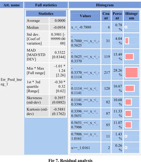
Residuals analysis
It is to be noted that residuals is the predicted value minus the actual value and it is the predicted error.
Att. name Full statistics Histogram
Err_Pred_lmr eg_1
Statistics
Average 0.0000
Median -0.0954
[image:4.612.313.553.278.550.2] [image:4.612.75.268.621.674.2]Std dev. [Coef of variation] 0.3981 [-99999.00 00] MAD [MAD/STD DEV] 0.3322 [0.8344]
Min * Max [Full range]
-1.01 * 1.24 [2.26]
1st * 3rd quartile [Range] -0.30 * 0.32 [0.62] Skewness (std-dev) 0.3957 (0.0882) Kurtosis (std-dev) -0.5881 (0.1762)
Values Cou
nt Perce
nt Histogr
am
x_<_-0.7880 6 0.78
%
- 0.7880_=<_x_<_-0.5625
31 4.04
%
- 0.5625_=<_x_<_-0.3370
119 15.49
%
- 0.3370_=<_x_<_-0.1114
217 28.26%
-0.1114_=<_x_<_ 0.1141
128 16.67
%
0.1141_=<_x_<_
0.3396 82
10.68
%
0.3396_=<_x_<_
0.5651 87
11.33
%
0.5651_=<_x_<_
0.7906 85
11.07
%
0.7906_=<_x_<_
1.0161 11
1.43 %
x>=_1.0161 2 0.26
%
Fig 7. Residual analysis
From the above figure it was observed that the kurtosis is of subGuassian type.
Outliers and influential points detection for regression
Statistic Lower bound Upper bound # detected
Leverage - 0.0234 64
RStandard - - 0
RStudent -2.0000 2.0000 19
DFFITS -0.2165 0.2165 36
Cook's D - 0.0053 34
|COVRATIO| 0.9648 1.0352 40
Fig 8. Outliers and influential points detection
Regression Assessment: Parameters:
Used data set : selected examples Results:
Data set size : 768
Error Sum of Squares
Observed Predicted Default
(Mean) Model Pseudo-R2
CLASS PR 174.4792 17723.0000 -100.5766
CLASS PG 174.4792 11933313.0000 -68392.9133
CLASS DBP 174.4792 3917295.0000 -22450.3624
CLASS TRICEPS 174.4792 507470.0000 -2907.4848
CLASS SERUM 174.4792 15023744.0000 -86105.2343
CLASS BMI 174.4792 815175.5503 -4671.0509
CLASS PEDI 174.4792 228.1407 -0.3076
[image:5.612.314.553.58.344.2]CLASS AGE 174.4792 935085.0000 -5358.2931
Fig. 9. Regression Assessment
In the above table, a glance of the values pseudo-r2 revealed that there existed lot of internal inconsistencies in the data set. This clearly suggested that the data set corresponded to diabetic patients.
C-RT Regression tree: Parameters:
Tree Parameters
Max Number of leaves 100
Min. size for split 5
Max. depth 10
x-SE Rule 1.0000
Pruning set size 33 %
Show all tree sequence 0
Rnd generator 1
Fig. 10. Parameters for C-RT Regression tree Global results
Endogenous
attribute CLASS
Examples 768
[image:5.612.70.289.120.257.2]R² 0.2725
Fig. 11. Global results-C-RT regression Trees sequence (# 38) -- Mean Squared Error
N° # Leaves
mse (growing)
mse (pruning)
se (mse) x
38 1 0.2239 0.2341 0.0098 4.2087
34 5 0.1585 0.1791 0.0139 0.6732
30 9 0.1427 0.1686 0.0156 0.0000
[image:5.612.79.279.342.709.2]1 75 0.0307 0.2797 0.0269 -
Fig. 12. Tree sequence
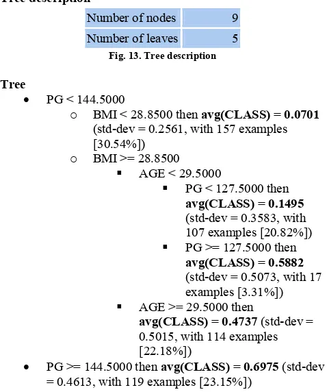
Tree description
Number of nodes 9
Number of leaves 5
Fig. 13. Tree description Tree
PG < 144.5000
o BMI < 28.8500 then avg(CLASS) = 0.0701
(std-dev = 0.2561, with 157 examples [30.54%])
o BMI >= 28.8500
AGE < 29.5000
PG < 127.5000 then
avg(CLASS) = 0.1495 (std-dev = 0.3583, with 107 examples [20.82%])
PG >= 127.5000 then
avg(CLASS) = 0.5882 (std-dev = 0.5073, with 17 examples [3.31%])
AGE >= 29.5000 then
avg(CLASS) = 0.4737 (std-dev = 0.5015, with 114 examples [22.18%])
PG >= 144.5000 then avg(CLASS) = 0.6975 (std-dev
= 0.4613, with 119 examples [23.15%])
Regression algorithm splits the data set into growing and pruning set. Here a two step algorithm was used. In the first step, a maximal tree was built that fits the possible growing set. In the second step, nested sub-trees were tested according to the cost-complexity principle, and RE was evaluated on the pruning set. It was noted that the optimal tree was selected on the pruning set and the simplest sub-tree was selected that had a performance near to the optimal tree.
Fig 14. Error reduction curve for growing set and pruning set
CONCLUSION
[image:5.612.330.534.453.554.2]information for medical researchers and doctors. In fact, the study with medical data by using the DM techniques is virtually an unexplored frontier which needs extraordinary attention. The results of the present investigation suggest that (i)the extraordinary behavior of outliers facilitates the exploration of the valuable knowledge hidden in their domain and help the decision makers to provide improved, reliable and efficient healthcare services (ii)medical doctors can use the present experimental results as a tool to make sensible predictions of the vast medical databases and finally(iii)a thorough understanding of the complex relationships that appear with regard to patient symptoms, diagnoses and behavior is the most promising area of outlier mining. In order to carry out this experiment on outlier detection, the Pima data set was used in the simulation carried out by TANAGRA. A total of 193 outliers have been detected for the statistics namely leverage, R-standard, R-student, DFFITS, Cooks’D and covariance ratio.
REFERENCES
Ben-Gal I.,Maimon O. and Rockach,L. (Eds.) 2005. Data Mining and Knowledge Discovery Handbook: “A Complete Guide for Practitioners and Researchers," Kluwer Academic Publishers, ISBN 0-387-24435-2.
Kristin B. DeGruy, 2000. Healthcare Applications of knowledge discovery in databases, JHIM, vol 14, no.2. Barnett, V. and Lewis, T. 1994. Outliers in Statistical Data.
John Wiley & Sons.
Fawcett, T. and Provost, F.1997. Adaptive fraud detection, Data Mining and Knowledge Discovery, 1, 3, pp. 291-316. Hawkins, D. 1980. Identification of Outliers, Chapman and
Hall: London.
Johnson, R.A. and Wichern, D.W. 2002. Applied Multivariate Statistical Analysis, India: Pearson Education.
Penny,K.L. and Jolliffe,I.T. 2001. A comparison of multivariate outlier detection methods for clinical laboratory safety data. The Statistician, 50, 3, pp. 295-308. Rajeeb Dey and Vaibhav Bajpai, Gagan Gandhi and Barnali
Dey, 2008, Application of Artificial Neural Network technique for Diagnosing Diabetes Mellitus, IEEE Region 10 Colloquium and the Third ICIIS, PID number 155,1-4. Siti Farhanah Bt Jaafar and Darmawaty Mohd Ali, 2005.
Diabetes Mellitus Forecast Using Artificial Neural Network, Asian Conference on Sensors and the
International Conference on new Techniques in
Pharmaceutical and Biomedical Research, pp.135 – 139. Varun kumar, Dharminder Kumar, R.K. Singh. Aug 2008.
Outlier mining in Medical databases. IJCSNS, Vol.8, No.8,