Contents lists available atScienceDirect
International Journal of Mechanical Sciences
journal homepage:www.elsevier.com/locate/ijmecsci
A generalisation of the Hill's quadratic yield function for planar plastic
anisotropy to consider loading direction
R.P.R. Cardoso
a,⁎, O.B. Adetoro
b aBrunel University London, Uxbridge, UB8 3PH London, UK bUniversity of the West of England, BS16 1QY Bristol, UKA R T I C L E I N F O
Keywords:
Quadratic yield function NURBS
Planar anisotropy R-values Flow stresses Earing profile Cup drawing
A B S T R A C T
In this work, a new generalised quadratic yield function for plane stress analysis that is able to describe the plastic anisotropy of metals and also the asymmetric behaviour in tension-compression typical of the Hexagonal Closed-Pack (HCP) materials, is developed. The new yield function has a quadratic form in the stress tensor and it simultaneously predicts the r-values and directionalflow stresses, which is shown to agree very well with experimental results. It also accurately describes the biaxial symmetric stress state which is fundamental for the accurate modelling of aluminium alloys. The new quadratic yield function represents the non-symmetric biaxial stress state by performing a linear interpolation from pure uniaxial loading to a biaxial symmetric stress state. The main advantages of this new yield function is that it can be used for the modelling of metals with any crystallographic structure (BCC, FCC or HCP), it only hasfive anisotropic coefficients and also that it is a simple quadratic yield criterion that is able to accurately reproduce the plastic anisotropy of metals whilst using an associatedflow rule.
1. Introduction
Material modelling is very important not only for the development of new metal alloys but also for the simulation of manufacturing processes. Within material modelling, plasticity plays a fundamental role and its description is essential for the accurate design of manu-facturing processes. In plasticity, yield functions are critical because they provide the yielding point of the material and also when used within an associatedflow rule scheme, they describe the plasticflow of the metal accurately. One of the first yield functions for plastic anisotropy was developed in the pioneer work by Hill (1948) [20]. Hill developed a quadratic yield function with anisotropic coefficients that could either predict the r-values or directionalflow stresses, but never both simultaneously. Moreover, Hill's original yield function does not include the effect of the biaxial symmetric stress and so it is not accurate in the modelling of aluminium alloys. Many posteriori yield functions[2–6]were developed after Hill's and the coefficients of these yield functions were designed to include the biaxial symmetric stress effect. Whilst the equi-biaxial flow stress has been defined in these functions, none of them have characterised the coefficients for the unsymmetric biaxial stress state between pure uniaxial loading and equi-biaxial loading.
The predominant deformation mechanism in Face-Cubic-Centred metals (FCC) such as aluminium alloys, is deformation by slip in the
crystallographic slip systems, which is basically a consequence of the movement of dislocations. In FCC materials, compressive and tensile strengths are virtually identical and yielding is not influenced by the hydrostatic pressure as well. The yield surface of such materials is usually represented adequately by an even function of the principal values of the deviatoric stresses (e.g. Hershey[19]and Hosford[21]). Hexagonal Close-Packed (HCP) materials, such as magnesium and titanium alloys, have less active slip systems at low/room temperatures but they have additional twinning systems that accommodate plastic deformation by a different mechanism known as twinning or distortion of the lattice. Twinning is a polar deformation mechanism (it only develops in one direction) and this is the main reason for the asymmetric behaviour observed on HCP alloys in tension-compression. For the description of incompressible plastic anisotropy, many yield functions have been suggested based on the isotropic hardening assumption (Hill[20], Barlat and Lian[2], Barlat et al.[3], Karafillis and Boyce[23]). Among them, Cazacu and Barlat[10]introduced a general formulation which originated from the rigorous theory of representation of tensor functions. However with this approach, the conditions for the convexity of the yield surface are difficult to derive and impose. The convexity has a physical basis and, in addition, this property ensures numerical stability in computer simulations. For this reason, a particular case of this general theory, which is based on linearly transformed stress components has received more interest from
http://dx.doi.org/10.1016/j.ijmecsci.2017.04.024
Received 31 January 2017; Received in revised form 28 March 2017; Accepted 24 April 2017 ⁎Corresponding author.
Available online 27 April 2017
0020-7403/ © 2017 The Authors. Published by Elsevier Ltd. This is an open access article under the CC BY license (http://creativecommons.org/licenses/BY/4.0/).
the metal forming and material modelling communities in general. Barlat et al. [3] applied this method to a full stress state in an orthotropic material and Karafillis and Boyce [23] generalised it as the so-called isotropic plasticity equivalent theory with a more general yield function and a linear transformation that can accommodate lower material symmetry.
Cazacu et al.[11]proposed a criterion based on a linear transfor-mation that accounts for the strength-differential effect, particularly prominent in Hexagonal Closed-Pack (HCP) materials, with the work being extended in Plunkett et al. [31]and Plunkett et al. [30] by including the effect of texture development in the yield function. Barlat et al. [5,6] later introduced two linear transformations which were applied on the sum of two yield functions in the case of plane and general stress states, in order to improve the accuracy of the functions by Cazacu et al.[11], Plunkett et al.[31]and Plunkett et al.[30]in the modelling of the anisotropic behaviour of aluminium sheets. Bron and Besson [8] further extended Karafillis and Boyce's approach to two linear transformations. These recently proposed yield functions include more anisotropy coefficients and therefore give a better description of the anisotropic properties of a material. Although the mathematical formulations are complex and very heavy from a computational point of view. These reported developments in yield functions have been particularly important for the study of the formability of sheet metals as shown in the works of Kuroda and Tvergaard[25], Stoughton and Yoon[36], Lou et al.[28]and Dasappa et al.[14].
Apart from the phenomenological studies listed above, another approach for the prediction of plastic anisotropy and strain hardening is the one based on polycrystal plasticity models. Commercial aluminium and magnesium alloys such as the aluminium AA6022 and AA2090 and the magnesium AZ31B used in this paper and used generally in forming operations, are polycrystalline materials composed of numerous grains each with a given lattice orientation with respect to macroscopic axes. At low temperatures, metals and alloys deform by dislocation glide or slip on given crystallographic planes and directions thereby producing microscopic shear deformations (Kocks et al. [24]). Therefore, the distribution of grain orientations and crystallographic texture in gen-eral, play an important role in the study and in the modelling of plasticity. Due to the geometrical nature of slip deformations, strain incompatibilities usually arise between grains thereby producing micro-residual stresses, which from a macroscopic point of view, can lead to the well-known Bauschinger effect. Slip results in gradual lattice rotation where dislocations accumulate at micro-structural barriers, increasing the slip resistance and consequently strain hardening. There is also another crystallographic deformation mechanism that is very typical of HCP materials which is the twinning. Proust et al. [32] developed the modelling of texture, twinning and hardening evolution of hexagonal materials by using the well-known Visco-Plastic Self-Consistent (VPSC) approach (Lebensohn and Tome [26]), where the interaction between a grain and its surrounding effective medium is taken into account. Polycrystal models can be used in multi-scale simulations of metal forming operations, but they are usually expensive in computational time.
Some noteworthy studies that use dislocation motion, micro-struc-tural grain size and shape data for the prediction of the yield strength of metallic alloys include the studies by Esmaeili et al.[17]and Balogh et al.[1], while some other studies perform a macroscopic study on the anisotropy of aluminium sheets from the consideration of morphologi-cal texture and crystallographic texture evolution (Choi et al. [12]). Polycrystal modelling aspects have been treated in a large number of publications and books such as in Kocks et al.[24], Gambin[18]and Dawson [15]. More recently, crystallographic plasticity has been extensively used in several numerical simulations, because it naturally predicts texture evolution and anisotropy, Bauschinger effect, transient behaviour and permanent softening. However, their computational cost is still prohibitive when compared to the use of phenomenological constitutive models.
Most of the early developed phenomenological yield potentials (e.g. von-Mises[38]and Hill's[20]) are quadratic in the stress tensor. These yield potentials were mainly designed from distortion energy balance equations, and they were developed primarily for steel alloys, with Hill's 1948[20]going a step further by including plastic anisotropy in the potential. It is widely accepted that these potentialsfit the yield locus very well for steel, but are unable to accurately predicting the anomalous behaviour of aluminium alloys (Dodd and Caddell[16]), especially in reproducing the yield locus on the vicinity of the symmetric biaxial stress state. There are two ways of accurately model aluminium alloys: i) by using non-quadratic yield functions with associatedflow rules; ii) by using quadratic yield functions with non-associatedflow rules (Stoughton and Yoon[37]), where in this case a plastic potential needs to be defined for the plasticflow. The use of non-associatedflow rules allows for the use of simpler yield potentials, such as the quadratic potential of Hill 1948 [20], but a second plastic potential needs to be used for the plasticflow. The use of two different potentials in the non-associated flow rule can however lead to difficulties during return mapping procedures, especially if the loci of the two potentials (yield and plastic potential) are of considerably different shapes. Considering however theflexibility in phenomenolo-gical modelling, it must be possible to develop a quadratic generalised yield function for simultaneously predicting r-values and directional
flow stresses accurately as opposed to the individual treatment that has been adopted so far. It also follows to say that it must be possible to simultaneously match the r-values and directionalflow stresses for any stress state, as for example under planar anisotropy assumption. This generalised yield function must be able to accurately predict the anomalous aluminium behaviour[16]and the symmetric biaxial stress state. Certainly, the yield function must be accurate for a wide range of cases and valid if, and only if, it is proven to be convex in the principal stress space. Therefore, the main ideas for the new yield function proposed in this paper are as follows:
•
A new quadratic yield function is developed for the simultaneous prediction of r-values and directionalflow stresses and its convexity is proven inAppendix Afor the case of proportional loading;•
This new model can simultaneously predict the r-values anddirectional flow stress accurately for any given angle from the rolling direction;
•
The biaxial symmetric flow stress is incorporated in this new quadratic yield function (this is detailed inSection 2.1). However, the biaxial r-value is not included in this formulation;•
It is postulated that the stress tensor changes in a linear manner between symmetric biaxial stress state and unaxial stress state, hence it is included in the new quadratic yield function in an interpolatory manner (details given inSection 2.1);•
Consequently due to this new quadratic yield function, it is possible to simultaneous predict r-values and directionalflow stress from the use of an associatedflow rule;The main objective of this research work is therefore to develop the yield function for plane stress analysis as general as possible so that it can work with associated flow rules for the modelling of planar anisotropy for both FCC and HCP materials and also that it is able to describe the asymmetric behaviour in tension-compression typical of HCP materials.
2. Model formulation
σ G H σ F H σ Hσ σ Nτ
F G H
= 3 2
( + ) + ( + ) − 2 + 2
+ +
xx2 yy2 xx yy xy2
(1) The coefficients F, G, H and N are designed to fit the r-values or, alternatively, the directional flow stresses but never both in simulta-neous. This is a major limitation in Hill's yield potential because both
fitting is required for the accurate modelling of planar plastic aniso-tropic metals. Hill's yield potential has however some great advantages which are its quadratic form and the simplicity of the model for the description of plastic anisotropy.
Therefore, a new yield function (YldParam) is defined as:
σ C u
G H σ F u H σ Hσ σ Nτ
F u G H
= 1 ( )
3 2
( + ) + [ ( ) + ] − 2 + 2 ( ) + +
a
xx2 yy2 xx yy xy2
(2) whereC ua( )is a new coefficient which defines the anisotropy in the yield stresses and the anisotropy for the r-values is conserved from the adaptation of coefficientFfrom the original Hill's model by making it variable. Both coefficients are a function of a parametric coordinateu, which represents the orientation of the loading direction when mea-sured from the rolling direction. This parametric variable u exists within the limits0.0 ≤u≤ 1.0, withu=0.0 defining the rolling direc-tion,u=0.125 being45°from the rolling direction,u=0.25 defining90° with the rolling direction andfinallyu=1.0 again defining the rolling direction. The coefficientC ua( )is designed tofit the yield stresses while the coefficientF u( ) is designed tofit the r-values. In this work, the functions for these two anisotropic coefficients are described from the use of Non-Uniform Rational B-Splines (NURBS) but they can also be described from the use of any other type of functions as far as the accurate values for the coefficients are conserved. The main reasons for the use of NURBS are essentially related to the local compact support of NURBS which is explained in more detail later in this manuscript. It is also demonstrated inAppendix Athat the new yield potential for plane stress analysis delivers a convex yield locus, which is a fundamental prerequisite for a stable stress integration procedure in elasto-plastic material modelling. The Hill's coefficientsH,GandNare obtained from the experimental r-values at0°,45°and90°from the rolling direction [20]:
H r
r
G r
N r r r
r r
= 2 1 +
= 2 1 +
= 2( + ) (2 + 1) 2 (1 + )
0
0
0
0 90 45
90 0 (3)
The r-value anisotropic coefficientF u( )will be calculated from the use of a Non-Uniform Rational B-Spline (NURBS) approximation on the parametric coordinate u. For that purpose, it will be necessary to calculatefirst the r-value anisotropic coefficientFat every15°from the rolling direction and then use the NURBS approximation to build a function F u( ) that can generate the F-coefficient for any loading orientation θ. The Hill's 1948 [20]formulae for this coefficient can be used as presented in the following equation:
F θ H θ θ G θ θ r θ N θ θ
θ θ r θ
( ) = (1 − 4 sin cos ) − (sin cos + cos ) + 2 sin cos sin cos + sin
θ
θ
2 2 2 2 2 2 2
2 2 2
(4) This function forF θ( )is singular at0°and so the following alternative function was used for the calculation of the coefficient at0°:
F r
r r
(0°) = 2 (1 + )
0
90 0 (5)
For the NURBS approximation for bothC ua( ) andF u( )the following relation between the angle from the rolling direction and the para-metric coordinateuis necessary:
θ= 2πu (6)
and the angleθcan be easily obtained from the Mohr's circle or from the equation for the principal directions from plane stress analysis:
θ τ
σ σ
tan (2 ) = 2 −
xy
xx yy (7)
The coefficientC ua( )will be calculated from the new yield function from Eq.(2)and from the yield stressesσθdefined at every15°from the rolling direction. From the stress transformation of the uniaxial loading to the anisotropic axes we can get:
σ σ θ
σ σ θ
τ σ θ θ
= cos = sin = cos sin
xx θ yy θ xy θ 2 2 (8) and after replacing Eq.(8)into Eq.(2)the following is obtained for coefficientC ua( ):
C u σ σ
G H θ F u H θ N H θ θ
F u G H
( ) = 3 2
( + ) cos + [ ( ) + ] sin + 2 ( − ) cos sin ( ) + +
a θ
4 4 2 2
(9) whereσ
σ
θ is the normalisedflow stress at directionθfrom the rolling direction obtained from experimental data.
2.1. Incorporation of the biaxial symmetricflow stress
The model defined so far does not consider the biaxial symmetric yield stress. If the stress tensor deviates considerably from the uniaxial stress state (defined by the principal stresses σ1> 0 and σ2= 0 for tension or σ2< 0 and σ1= 0 for compression), the differences in the accuracy can be substantial and this is more severe when the stress tensor is closer to the biaxial symmetric stress state. So, the incorporation of the biaxial symmetric flow stress in the model is important.
A generalised yield function in the normalised principal space, σ σ1/ −σ σ2/ is shown inFig. 1and for each quadrant, the Mohr's circle with the possible loading directions is depicted. In thefirst quadrant (σ1> 0andσ2> 0) it is possible to have a uniaxial tensile stress tensor defined with angleθfrom the rolling direction, a biaxial tensile stress state and a biaxial symmetric tensile stress state, which is not represented by a circle but rather by a dot (σ1=σ2). In the second and forth quadrant, the applied loading leads to a shear stress state (σ1> 0andσ2< 0orσ1< 0andσ2> 0) and in the third quadrant it is possible to have a uniaxial compressive stress tensor defined with angle θfrom the rolling direction, a biaxial compressive stress state and a biaxial symmetric compressive stress state.
The material calibration in most of well-known yield functions requires several mechanical tests: uniaxial tests for r-values and directionalflow stresses and mechanical tests for the equi-biaxial stress (or bulge test) and the disk compression for the equi-biaxial r-value. The results from these tests are then included in optimisation algo-rithms for the calculation of the anisotropic coefficients, a procedure that is very common for example with the Barlat yield functions for aluminium[5,6]. The stress tensor as one transits from a symmetric biaxial state through an unsymmetric biaxial state to a uniaxial stress state remains unknown, however it is postulated in this work that a linear variation is valid. Hence an interpolation scheme is thus proposed between a uni-axial stress and a biaxial symmetric flow stress. The Mohr circle fromFig. 2shows how far the stress state is from uniaxial stress conditions, or alternatively, how close it is to symmetric biaxial stress state. Ifσ2= 0we have uniaxial stress state and ifσ2=σ1 we then have symmetric biaxial stress state. We can therefore inter-polate between these two stress states by introducing a parameterβ defined in Eqs. (11) and (12) that represents the deviation from a symmetric biaxial stress state.
C u β( , ) =β C u· a( ) + (1 − ) ·β C ub( ) (10) where:
β σ σ
σ
= 1− 2
1 (11)
for biaxial tension and:
β σ σ
σ
= 2 − 1
2 (12)
for biaxial compression. For β= 0 we have symmetric biaxial stress state and forβ= 1we have uniaxial stress. For0 <β< 1we have a stress state somewhere between uniaxial and symmetric biaxial.
Thus, the new quadratic yield function from Eq.(2)becomes:
σ
C u β
G H σ F u H σ Hσ σ Nτ
F u G H
= 1
( , ) 3 2
( + ) + [ ( ) + ] − 2 + 2
( ) + +
xx2 yy2 xx yy xy2
(13)
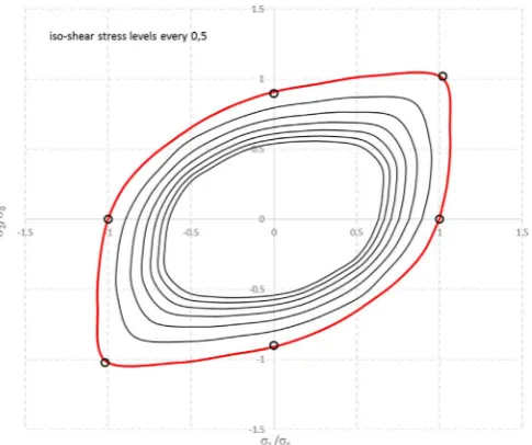
2.2. Iso-Shear contours for the yield locus
Another coefficientC uc( )can be introduced for greaterflexibility of the yield locus for different (non-zero) iso-shear contour levels. This new coefficient can be added to the linear interpolation for the biaxial symmetricflow stress as described inSection 2.1. It is associated with the shear stressτxyin the following way:
σ
C u β C u
= 1
( , ) + ( ) 3 2×
×
c τ
σ
G H σ F u H σ Hσ σ Nτ
F u G H
( + ) + [ ( ) + ] − 2 + 2
( ) + +
xy
xx yy xx yy xy
0
2 2 2
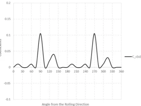
[image:4.595.125.477.61.309.2](14) whereσ0is the initial yield stress at 00with the rolling direction. An example for the coefficientC uc( )for the Al2090 aluminium alloy used in the example ofSection 5.1.2is depicted inFig. 3.
[image:4.595.39.290.351.501.2]Fig. 1.Yield function and Mohr's circles at different quadrants representing different loading directions.
Fig. 2.Mohr's circle for a generalised biaxial stress state.
[image:4.595.312.555.549.731.2]3. Non-uniform rational B-spline (NURBS) for the representation of the non-constant coefficients
NURBS have been used extensively in geometric modelling because it is able to represent curves and/or surfaces with high complexity in their shape. Piegl [29], Hughes et al. [22] and Bazilevs et al. [7] addressed the most fundamental properties of the NURBS basis func-tions, however the most important attributes for this work are listed below:
1. They form a partition of unity, i.e.:
∑
N ( ) = 1,u u∈U= [ ,u u ];J m J p m p =1
1 + +1
(15)
2. The support of eachNJp( )u is compact and contained in[ ,u uJ J p+ +1]; 3. The basis functions are non-negative, that is,∀u→NJ( ) ≥ 0u
p ; 4. Affine invariance.
3.1. Knot vector
An open knot vector is a set of non-negative parametric coordinates which are repeatedp+ 1times at the beginning and at the end of the vector (p is the order of the polynomial basis functions). For one-dimensional basis functions of orderp, the following generic open knot vector can be defined:
U= { , …,u1 up+1, …,um+1, …,um p+ +1} (16) wheremis the number of control points or basis functions. The basis functions of orderphavep− 1continuous derivatives. More than one knot can be considered at the same parametric coordinate and it is thus referred as a repeated knot. An important property of repeated knots is that the continuous derivative of their basis functions is decreased by the number of times the knot is repeated. Also, the basis functions are interpolatory only if the knot's multiplicity is the same as the polynomial's orderp[29]. For this quadratic yield function, the knot vector is defined for the limits0.0 ≤u≤ 1.0, whereu=0.0 corresponds to an angleθ= 0°with the rolling direction andu=1.0 corresponds to an angle of θ= 360° with the rolling direction. For instance, for a quadratic degree in the NURBS basis functions (p=2) we have the following knot vector:
U= {0.0, 0.0, 0.0, 1.0, 1.0, 1.0} (17)
3.2. Basis functions, control points and approximation for the coefficients
For a specific local parametric coordinate u from an open knot vector and for a degree pof the polynomial, the basis functions are obtained recursively from the following formulae[13,22,29]:
N u u u
u uN u
u u
u uN u
( ) = − − ( ) + − − ( ), I p I
I p I
I
p I p
I p I
I p
+
−1 + +1
+ +1 +1
−1
(18) whereIis the index for the basis functions. The formula for the basis functions in Eq.(18)must be initialised from piecewise basis functions corresponding to the polynomial orderp=0, i.e.:
⎧ ⎨ ⎩
N u if u u u
otherwise
( ) = 1 ≤ <
0
I
I I
0 +1
(19) In this work, NURBS approximation functions are defined for the coefficientsC ua( ),C ub( )andF u( )as follows:
∑
∑
∑
F u N u W F
W
C u N u W C
W
C u N u W C
W
( ) = ( )
( ) = ( )
( ) = ( )
I
I I I
a
I
I I aI
b
I
I I bI
(20) with:
∑
W= N u W( )
I
I I
(21) We will use the weightsWIequal to 1.0 and because of the partition of unity property of the NURBS basis functions (∑IN uI( ) = 1), the NURBS approximations are reduced to:
∑
∑
∑
F u N u F
C u N u C
C u N u C
( ) = ( ) ( ) = ( ) ( ) = ( ) I I I a I I aI b I I bI (22) In Eq. (22), N uI( ) are the NURBS basis functions which are used to approximate the coefficientsF u( ),C ua( )andC ub( ).FI,CaIandCbIare the control points, whose definition can be found in the works of Piegl and Tiller [29]. A detailed description on how these control points are obtained for the current work can be found inAppendix B. The use of the same basis functions for all coefficients is thefirst advantage of the use of NURBS. Another important advantage of using NURBS is that they have local compact support, i.e. for a particularuin the parametric domain, onlyp+ 1control points in the domain of influence need to be used because outside of this domain of influence all other NURBS approximation functions are zero. In this work,p=2 is used for the NURBS basis functions.
4. Return mapping procedure
From a phenomenological point of view, the plastic flow can be interpreted as an irreversible process in a material body, typically a metal, characterised in terms of the history of the strain tensorϵand two additional variables: the plastic strainϵpand a suitable set of internal variablesα often referred to as hardening parameters. Conventional constitutive laws which represent plastic deformation of metals are typically described by considering three parts: yield func-tions, stress-strain (or hardening) functions and the associated normal-ity flow rule. The yield function describes yield stresses in general deformation states, which are relative values measured with respect to a reference yield stress. The stress-strain function represents the work-hardening behaviour of the reference stress, which is usually a uniaxial or balanced biaxial tension stress.
The notion of irreversibility of plastic flow is expressed by the following equations of evolution for the set of internal variables{ϵp, }α, calledflow rule and hardening law, respectively:
ϵ σ α
α σ α
γ γ r H ̇ = ̇ ( , ) ̇ = ̇ ( , ) p (23) wherer( ,σ α)andH( ,σ α) are prescribed functions which define the direction of plasticflow and the type of hardening. The parameterγ̇is a non-negative function, called the consistency parameter, which is assumed to obey the following Kuhn-Tucker complementary conditions:
σ α σ α γ
f γf
̇ ≥ 0 ( , ) ≤ 0
̇ ( , ) = 0 (24)
σ α
γḟ ( , ) = 0 (25)
The consistency requirement allows the unloading to an elastic stress state (ḟ ( , ) < 0σ α and consequently γ= 0) and it also demonstrates that the stress tensor is always located at the yield surface (ḟ ( , ) = 0σ α
and soγ> 0).
When using associated flow rule, the plastic strain tensor can be obtained directly from the yield potential as follows:
ϵ σ
γ σ
= Δ ∂ ∂
p t Δ
(26) When using the forward-Euler scheme for return mapping proce-dures[9,34,39,40], the time steps are assumed to be small enough for the coefficientsC ua( )andF u( )to be considered constant during return mapping. However, for larger time steps, the derivative of the equivalent yield stress obtained from the following chain rule can be used: ⎛ ⎝ ⎜ ⎞ ⎠ ⎟ ϵ
σ σ σ
γ σ σ
C u C u u u σ F u F u u u
= Δ ∂ ∂ + ∂ ∂ ( ) ∂ ( ) ∂ ∂ ∂ + ∂ ∂ ( ) ∂ ( ) ∂ ∂ ∂ p t Δ (27) where:
∑
∑
C u u dN u du C F u u dN u du F ∂ ( ) ∂ = ( ) ∂ ( ) ∂ = ( ) I I I J J J (28) and∂ /∂u σ is obtained from the derivative of Eqs. (6) and (7). If an associatedflow rule is used and if the return mapping of the trial stress state to the yield surface is considered to be along the path with the closest distance to the yield function then the derivative∂ /∂u σ can be assumed to be zero and so the plastic strain tensor from Eq.(27)reduces to:ϵ σ
γ σ
= Δ ∂ ∂
p t Δ
(29) which simplifies considerably the return mapping procedure.
In the forward-Euler scheme for return mapping, the stress tensor can be corrected from the predictor stage as follows:
σ σ ϵ σ
σ
γ σ
D D
= − = − Δ ∂
∂
t+Δt trial Δt p trial
(30) The r-value is by definition obtained from the plastic strain in the width direction over the plastic strain along the thickness direction, i.e.:
r = ϵ
−(ϵ + ϵ )
θ θ π p θ p θ π p + /2
+ /2 (31)
and using Eq.(26)and the stress transformation Eq.(8), the following result for the r-value can be obtained:
r H N F u G H θ θ
F u θ G θ
= + [2 − ( ) − − 4 ] sin cos ( ) sin + cos
θ
2 2
2 2 (32)
where it can clearly be seen that the r-value can be matched by adjusting the parameterF u( )accordingly.
5. Validations and discussion
For validating the proposed quadratic yield function, single element uniaxial simulations are performed along every 15 degrees from the rolling direction for different case studies. The predicted r-values and
flow stresses are compared with experimental results and with predic-tions from different yield criteria such as Hill's 1948,“yld91”(Barlat and Lian[3]),“yld96”(Barlat et al.[4]),“yld2000”(Barlat et al.[5]), “CPB06ex2”(Cazacu et al.[11]) and the new quadratic yield function, “YldParam”, proposed in this paper.
Fig. 4shows the procedure used for the prediction of r-values. As shown inFig. 4, a1 × 1 × 0.1 mmsingle element is elongated and then
unloaded to eliminate the elastic deformation, since r-value is a plastic property. An additional boundary condition to impose equal vertical displacement was also considered for the nodes on the top of the element square.
The predicted r-value for an angleθwith the rolling direction is defined as:
r = − ϵ
ϵ + ϵ
θ 22
22 11 (33)
where: ⎛ ⎝ ⎜ ⎞ ⎠ ⎟ ⎛ ⎝ ⎜ ⎞⎠⎟ dx x dy y
ϵ = ln 1 +
ϵ = ln 1 +
11
22
(34) This simple one-element test is going to be used with the different yield criteria listed above for the assessment of the accuracy of the different yield models for plastic anisotropy. These validations are going to be performed for three different alloys (case studies): two aluminium alloys AA6022 and AA2090, for weak and strong plastic anisotropy validations, and also for the AZ31B Mg alloy, where the main objective is to demonstrate the generality and accuracy of the new yield function in describing the plastic anisotropy as well as the asymmetry in tension-compression.
5.1. r-values and directionalflow stresses for FCC materials
5.1.1. The AA6022 aluminium alloy
The Young's modulus and Poisson's ratio used were: E= 70000.0 MPaandν= 0.3, respectively. The following Voce's curve was used for strain hardening:
σ= 328.36 − 194.5 · exp (−10.941 · ϵ )p
(35) InFig. 5, the yield locus projected on the zero shear stress plane, τxy= 0, is shown for Hill's 1948, Barlat yld2000 and the new quadratic yield function (the stresses are normalised from the uniaxial stress at 0 degrees (σ0)). It can be seen that the new yield function delivers a yield locus which is almost coincident with the yield locus from Barlat et al. [5], yld2000, but considerably different from the yield locus of Hill's 1948 yield criterion. It can be also seen that the symmetric biaxial yield stress was captured very well with this new yield function.
InFig. 6, the yield locus contours for every 0.5 values of shear stress is shown, where the shape of the different yield locus is projected at different shear stress planes.Fig. 7shows a plot of coefficientsF u( ),G, H, N, C ua( ) andC ub( ) as a function of the angle with the rolling direction. The coefficientsG,HandNare constants but the coefficients F u( ), C ua( ) and C ub( ) are not constant, they are function of the parametric variable u which in turn represents the angle measured from the rolling direction. The plots for the non-constant coefficients is symmetric about180°, as expected for this alloy because there is no difference in its behaviour when in tension compared to when in compression. Another important aspect that is noteworthy from the plot of the coefficients inFig. 7is the comparison betweenC ua( )andC ub( ). It can be seen that these two coefficients are the same at every orientation except at orientations in the vicinity of the symmetric biaxial stress region. This was also expected considering the coefficientC ua( ) was designed tofit the uniaxial yield (flow) stresses, while the coefficient C ub( )was designed for the symmetric biaxial stress state.
coefficients for Barlat yield functions were designed tofit r-values at0°, 45°and90°only and so we cannot expect a perfect prediction for all other directions. On the contrary, the coefficientF u( )for the new yield function was designed tofit r-values at every direction and this explains the better accuracy of the newly proposed model.
InFig. 9the predictions for the normalisedflow stresses at every15° from the rolling direction are compared. Again, the comparison is made for the same yield models used for the r-values prediction and a comparison is also made with experimental results. Theflow stresses for the new quadratic yield function were obtained following the deriva-tion from Eq.(9), i.e.:
σ σ C u
F u G H
G H θ F u H θ N H θ θ
= ( ) 2 3
( ) + +
( + ) cos + [ ( ) + ] sin + 2 ( − ) cos sin θ
a 4 4 2 2
(36) All yield criteria deliver normalised flow stresses very close to experimental results with the exception of Hill's 1948 yield criterion. It is also fair to say that the disparity for the Hill's results for the normalised yield stresses is expected because in this work the Hill coefficients were designed tofit the r-values and not the normalised
flow stresses.
5.1.2. The Al2090 aluminium alloy
The aluminium alloy AA6022 does not represent an alloy with a
[image:7.595.52.498.57.462.2]strong plastic anisotropy. This can be clearly seen fromFigs. 8 and 9for the low amplitude for both the r-values and for the normalisedflow stresses. The aluminium alloy AA2090, on the contrary, shows a very strong plastic anisotropy with high amplitudes or range for both r-Fig. 4.Definitions for r-value calculation.
Fig. 5.Yield locus for AA6022: comparison between Hill's 1948, yld2000 and the new yield function (τxy= 0). Stresses normalised with the yield stress at 0 degrees (σ0).
[image:7.595.305.558.65.464.2]Fig. 6.Yield locus contours for AA6022 projected on shear planes for every 0.5 shear stress.
[image:7.595.43.293.82.459.2] [image:7.595.309.554.501.678.2]values and normalised flow stresses and thus it represents a higher challenge for the newly proposed quadratic yield function.
The Young's modulus and Poisson's ratio used in this validation were:E= 70000.0 MPaandν= 0.3, respectively. The following Power law was used for strain hardening:
σ= 646.0 · (0.025 + ϵ )p0.227 (37) In Fig. 10, the yield locus projected on the zero shear stress plane, τxy= 0, for the Hill's 1948 and the new quadratic yield function is shown together with some experimental results. The stresses were normalised with the uniaxial stress at 0 degrees (σ0). It can be seen that the new yield function delivers a yield locus which matches excellently well with the experimental results. It is quite interesting to see the difference in the yield locus when compared with the Hill's 1948 yield function; Hill's 1948 does not fit the biaxial symmetric flow stress accurately as expected because it does not have included the equi-biaxial stress in his model. On the contrary, the equi-equi-biaxial yield stress was very well captured with this new quadratic yield function. Another noteworthy point is the ability of predicting the aluminium's behaviour
from the use of quadratic yield functions with an associatedflow rule. It is well-agreed up till now that if an associatedflow rule is used with aluminium alloys than the yield criterion needs to be non-quadratic, otherwise erroneous predictions for r-values and/or normalised yield stresses should be expected. Alternatively, if a non-associatedflow rule is to be used, then a quadratic yield potential, such as Hill's 1948, should be able to accurately represent the aluminium's behaviour. The main reason is that with a non-associatedflow rule the yield potential can be used to match the normalised yield stresses while the plastic potential can be used to match the r-values. Barlat yield functions (yld91, Barlat et al.[3], yld96, Barlat et al.[4]and yld2000, Barlat et al.[5]) were all designed to be non-quadratic yield functions as well as the CPB06ex2 yield function of Cazacu et al.[11].
InFig. 11the yield locus contours for every 0.5 values of shear stress is shown. InFig. 12, a plot of the coefficientsF u( ),G,H,N,C ua( )and
[image:8.595.138.456.54.282.2]C ub( ) is shown as a function of the angle from the rolling direction. Again, the coefficientsG,HandNare constant but the coefficientsF u( ), C ua( )andC ub( )are not. The plots of these two non-constant coefficients show again a symmetry at180°. It is also worth noting for this example Fig. 8.Comparison between measured and predicted r-values for the AA6022 aluminium alloy.
[image:8.595.140.454.514.731.2]the comparison betweenC ua( ) andC ub( ) as discussed in the previous section but, although, the deviation is not as prominent for this alloy because the effect of the symmetric biaxial stress is much less when compared to that of the AA6022 aluminium alloy.
Fig. 13shows the comparison between the predicted r-values and experimental results. It can be seen that the predictions for the r-values from the new quadratic yield function match the experimental results for every orientation very well, with a slight deviation at60°. Hill's 1948 gives good agreement at0°,45°and90°and the same can be said for the Barlat yield functions yld91, yld96 and yld2000. The prediction of r-values for the Barlat yield functions at every15°from the rolling direction is not as good as the new quadratic yield function because the coefficients for Barlat yield functions were designed tofit r-values at0°, 45°and90°only and so we cannot expect a perfect prediction for all other directions. On the contrary, the coefficient F u( ) for the new quadratic yield function was designed tofit r-values at every direction and this explains the better accuracy of the proposed model.
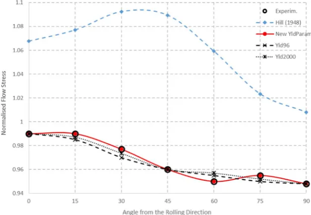
All yield criteria shown deliver normalisedflow stresses very close to experiments with the exception of Hill's 1948 yield criterion as seen inFig. 14. It can also be said that the Barlat yield criteria (yld91 and yld96) struggles a bit to match the experimental normalisedflow stress at30°. As discussed in the previous section, it is fair to say that the disparity for the Hill's results for the normalised yield stresses is expected because Hill coefficients in this work were designed to fit the r-values, not the normalisedflow stresses. If the Hill coefficients had beenfitted for the normalised yield stresses we should then expect a much better prediction of the Hill model for the normalised yield stresses but then the prediction for the r-values would be worst.
5.2. Cup drawing for earing prediction
The new yield function was also tested for a cup drawing simulation for the prediction of the cup earing profile for an Al 2090-T3 aluminium alloy.
Fig. 15depicts the geometry for the die tools and for the blank sheet. The following dimensions were used in our analysis:
•
Punch diameter:Dp= 97.46 mm•
Punch profile radius:rp= 12.70 mm•
Die opening diameter:Dd= 101.48 mm•
Die profile radius:rd= 12.70 mm•
Blank radius:Db= 158.76 mmThe material properties used in the analysis are given below:
•
Stress-strain curve characteristics:σ= 646(0.025 + ϵ)0.227(MPa)•
Initial sheet thickness:t0= 1.6 mm•
Coulomb coefficient of friction: 0.1•
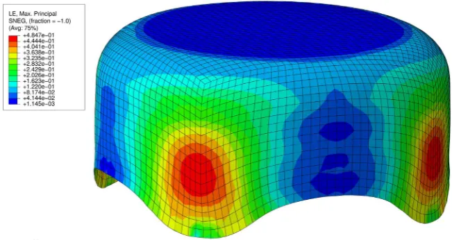
Blank holding force:22.2 kNThe cup drawing simulation was carried out in the commercial software ABAQUS and by using a user material subroutine“VUMAT” for the new yield function.Fig. 16depicts the deformed configuration and the earing profile for the cup after the cup drawing operation.
[image:9.595.44.286.54.258.2]InFig. 17the cup earing profile is compared for the experimental results from Yoon et al. [41], Yld96 without translation [41] (or without consideration of the strength differential effects) and the new yield function. For an orthotropic material, the cup height profile between 0 and 90 degrees should be the mirror image of the cup height profile between 90 and 180 degrees with respect to the 90 degrees axis. However, the measured earing profile slightly deviates from this condition and, according to Yoon et al.[41], this deviation might have occurred because the center of the blank was not aligned properly with the centers of the die and the punch during processing. The earing magnitude is in good agreement with the simulations of Yoon et al.[41] for the Yld96 without translation and also in reasonable agreement with Fig. 10.Yield locus for Al2090: comparison between Hill 1948, the new parametric yield
[image:9.595.44.287.304.507.2]function and experimental results.
[image:9.595.43.285.556.730.2]Fig. 11.Yield locus contours for Al2090 projected on shear planes for every 0.5 shear stress.
the measured result, but however, both Yld96 and the new yield function do not lead to the correct trend: the experimental cup height at 0 degrees is larger than that at 90 degrees, whereas the simulated results predict the reverse. Yoon et al. [41] and Yoon et al. [43] reported this to be a consequence of the cup drawing simulations being performed from coefficients based on the tensile test results. In their work, Yoon et al.[41]said that since the stresses in theflange area are nearly compressive in nature, the cup drawing simulations should also account for the compressive test results. In other words, they are suggesting that there is a strength differential effect that should have been considered during the material characterisation of the Al2090 aluminium alloy. It was shown in Yoon et al.[41]that if the strength differential effect was considered (Yld96 with translation of the yield surface) then a better agreement could be obtained with the experi-mental results. It is therefore more important to compare the results obtained with the new yield function with the results from the use of Yld96 without translation of the yield surface (both plotted inFig. 17)
Fig. 13.Predictions and experimental results for the r-values of the Al2090 aluminium alloy.
[image:10.595.309.554.310.454.2]Fig. 14.Comparison for predictions offlow stresses for the Al2090 aluminium alloy.
[image:10.595.140.456.503.730.2]as they properly reflect the material characterisation employed in the simulation.
For the Al2090-T3 alloy, Yoon et al.[42]demonstrated that a more accurate prediction of the r-value at 75 degrees should be reflected into a small ear around 15 degrees and so the earing profile should include six ears instead of four ears. This behaviour was not observed with the current model maybe due to the slight deviation of the r-value prediction obtained for 75 degrees from the rolling direction.
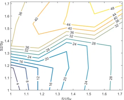
5.3. Iso-error maps
In this section we assess the accuracy of the return mapping procedure used in this work by means of the iso-error maps, as detailed in Simo and Hughes[34]. The new yield function developed in this work was designed to work with the semi-implicit or forward-Euler return mapping scheme, as detailed inSection 4 and as derived in a previous work of Cardoso and Yoon[9], where it is assumed that the trial stress state is not too far away from the yield locus or, in other words, the incremental time steps are considered to be sufficiently small enough. The iso-error maps presented in this section were constructed for the Al2090 alloy, whose yield locus has the shape as described in Fig. 10, including regions with high curvature, making the accuracy and even the convergence of the return mapping scheme much more complicated.
Three points on the yield surface were considered for the plotting of the iso-error maps: point A, corresponding to the uniaxial stress state; point B, which is a biaxial stress state; point C, which corresponds to the pure shear stress state. All of these points are schematically represented inFig. 18.
Without any loss of generality, the initial stress state for points A, B and C is the one corresponding to locations at the yield locus for the initial yield point. Subsequently, incremental stresses in the principal directions“S1”and“S2”are added and the return mapping scheme is applied for the assessment of the iso-error contours. There is the need to calculate the exact stress tensor for points A, B and C after return mapping and that is done in this current work by applying 10,000 infinitesimal stress increments between the yield locus and the yield locus for the trial stress state. The iso-error contourEis constructed from the following equation:
σ σ σ σ
σ σ
E= ( − *) : ( − *)
* : * × 100 (38)
whereσ*is the exact stress tensor andσis the stress tensor after return mapping.
[image:11.595.134.460.57.230.2] [image:11.595.140.453.525.730.2]The plots for the iso-error contours for points A, B and C inFigs. 19, 20 and 21, respectively, were constructed for S Sy1/ ≤ 1.75 and S2/Sy≤ 1.75, whereSyis the initial yield stress of Al2090 alloy. Because the return mapping scheme used in this work is a forward-Euler scheme Fig. 16.Al2090 deformed cup after drawing.
(traditionally used for explicit analysis), then if larger time steps (or larger S Sy1/ ratio) are used there is the chance of divergence in the return mapping scheme and that is even more critical for the high curvature yield locus of the Al2090 aluminium alloy. This was also proved to be the case when the Barlat yld2000 yield function was used
for the forward-Euler scheme in the work of Cardoso and Yoon[9]. Another aspect that is worth discussing is the computational performance of the return mapping scheme used. This was addressed by Cardoso and Yoon[9], however the return mapping scheme now comes together with a new yield function so it is worth considering the computational costs or benefits added by the new yield function to the return mapping procedure. When compared with the yld96 function used for the cup drawing for the earing profile of previous section, it can be said that there is the need to calculate the loading direction as in Eq.(7), however this is computationally inexpensive. The other major difference of this new yield function is the calculation of the plasticflow direction, where in this case we calculate the normal to the yield surface (derivative of the yield potential) by using B-Splines basis functions and the derivative of the B-Spline's basis functions for the anisotropic coefficients. When comparing with the yld96 yield function, the normal to the yield surface also has to be calculated and the derivatives of the yield potential, however, for the approximation of the coefficients for a particular loading direction, only the coefficients inside the local compact support of the B-Spline basis functions need to be considered. If the polynomials used for the B-Splines basis function have degree“p”then the size of the local compact support isp+ 1, so for a quadratic degree only three coefficients in the local compact support of the loading direction“u”need to be used. If we compare with more elaborated yield functions such as Barlat's yld2000, there are the advantages of the straightforwardness of obtaining the anisotropic coefficients as well as the simplicity for the calculation of the plastic
flow tensor for the normal to the yield surface. In the comparison study carried out for the Al2090 alloy, the differences for the computational performance of the return mapping scheme used for the new yield function and for the yld96 and yld2000 yield functions are barely undetectable.
5.4. r-values and directionalflow stresses for HCP materials
5.4.1. The AZ31B Mg alloy
[image:12.595.54.273.54.249.2]The last case study presented in this paper is for a HCP material, the AZ31B Mg alloy. Many yield functions were developed to account for the asymmetry in tension-compression for these alloys and amongst them we can distinguish the works of Cazacu et al.[10,11]and more recently the work of Soare and Benzerga [35]on the modelling of asymmetric yield functions. The main objective of this case study is to demonstrate that the newly proposed yield function for plane stress analysis is generalised enough to accurately predict the plastic aniso-tropy for this alloy as well as its asymmetric behaviour in tension-compression. The Young's modulus and Poisson's ratio used were: E= 42000.0 MPaandν= 0.35, respectively. The following Voce curve Fig. 18.Points A (uniaxial), B (biaxial) and C (pure shear) for the iso-error maps.
2 2 4 4 6 6 8 8 10 10 12 12 14 14 16 16 18 18 20 20 22 22 24 24 26 26 28 28 30 30 32 32 34 34 36
1 1.1 1.2 1.3 1.4 1.5 1.6 1.7
S1/Sy 1 1.1 1.2 1.3 1.4 1.5 1.6 1.7 S2/Sy
Fig. 19.Iso-error plot for point A (uniaxial stress state).
4 8 12
16 16 20 20 24 24 24 28 28 28 32 32 32 36 36 36 36 40 40 40 44 44 48
1 1.1 1.2 1.3 1.4 1.5 1.6 1.7
[image:12.595.322.542.54.236.2]S1/Sy 1 1.1 1.2 1.3 1.4 1.5 1.6 1.7 S2/Sy
Fig. 20.Iso-error plot for point B (biaxial stress state).
4 6 810 12 14 16 18 20 20 22 22 24 24 26 26 28 28 30 30 32 32 34 34 36 36 38 38 40 40 42 42 44 44 46
1 1.1 1.2 1.3 1.4 1.5 1.6 1.7
[image:12.595.58.272.279.453.2]S1/Sy 1 1.1 1.2 1.3 1.4 1.5 1.6 1.7 -S2/Sy
[image:12.595.56.274.484.659.2]was used for strain hardening: σ= 361.43 − 158.6 · exp (−9.74 · ϵ )p
[image:13.595.310.554.54.227.2](39) In Fig. 22, the yield locus for the Hill 1948 yield function, for Cazacu et al. [11]CPB06ex2 yield potential, for the newly proposed quadratic yield criterion (YldParam) and for the experimental results from Lou et al.[27]are presented. It can be seen that the proposed new yield function is able to predict accurately the asymmetry in tension-compression that is very typical of this alloy. The CPB06ex2 yield criterion is also extremely accurate but, as reported by Plunkett et al. [31], it requires the calculation of 18 anisotropic coefficients plus 2 additional coefficients to describe the asymmetry in tension-compres-sion, it is not a quadratic yield potential and it requires at least two linear transformations for the yield potential. InFig. 23it is shown the yield locus contours for every 0.5 values of shear stress. It shows the shape of the different yield locus when projected at different shear stress planes.
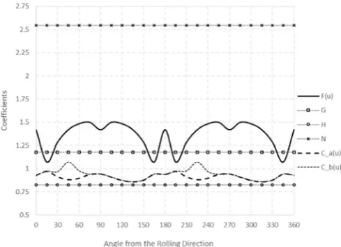
Fig. 24shows a plot of coefficientsF u( ),G,H,N,C ua( )andC ub( )as a function of the angle from the rolling direction. It is important to notice that for this case study the coefficientsG,HandNhave different values for tension and compression and so are not constant for the entire range of loading directions. The reason for the different distribution for these coefficients is due to the asymmetric behaviour of HCP alloys, which requires a separated calibration for the tension and compression domains. The plot for the coefficientsF u( ),C ua( )and
C ub( ) is not symmetric at180° due to the asymmetric behaviour in tension-compression of this particular Mg alloy. Also, regarding the coefficients C ua( ) and C ub( ) from Fig. 24, and in particular their comparison in the vicinity of the symmetric biaxial stress state, it can be said that the difference between the coefficients is higher in tension than it is in compression.
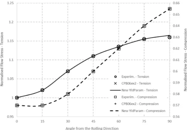
Fig. 25 shows the r-values predictions and comparisons with experimental results for both the tension and compression regions. The prediction from the new yield function is compared with Plunkett et al.[31]predictions based on the yield criterion CPB06ex2 of Cazacu et al.[11]. It can be seen that the CPB06ex2 yield criterion is just perfect in accurately predicting the r-values for both tension and compression regions. The new yield function is also great for the prediction of the r-values in tension and some slight deviations are seen for the r-values in compression, mostly for45°and75°. However, it is reasonable to say that these minor deviations are still good if we consider the fact that these predictions were obtained from the use of a quadratic yield potential. In regards to the normalised yield stresses from the plots inFig. 26, the conclusion is that both Cazacu et al.[11] CPB06ex2 yield potential and the newly proposed formulation deliver excellent agreement with the normalised yield stresses from experi-ments.
In this paper, the general definition or classification of a“quadratic planar anisotropic yield function”is adopted. This commonly refers to the exponent used directly in the stress components inside the yield criterion, which in the case of this new yield function is of degree two as in the original Hill's yield criterion [20]. All non-quadratic (higher-order) yield functions in the literature are defined as such because of the higher exponent of the stress components and this invariably results in the more accurate fitting of the yield surface. This higher-order
fitting however comes at such costs as difficulties in converging during return mapping procedures and also higher number of coefficients that must be obtained experimentally, amongst other costs. However, in this new function the same accurate fitting is achievable through the introduction of the variable anisotropic parametersCandFwhich are both functions of the angle between rolling and loading directions, which is one of the main advantages of this yield function. The curves Fig. 22.Yield locus for AZ31B Mg alloy: comparison between Hill 1948, Plunkett et al.
[image:13.595.44.286.54.257.2][31]for the CPB06ex2 yield function, the new parametric yield function and experiments from Lou et al.[27].
Fig. 23.Yield locus contours for the AZ31B Mg alloy projected on shear planes for every 0.5 shear stress.
[image:13.595.44.286.518.723.2]for the distribution of these anisotropic parameters are defined as a B-Spline function of the local parametric variable, however they can also be represented by any other function with any degree as far as an accuratefitting of the coefficient is achieved.
6. Concluding remarks
In this work, a new generalised quadratic yield function was developed for the description of planar plastic anisotropy in metallic alloys. The new yield function delivers a good prediction of both r-values and directionalflow stresses and it also accurately describes the biaxial symmetricflow stress and the unsymmetric biaxial stress state. One coefficientF u( )was made function of a directional parameter that represents the angle between the loading direction and the rolling direction. An additional coefficientC u( ) was added for the accurate
prediction of directionalflow stresses. Quadratic NURBS basis functions were used for the mathematical description of these two coefficients, making the method computationally effective.
[image:14.595.141.455.55.251.2]It was shown in the discussion/validations section that the yield locus, r-values and directionalflow stresses predictions were almost perfectly matched for two aluminium alloys (AA6022 and AA2090), with weak and strong plastic planar anisotropy, and also for a HCP magnesium alloy (AZ31B Mg), where the asymmetric behaviour in tension-compression was also shown to be very well captured. In addition, FE simulations of the cup drawing of a circular blank was conducted, where the predicted earing profile matches the experimen-tal results satisfactorily. These prove that the newly developed yield potential is generalised enough for the prediction of plastic planar anisotropy and for the accurate description of the asymmetry in tension-compression of HCP materials.
Fig. 25.Comparison between the predicted r-values (Tension and Compression) for the new yield function, Plunkett et al.[31]and experimental results for the AZ31B Mg alloy.
[image:14.595.141.453.295.512.2]Appendix A. Proof of convexity in the principal stress space (τxy= 0) and for the case of proportional loading
A yield function is convex if its Hessian matrixHdefined as: σ
σ σ
H= ∂
∂ ∂i j 2
(A.1) is positive semi-definite, i.e. if its eigenvalues are not negative (Rockafellar[33]). The analysis is going to be done initially for the yield function projected on the zero shear stress plane, i.e. forτxy= 0. In this case the Hessian matrix is defined as follows:
⎡ ⎣ ⎢ ⎢ ⎢ ⎢ ⎤ ⎦ ⎥ ⎥ ⎥ ⎥ H= σ σ σ σ σ σ σ σ σ σ ∂ ∂ ∂ ∂ ∂ ∂ ∂ ∂ ∂ ∂
xx yy xx
xx yy yy
2 2 2 2 2 2 (A.2) Thefirst derivatives are defined as:
σ
σ A
G H σ Hσ
G H σ F u H σ Hσ σ
σ
σ A
F u H σ Hσ
G H σ F u H σ Hσ σ
∂ ∂ =
( + ) −
( + ) + [ ( ) + ] − 2
∂ ∂ =
( ( ) + ) −
( + ) + [ ( ) + ] − 2
xx
xx yy
xx yy xx yy
yy
yy xx
xx yy xx yy
2 2
2 2
(A.3) where:
A
C u F u G H
= 1 ( )
3
2( ( ) + + ) (A.4)
The second derivatives can be obtained from the following equations: σ
σ
A G F u G H H F u σ
G H σ F u H σ Hσ σ
σ
σ σ
A G F u G H H F u σ σ
G H σ F u H σ Hσ σ
σ σ
A G F u G H H F u σ
G H σ F u H σ Hσ σ
∂
∂ =
[ · ( ) + · + · ( )]
{( + ) + [ ( ) + ] − 2 }
∂
∂ ∂ = −
[ · ( ) + · + · ( )]
{( + ) + [ ( ) + ] − 2 }
∂
∂ =
[ · ( ) + · + · ( )]
{( + ) + [ ( ) + ] − 2 }
xx
yy
xx yy xx yy
xx yy
yy xx
xx yy xx yy
yy
yy
xx xx xx yy
2
2
2
2 2 3/2
2
2 2 3/2
2
2
2
2 2 3/2
(A.5) and so the Hessian matrix can be written as:
⎡ ⎣ ⎢ ⎢ ⎤ ⎦ ⎥ ⎥
A G F u G H H F u
G H σ F u H σ Hσ σ
σ σ σ
σ σ σ
H= [ · ( ) + · + · ( )] {( + ) + [ ( ) + ] − 2 }
−
−
xx yy xx yy
yy xx yy
xx yy xx
2 2 3/2
2
2
(A.6) The eigenvalues for this Hessian matrix are:
α
α A G F u G H H F u
G H σ F u H σ Hσ σ σ σ
= 0
= [ · ( ) + · + · ( )]
{( + ) xx+ [ ( ) + ] yy− 2 xx yy} ( + )
xx yy
1
2
2 2 3/2
2 2
(A.7) which means that the new yield function is convex if:
A G F u G H H F u
G H σ F u H σ Hσ σ
[ · ( ) + · + · ( )]
{( + ) xx2 + [ ( ) + ] yy2 − 2 xx yy} ≥ 0
3/2
(A.8) or:
A G F u[ · ( ) +G H· +H·F u( )] ≥ 0 (A.9)
From Eq.(A.9),A≥ 0means the coefficientC u( )needs to be positive and the coefficientsF u( ),GandHalso need to be positive. Appendix B. Control points for coefficientsC u( )andF u( )
The NURBS control points for the coefficientsC u( )andF u( )were generated from the algorithm described in the work by Piegl and Tiller[29] where the major equations used are described here.
Given a set of pointsFk( = 0, …, )k n, the aim is to interpolate these points with a second-degree nonrational B-spline curve. From the parameter u
0 ≤ ≤ 1that represents the angle between the loading and rolling directions, we can define a parameterukfor eachFkand select an appropriate knot vectorU= { , …,u0 um}so that the following( + 1) × ( + 1)n n system of linear equations can be defined:
∑
N uFk= ( )P
I n
I k I
=0 ,2
(B.1) whereNi,2( )uk stands for the quadratic NURBS basis function of control pointPI, evaluated at the parametric coordinateuk. The control pointsPIare then+ 1unknowns in the linear system of equations. There are different methods for the definition of the parametric coordinatesuk. In this work, we
∑
d= F −F
k n
k k
=1
−1
(B.2) and then the parametric coordinates were defined as:
u u
u u
d k n
F F
= 0 = 1
= + − = 1, …, − 1
n
k k k k
0
−1 −1
(B.3) For more details on these, refer to the work by Piegl and Tiller[29].
References
[1] Balogh L, Capolungo L, Tome CN. On the measure of dislocation densities from diffraction line profiles: A comparison with discrete dislocation methods. Acta Mater 2012;60:1467–77.
[2] Barlat F, Lian J. Plastic behaviour and stretchability of sheet metals. Part I: A yield function for orthotropic sheets under plane stress conditions. Int J Plast 1989;5:51–66.
[3] Barlat F, Lege DJ, Brem JC. A six-component yield function for anisotropic materials. Int J Plast 1991;7:693–712.
[4] Barlat F, Maeda Y, Chung K, Yanagawa M, Brem JC, Hayashida Y, et al. Yield function development for aluminium alloy sheets. J Mech Phys Solids 1997;45:1727–63.
[5] Barlat F, Brem JC, Yoon JW, Chung K, Dick RE, Lege DJ, et al. Plane stress yield function for aluminium alloy sheets-part 1: theory. Int J Plast 2003;19:1297–319. [6] Barlat F, Aretz H, Yoon JW, Karabin ME, Brem JC, Dick RE. Linear transformation
based anisotropic yield functions. Int J Plast 2005;21:1009–39. [7] Bazilevs Y, Calo VM, Cottrell JA, Evans JA, Hughes TJR, Lipton S, et al.
Isogeometric analysis using T-Splines. Comput Methods Appl Mech Eng 2010;199:229–63.
[8] Bron F, Besson J. A yield function for anisotropic materials. Appl Alum Alloy Int J Plast 2004;20:937–63.
[9] Cardoso Rui PR, Yoon Jeong Whan. Stress integration method for a nonlinear kinematic/isotropic hardening model and its characterization based on polycrystal plasticity. Int J Plast 2009;25:1684–710.
[10] Cazacu O, Barlat F. Generalization of Drucker's yield criterion to orthotropy. Math Mech Solids 2001;6:613–30.
[11] Cazacu O, Plunkett B, Barlat F. Orthotropic yield criterion for hexagonal close packed metals. Int J Plast 2006;22:1171–94.
[12] Choi SH, Brem JC, Barlat F, Oh KH. Macroscopic anisotropy in AA5019A sheets. Acta Mater 2000;48:1853–63.
[13] Cottrell JA, Hughes TJR, Bazilevs Yuri. Isogeometric analysis, toward integration of CAD and FEA. Wiley; 2009.
[14] Dasappa P, Inal K, Mishra R. The effects of anisotropic yield functions and their material parameters on prediction of forming limit diagrams. Int J Solids Struct 2012;49:3528–50.
[15] Dawson P. Crystal plasticity. In: Continuum Scale Simulation of Engineering Materials Fundamentals Microstructures Process Applications. Raabe D, Roters F, Barlat F, Chen L-Q. (Eds.), Wiley-VCH Verlag GmbH, Berlin, 2004, p. 115–43. [16] Dodd B, Caddell RM. On the anomalous behaviour of anisotropic sheet metals. Int J
Mech Sci 1984;26:113–8.
[17] Esmaeili S, Lloyd DJ, Poole WJ. A yield strength model for the Al-Mg-Si-Cu alloy AA6111. Acta Mater 2003;51:2243–57.
[18] Gambin W. Plasticity and texture. Amsterdam: Kluwer Academic Publishers; 2001. [19] Hershey AV. The plasticity of an isotropic aggregate of anisotropic face centered
cubic crystals. J Appl Mech Trans ASME 1954;21:241.
[20] Hill R. A theory of the yielding and plasticflow of anisotropic metals. Proc R Soc Lond 1948;A193:281.
[21] Hosford WF. A generalized isotropic yield criterion. J Appl Mech Trans ASME 1972;39:607.
[22] Hughes TJR, Cottrel JA, Bazilevs Y. Isogeometric analysis: CAD,finite elements, NURBS, exact geometry and mesh refinement. Comput Methods Appl Mech Eng 2005;194:4135–95.
[23] Karafillis AP, Boyce MC. A general anisotropic yield criterion using bonds and a transformation weighting tensor. J Mech Phys Solids 1993;41:1859–86. [24] Kocks UF, Tomé CN, Wenk HR. Texture and anisotropy: preferred orientations in
polycristals and their effect on material properties. Cambridge University Press; 1998.
[25] Kuroda M, Tvergaard V. Forming limit diagrams for anisotropic metal sheets with different yield criteria. Int J Solids Struct 2000;37:5037–59.
[26] Lebensohn RA, Tome CN. A self-consistent anisotropic approach for the simulation of plastic deformation and texture development of polycrystals: Application to zirconium alloys. Acta Metall Et Mater 1993;41:2611–24.
[27] Lou XY, Li M, Boger RK, Agnew SR, Wagoner RH. Hardening evolution of AZ31B Mg sheet. Int J Plast 2007;23:44–86.
[28] Lou Y, Huh H, Lim S, Pack K. New ductile fracture criterion for prediction of fracture forming limit diagrams of sheet metals. Int J Solids Struct 2012;49:3605–15.
[29] Les Piegl, Wayne Tiller. The NURBS book. Berlin: Springer-Verlag; 1996. [30] Plunkett B, Lebensohn RA, Cazacu O, Barlat F. Anisotropic yield function of
hexagonal materials taking into account texture development and anisotropic hardening. Acta Mater 2006;54:4159–69.
[31] Plunkett B, Cazacu O, Barlat F. Orthotropic yield criteria for description of the anisotropy in tension and compression of sheet metals. Int J Plast 2008;24:847–66. [32] Proust G, Tome CN, Kaschner GC. Modeling texture, twinning and hardening
evolution during deformation of hexagonal materials. Acta Mater 2007;55:2137–48.
[33] Rockafellar RT. Convex analysis. Princeton, NY: Princeton University Press; 1970. [34] Simo JC, Hughes TJR. Computational inelasticity, interdisciplinary applied
mathematics. 7. Springer; 1998.
[35] Soare SC, Benzerga AA. On the modelling of asymmetric yield functions. Int J Solids Struct 2016;80:486–500.
[36] Stoughton TB, Yoon JW. Path independent forming limits in strain and stress spaces. Int J Solids Struct 2012;49:3616–25.
[37] Stoughton TB, Yoon JW. A pressure-sensitive yield criterion under a non-associated flow rule for sheet metal forming. Int J Plast 2004;20:705–31.
[38] von Mises R. Mechanik der festen Körper im plastisch deformablen Zustand. Göttin Nachr Math Phys 1913;1:582–92.
[39] Yang DY, Kim YJ. A rigid-plasticfinite element calculation for the analysis of general deformation of planar anisotropic sheet metals and its application. Int J Mech Sci 1986;28:825.
[40] Yoon JW, Song IS, Yang DY, Chung K, Barlat F. Finite element method for sheet forming based on an anisotropic strain-rate potential and the convected coordinate system. Int J Mech Sci 1995;37:733.
[41] Yoon JW, Barlat F, Chung K, Pourboghrat F, Yang DY. Earing predictions based on asymmetric nonquadratic yield function. Int J Plast 2000;16:1075–104. [42] Yoon JW, Dick RE, Barlat F. A new analytical theory for earing generated from
anisotropic plasticity. Int J Plast 2011;27:1165–84.

![Fig. 22. Yield locus for AZ31B Mg alloy: comparison between Hill 1948, Plunkett et al.from Lou et al.[31] for the CPB06ex2 yield function, the new parametric yield function and experiments [27].](https://thumb-us.123doks.com/thumbv2/123dok_us/588954.558690/13.595.310.554.54.227/yield-locus-comparison-plunkett-function-parametric-function-experiments.webp)