Towards a classification of non interactive computational assumptions in cyclic groups

Towards a Classification of Non-interactive

Computational Assumptions in Cyclic Groups

Essam Ghadafi1† and Jens Groth2

1

University of the West of England, Bristol, UK

[email protected]

2

University College London, London, UK

[email protected]

Abstract. We study non-interactive computational intractability as-sumptions in prime-order cyclic groups. We focus on the broad class of computational assumptions which we call target assumptions where the adversary’s goal is to compute concrete group elements.

Our analysis identifies two families of intractability assumptions, theq -Generalized Diffie-Hellman Exponent (q-GDHE) assumptions and the

q-Simple Fractional (q-SFrac) assumptions (a natural generalization of theq-SDH assumption), that imply all other target assumptions. These two assumptions therefore serve as Uber assumptions that can underpin all the target assumptions where the adversary has to compute specific group elements. We also study the internal hierarchy among members of these two assumption families. We provide heuristic evidence that both families are necessary to cover the full class of target assumptions. We also prove that having (polynomially many times) access to an adversar-ial 1-GDHE oracle, which returns correct solutions with non-negligible probability, entails one to solve any instance of the Computational Diffie-Hellman (CDH) assumption. This proves equivalence between the CDH and 1-GDHE assumptions. The latter result is of independent interest. We generalize our results to the bilinear group setting. For the base groups, our results translate nicely and a similar structure of non-int-eractive computational assumptions emerges. We also identify Uber as-sumptions in the target group but this requires replacing theq-GDHE assumption with a more complicated assumption, which we call the bi-linear gap assumption.

Our analysis can assist both cryptanalysts and cryptographers. For crypt-analysts, we propose the q-GDHE and the q-SDH assumptions are the most natural and important targets for cryptanalysis in prime-order groups. For cryptographers, we believe our classification can aid the choice of assumptions underpinning cryptographic schemes and be used as a guide to minimize the overall attack surface that different assump-tions expose.

∗

The research leading to these results has received funding from the European Re-search Council under the European Union’s Seventh Framework Programme (FP/2007-2013) / ERC Grant Agreement n. 307937 and EPSRC grant EP/J009520/1.

†

1

Introduction

Prime-order groups are widely used in cryptography because their clean mathe-matical structure enables the construction of many interesting schemes. However, cryptographers rely on an ever increasing number of intractability assumptions to prove their cryptographic schemes are secure. Especially after the rise of pairing-based cryptography, we have witnessed a proliferation of intractability assumptions. While some of those intractability assumptions, e.g. the discrete logarithm or the computational Diffie-Hellman assumptions, are well-studied, and considered by now “standard”, the rest of the assumption wilderness has received less attention.

This is unfortunate both for cryptographers designing protocols and cryptan-alysts studying the security of the underpinning assumptions. Cryptographers designing protocols are often faced with a trade-off between performance and security, and it would therefore be helpful for them to know how their chosen in-tractability assumptions compare to other assumptions. Moreover, when they are designing a suite of protocols, it would be useful to know whether the different assumptions they use increase the attack surface or whether the assumptions are related. Cryptanalysts facing the wilderness of assumptions are also faced with a problem: which assumptions should they focus their attention on? One option is to go for the most devastating attack and try to break the discrete logarithm assumption, but the disadvantage is that this is also the hardest assumption to attack and hence the one where the cryptanalyst is least likely to succeed. The other option is to try to attack an easier assumption but the question then is which assumption is the most promising target?

Our research vision is that a possible path out of the wilderness is to iden-tify Uber assumptions that imply all the assumptions we use. An extreme Uber assumption would be that anything that cannot trivially be broken by generic group operations is secure, however, we already know that this is a too extreme position since there are schemes that are secure against generic attacks but in-secure for any concrete instantiation of the groups [18]. Instead of trying to capture all of the generic group model, we therefore ask for a few concrete and plausible Uber assumptions that capture the most important part of the assump-tion landscape. Such a characterizaassump-tion of the assumpassump-tion wilderness would help both cryptographers and crypanalysts. The cryptographic designer may choose assumptions that fall under the umbrella of a few of the Uber assumptions to minimize the attack surface on her schemes. The cryptanalyst can use the Uber assumptions as important yet potentially easy targets.

Related work. The rapid development of cryptographic schemes has been ac-companied by an increase in the number and complexity of intractability as-sumptions. Cryptographers have been in pursuit to study the relationship among existing assumptions either by means of providing templates which encompass assumptions in the same family, e.g. [27, 13, 14], or by studying direct implica-tions or lack thereof among the different assumpimplica-tions, e.g. [7, 31, 32, 3, 26].

many of its variants, e.g. the modified q-SDH assumption [12], and the hidden q-SDH (q-HSDH) assumption [12]. As posed by, e.g. [28], a subtle question that arises is how such class of assumptions, e.g. theq-SDH assumption, relate to other existing (discrete-logarithm related) computational and decisional intractability assumptions. For instance, while it is clear that theq-SDH assumption implies the computational Diffie-Hellman assumption, it is still unclear whether the q-SDH assumption is implied by the decisional Diffie-Hellman assumption. Another intriguing open question is if there is a hierarchy between fractional assumptions or the class of assumptions is inherently unstructured.

Sadeghi and Steiner [38] introduced a new parameter for discrete-logarithm related assumptions they termedgranularity which deals with the choice of the underlying mathematical group and its respective generator. They argued such a parameter can influence the security of schemes based on such assumptions and showed that such a parameter influences the implications between assumptions. Naor [35] classified assumptions based on the complexity of falsifying them. Informally speaking, an assumption is falsifiable if it is possible to efficiently decide whether an adversary against the assumption has successfully broken it. Very recently, Goldwasser and Kalai [24] provided another classification of intractability assumptions based on their complexity. They argued that classifi-cations based merely on falsifiability of the assumptions might be too inclusive since they do not exclude assumptions which are too dependent on the underly-ing cryptographic construct they support.

Boneh et al. [9] defined a framework for proving that decisional and computa-tional assumptions are secure in the generic group model [39, 30] and formalized an Uber assumption saying that generic group security implies real security for these assumptions. Boyen [11] later highlighted extensions to the framework and informally suggested how some other families which were not encompassed by the original Uber assumption in [9] can be captured. In essence, the Uber assump-tion encompasses computaassump-tional and decisional (discrete-logarithm related) as-sumptions with a fixed unique challenge. Unfortunately, the framework excludes some families of assumptions, in particular, those where the polynomial(s) used for the challenge are chosen adaptively by the adversary after seeing the prob-lem instance. Examples of such assumptions include theq-SDH [8], the modified q-SDH [12], and theq-HSDH [12] assumptions. The statement of the assumption of the aforementioned yield exponentially many (mutually irreducible) valid so-lutions rather than a unique one. Another distinction, from the Uber assumption is that the exponent required for the solution involves a fraction of polynomi-als rather than a polynomial. Joux and Rojat [26] proved relationships between some instances of the Uber assumption [9]. In particular, they proved implica-tions between some variants of the computational Diffie-Hellman assumption.

Chase and Meiklejohn [16] showed that in composite-order groups some of the so-calledq-type assumptions can be reduced to the standard subgroup hiding assumption. More recently, Chase et al. [15] extended their framework to cover more assumptions and get tighter reductions.

Barthe et al. [4] analyzed hardness of intractability assumptions in the generic group model by reducing them to solving problems related to polynomial algebra. They also provided an automated tool that verifies the hardness of a subclass of families of assumptions in the generic group model. More recently, Ambrona et al. [2] improved upon the results of [4] by allowing unlimited oracle queries.

Kiltz [27] introduced the poly-Diffie-Hellman assumption as a generalization of the computational Diffie-Hellman assumption. Bellare et al. [6] defined the general subgroup decision problem which is a generalization of many existing variants of the subgroup decision problem in composite-order groups. Escala et al. [19] proposed an algebraic framework as a generalization of Diffie-Hellman like decisional assumptions. Analogously to [19], Morillo et al. [34] extended the framework to computational assumptions.

Our Contribution. We focus on efficiently falsifiable computational assump-tions in prime-order groups. More precisely, we define a target assumption as an assumption where the adversary has a specific target element that she is trying to compute. A well-known target assumption is the Computational Diffie-Hellman (CDH) assumption over a cyclic group Gp of prime order p, which states that

given G, Ga_{, G}b

∈ G3p, it is hard to compute the target Gab ∈ Gp. We

de-fine target assumptions quite broadly and also include assumptions where the adversary takes part in specifying the target to be computed. In the q-SDH assumption [8] for instance, the adversary is given G, Gx, . . . , Gxq and has to output (c, Gx+1c) ∈ _Zp\ {−x} ×_Gp. Here c selected by the adversary is part

of the specification of the targetGx1+c. In other words, our work includes both

assumptions in which the target element to be computed is either uniquely de-termined a priori by the instance, or a posteriori by the adversary. We note that the case of multiple target elements is also covered by our framework as long as all the target elements are uniquely determined. This is because a tuple of elements is hard to compute if any of its single elements is hard to compute.

Our main contribution is to identify two classes of assumptions that im-ply the security of all target assumptions. The first class of assumptions is the Generalized Diffie-Hellman Exponent (q-GDHE) assumption [9] that says given (G, Gx, . . . , Gxq−1, Gxq+1, . . . , Gx2q)∈G2pq, it is hard to computeGx

q

∈Gp. The

second class of assumptions, which is a straightforward generalization of the q-SDH assumption, we call the simple fractional (q-SFrac) assumption and it states that given (G, Gx_{, . . . , G}xq

)∈Gqp+1, it is hard to output polynomialsr(X) and

s(X) together with the targetG

r(x)

s(x) _∈

Gp, where 0≤deg(r(X))<deg(s(X))≤

hold whenqis polynomial in the security parameter can therefore be seen as an Uber assumption for the entire class of target assumptions.

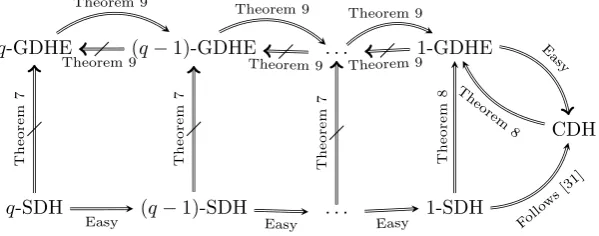
Having identified the q-GDHE and q-SFrac assumptions as being central for the security of target assumptions in general, we investigate their internal structure. We first show thatq-SFrac is unlikely to be able to serve as an Uber assumption on its own. More precisely, we show that for a generic group adver-sary the 2-GDHE assumption is not implied byq-SFrac assumptions. Second, we show that theq-GDHE assumptions appear to be strictly increasing asqgrows, i.e., if the (q+ 1)-GDHE holds, then so doesq-GDHE, but for a generic group adversary the (q+ 1)-GDHE may be false even thoughq-GDHE holds. We also analyze the particular case whereq= 1 and prove that the 1-GDHE assumption is equivalent to the CDH assumption. We summarize the implications we prove in Fig. 1, where A⇒Bdenotes thatBis implied (in a black-box manner) byA, whereasA=6⇒Bdenotes the absence of such an implication (cf. Section 2.1).

q-GDHE (q−1)-GDHE . . . 1-GDHE

CDH

q-SDH (q−1)-SDH . . . 1-SDH Theorem 9 _{Theorem 9}

Theorem 9

Theorem 9

Theorem 9

Easy Theorem 9

Theorem

8

Easy

Theorem

7

Theorem

7

Easy

Theorem

7

Easy

Theorem

8

Follo ws

[31]

Fig. 1: Summary of Reductions

Based on these results we view the q-GDHE and q-SFrac assumptions as a bulwark. Whatever type of target assumptions a cryptographer bases her schemes on, they are secure as long as neither the q-GDHE nor the q-SFrac assumptions are broken.3 _{Since the attacker has less leeway in the q-GDHE} as-sumptions, the cryptographer may choose to rely exclusively on target assumpi-tons that are implied by the q-GDHE assumptions, and we therefore identify a large class of target assumptions that only need theq-GDHE assumptions to hold.

We also have advice for the cryptanalyst. We believe it is better to focus on canary in a coal mine assumptions than the discrete logarithm problem that

3

has received the most attention so far. Based on our work, the easiest target assumptions to attack in single prime-order groups are theq-GDHE assumptions and the q-SFrac assumptions. The class of q-SFrac assumptions allows more room for the adversary to maneuver in the choice of polynomialsr(X) ands(X) and appears less structured than the q-GDHE assumptions. Pragmatically, we note that within the q-SFrac assumptions it is almost exclusively the q-SDH assumptions that are used. We therefore suggest theq-GDHE assumptions and theq-SDH assumptions to be the most suitable targets for cryptanalytic research. Switching from single prime-order groups_Gp to groups with a bilinear map

e:G1×G2→GT, a similar structure emerges. For target assumptions in the base

groupsG1andG2, we can again identify assumptions similar to theq-GDHE and q-SFrac assumptions that act as a joint Uber assumption. In the target groupGT,

a somewhat more complicated picture emerges under the influence of the pairing of source group elements. However, we can replace theq-GDHE assumption with an assumption we call the q-Bilinear Gap (q-BGap) assumption, and get that this assumption together with a natural generalization of theq-SFrac assumption to bilinear groups, which we name the q-BSFrac assumption, jointly act as an Uber assumption for all target assumptions in_GT.

A natural question is whether our analysis extends to other assumptions as well, for instance ”flexible” assumptions such as the q-HSDH assumption [12], where the adversary can choose secret exponents and therefore the target ele-ments are no longer uniquely determined. Usually assumptions in the literature involve group elements that have discrete logarithms defined by polynomials in secret values inZpchosen by a challenger and/or public values inZp. This gives

rise to several classes of assumptions:

1. Non-interactive assumptions where the advesary’s goal is to compute group elements defined by secret variables chosen by the challenger.

2. Non-interactive assumptions where the adversary’s goal is to compute group elements defined by secret variables chosen by the challenger and public values chosen by the adversary.

3. Non-interactive assumptions where the adversary’s goal is to compute group elements defined by secret variables chosen by the challenger, and public and secret values chosen by the adversary.

4. Interactive assumptions, where the challenger and adversary interact. Target assumptions include all assumptions in classes 1 and 2. However, class 3 includes assumptions which are not falsifiable, e.g. knowledge-of-exponent as-sumptions [5]. Since q-GDHE is in class 1 and q-SFrac is in class 2, both of which only have falsifiable assumptions, we cannot expect them to capture non-falsifiable assumptions in class 3. We leave it as an interesting open problem which structure, if any, can be found in classes 3 and 4, and we hope our work will inspire research on this question.

previous works such as [9, 11, 19, 34] which aimed at defining algebraic frame-works or templates in generic groups to capture some families of assumptions. The closest work to ours is Abdalla et al. [1], which provided an Uber assump-tion for decisional assumpassump-tions in cyclic groups (without a bilinear map, which invalidates many decisional assumptions). Other works, discussed above, have mostly dealt with specific relations among assumptions, e.g., the equivalence of CDH and square-CDH as opposed to the general approach we take.

Paper Organization. Our research contribution is organized into three parts. In Sec. 3, we define our framework for target assumptions in cyclic groups, and progressively seek reductions to simpler assumptions. In Sec. 4, we study the internal structure and the relationships among the families of assumptions we identify as Uber assumptions for our framework. In Sec. 5, we provide a generalization of our framework in the bilinear setting.

2

Preliminaries

Notation. We say a functionf isnegligiblewhenf(κ) =κ−ω(1) and it is over-whelming whenf(κ) = 1−κω(1). We writef(κ)≈0, when f(κ) is a negligible function. We will use κto denote a security parameter, with the intuition that asκgrows we expect stronger security.

We writey=A(x;r) when algorithmAon inputxand randomnessr, outputs y. We write y ←A(x) for the process of picking randomness rat random and setting y =A(x;r). We also write y ← S for sampling y uniformly at random from the set S. We will assume it is possible to sample uniformly at random from sets such as_Zp. We write PPT and DPT for probabilistic and deterministic

polynomial time respectively.

Quadratic Residuosity. For an odd primepand an integera6= 0, we sayais a

quadratic residue modulopif there exists a numberxsuch thatx2_{≡a(mod p)} and we say a is quadratic non-residue modulo potherwise. We denote the set of quadratic residues modulopby_QR(p) and the set of quadratic non-residues modulopby_QNR(p). By Euler’s theorem, we have|_QR(p)|=|_QNR(p)|=p−1₂ .

2.1 Non-interactive Assumptions

In a non-interactive computational problem the adversary is given a problem instance and tries to find a solution. We say the adversary breaks the problem if it has non-negligible chance of finding a valid solution and we say the problem is hard if any PPT adversary has negligible chance of breaking it. We focus on non-interactive problems that are efficiently falsifiable, i.e., given the instance there is an efficient verification algorithm that decides whether the adversary won.

(pub, priv)← I(1κ_{): I is a PPT algorithm that takes as input a security}

param-eter1κ, and outputs a pair of public/private information(pub, priv).

b← V(pub, priv, sol): V is a DPT algorithm that receives as input (pub, priv)

and a purported solutionsoland returns1 if it considers the answer correct and0otherwise.

The assumption is that for all PPT adversaries A, the advantageAdvA is

neg-ligible (inκ), where

AdvA(κ) := Pr [(pub, priv)← I(1κ);sol← A(pub) :V(pub, priv, sol) = 1].

Relations Among Assumptions. For two non-interactive assumptionsAand

B, we will use the notation A⇒B when assumption B is implied (in a black-box manner) by assumption A, i.e. given an efficient algorithmB for breaking assumptionB, one can construct an efficient algorithmAthat usesBas an oracle and breaks assumptionA. The absence of implication will be denoted byA=6⇒B.

2.2 Non-Interactive Assumptions over Cyclic Groups

We study non-interactive assumptions over prime-order cyclic groups. These assumptions are defined relative to a group generatorG.

Definition 2 (Group Generator).A group generator is a PPT algorithm G, which on input a security parameterκ(given in unary) outputs group parameters

(Gp, G), where

• _{Gp is cyclic group of known prime order pwith bitlength} |_p|_=Θ(κ). • _{Gp has a unique canonical representation of group elements, and polynomial}

time algorithms for carrying out group operations and deciding membership.

• _{Gis a uniformly random generator of the group.}

In non-interactive assumptions over prime-order groups the instance genera-tor runs the group setup (Gp, G)← G(1κ) and includesGp inpub. Sadeghi and

Steiner [38] distinguish between group setups with low, medium and high gran-ularity. In the low granularity setting the non-interactive assumption must hold with respect to random choices of_GpandG, in the medium granularity setting

it must hold for all choices of_Gp and a randomG, and in the high granularity

setting it must hold for all choices of _Gp and G. Our definitions always assume

Gis chosen uniformly at random, so depending on G we are always working in the low or medium granularity setting.

We will use [x] to denote the group element that has discrete logarithm x with respect to the group generator G. In this notation the group generatorG is [1] and the neutral element is [0]. We will find it convenient to use additive notation for the group operation, so we have [x] + [y] = [x+y]. Observe that givenα∈Zpand [x]∈Gpit is easy to compute [αx] using the group operations.

For a vector x = (x1, . . . , xn) ∈ Znp we use [x] as a shorthand for the tuple

([x1], . . . ,[xn])∈Gnp. We will occasionally abuse the notation and let [x1, . . . , xn]

There are many examples of non-interactive assumptions defined relative to a group generator G. We list in Fig. 2 some of the existing non-interactive computational assumptions.

Computational Diffie-Hellman (CDH) Assumption ICDH(1κ

)

(Gp,[1])← G(1κ);x, y←Zp

Return (pub= (Gp,[1],[x],[y]), priv= (x, y))

VCDH(pub, priv= (x, y), sol= [z]) If [z] = [xy] return 1

Else return 0

Square Computational Diffie-Hellman (SCDH) Assumption [32] ISCDH(1κ₎

(Gp,[1])← G(1κ);x←Zp

Return (pub= (Gp,[1],[x]), priv=x)

VSCDH(pub, priv=x, sol= [z]) If [z] =

x2

return 1 Else return 0

q-Generalized Diffie-Hellman Exponent (q-GDHE) Assumption [9, 10] Iq-GDHE(1κ)

(Gp,[1])← G(1κ);x←Zp

pub= (Gp,[1],[x], . . . ,xq−1,xq+1, . . . ,x2q) Return (pub, priv=x)

Vq-GDHE(pub, priv=x, sol= [z]) If [z] = [xq] return 1

Else return 0

q-Strong Diffie-Hellman (q-SDH) Assumption [8] Iq-SDH(1κ)

(Gp,[1])← G(1κ);x←Zp

Return (pub= (Gp,[1],[x], . . . ,[xq]), priv=x)

Vq-SDH(pub, priv=x, sol= (c,[z])) If [z] =h_x+1_ci&c∈Zp\ {−x} return 1 Else return 0

q-Diffie-Hellman Inversion (q-DHI) Assumption [33] Iq-DHI(1κ)

(Gp,[1])← G(1κ);x←Z×p

Return (pub= (Gp,[1],[x], . . . ,[xq]), priv=x)

Vq-DHI(pub, priv=x, sol= [z]) If [z] =1

x

return 1 Else return 0

Square Root Diffie-Hellman (SRDH) Assumption [29] ISRDH(1κ

)

(Gp,[1])← G(1κ);x←Zp Return pub= (Gp,[1],

x2), priv=x

VSRDH(pub, priv=x, sol= [z]) If [z] = [±x] return 1

Else return 0

Fig. 2: Some existing non-interactive intractability assumptions

Generic Group Model. Obviously, if an assumption can be broken using generic-group operations, then it is false. The absence of a generic-group attack on an assumption does not necessarily mean the assumption holds [18, 25] but is a necessary precondition for the assumption to be plausible.

We formalize the generic group model [36, 39] where an adversary can only use generic group operations as follows. GivenGpwe let [·] be a random bijection

Zp→Gp. We give oracle access to the addition operation, i.e.,O([x],[y]) returns

of deciding group membership. Also, given an arbitrary [x], she can compute [0] = [px] using the addition oracle. A generic adversary might be able to sample a random group element from Gp, but since they are just random encodings

we may without loss of generality assume she only generates elements as linear combinations of group elements she has already seen. All the assumptions listed in Fig. 2 are secure in the generic group model.

3

Target Assumptions

The assumptions that can be defined over cyclic groups are legion. We will focus on the broad class of non-interactive computational assumptions where the adversary’s goal is to compute a particular group element. We refer to them astarget assumptions.

The CDH assumption is an example of a target assumption where the ad-versary has to compute a specific group element. She is given ([1],[x],[y])∈G3p

and is tasked with computing [xy]∈Gp.

We aim for maximal generality of the class of assumptions and will therefore also capture assumptions where the adversary takes part in specifying the target element to be computed. In the q-SDH assumption for instance the adversary is given ([1],[x], . . . ,[xq])∈Gqp+1 and is tasked with finding c∈Zp and [_x+1_c]∈

Gp. Here the problem instance in itself does not dictate which group element

the adversary must compute but the output of the adversary includesc, which uniquely determines the target element to be computed.

We will now define target assumptions. The class will be defined very broadly in order to capture existing assumptions in the literature such as CDH and q-SDH as well as other assumptions that may appear in future works.

In a target assumption, the instance generator outputspub that includes a prime-order group, a number of group elements, and possibly some additional information. Often, the group elements are of the form [a(x)], where a is a polynomial andxis chosen uniformly at random fromZp. We generalize this by

letting the instance generator output group elements of the form [a_b((x_x)₎], where a(X) and b(X) are multi-variate polynomials and x is chosen uniformly at random from_Zm

p . We will assume all the polynomials are known to the adversary,

i.e., they will be explicitly given in the additional information inpubin the form of their coefficients. The adversary will now specify a target group element. She does so by specifying polynomials r(X) and s(X) and making an attempt at computing the group element [r_s(₍x_x))].

If the target element can be computed using generic-group operations on the group elements in pub, then the problem is easy to solve and hence the assumption is trivially false. To exclude trivially false assumptions, the solution verifier will therefore check that for all fixed linear combinationsα1, . . . , αn∈Zp

there is a low probability over the choice of x that r_s(₍x_x)₎ = P

iαia_bi(x)

i(x). The

Definition 3 (Target Assumption). Given polynomialsd(κ), m(κ)andn(κ)

we say (I,V)is a (d, m, n)-target assumption for G if they can be defined by a PPT algorithmIcore _{and a DPT algorithmV}core _{such that}

(pub, priv)← I(1κ): AlgorithmI proceeds as follows:

• _(Gp,[1])← G₍₁κ₎ •

n_a

i(X)

bi(X)

on

i=1

, pub0, priv0← Icore₍ Gp)

• _x←_Zm

p conditioned onbi(x)6= 0

• _pub:=

Gp,

nh_a

i(x)

bi(x)

ion

i=1, n_a

i(X)

bi(X)

on

i=1, pub 0

• _{Return(pub, priv= ([1],x, priv}0₎₎

0/1← V pub, priv, sol= r(X), s(X),[y], sol0: AlgorithmVreturns1if all of the following checks pass and0 otherwise:

• _r(X)Qn

i=1bi(X)∈/ span

n

s(X)aj(X)Qi6=jbi(X)

on

j=1

• _{[y] =} r(x)

s(x)[1]

• Vcore_{(pub, priv, sol) = 1}

We require that the number of indeterminates inXism(κ)and each of the poly-nomialsa1(X), b1(X), . . . , an(X), bn(X), r(X), s(X)has a total degree bounded

by d(κ), both of which can easily be checked byVcore_.

It is easy to see that all assumptions in Fig. 2 are target assumptions. For CDH for instance, we have d= 2, m= 2, n= 3, a1(X1, X2) = 1, a2(X1, X2) = X1, a3(X1, X2) = X2, and b1(X1, X2) = b2(X1, X2) = b3(X1, X2) = 1. Al-gorithm Vcore _{then checks that the adversary’s output is r(X1, X2) = X1X2} and s(X1, X2) = 1, which means the adverary is trying to compute the target [x1x2]∈Gp.

Inq-SDH we have d=q,m= 1, n=q+ 1,ai(X) =Xi−1, andbi(X) = 1

for i = 1, . . . , q+ 1. AlgorithmVcore _{checks that the target polynomials are of} the formr(X) = 1 ands(X) = c+X for somec∈Zp, meaning the adversary

it is trying to compute the target [_x+1_c]∈Gp.

3.1 Simple Target Assumptions

We now have a very general definition of target assumptions relating to the computation of group elements. In the following subsections, we go through progressively simpler classes of assumptions that imply the security of target assumptions. We start by defining simple target assumptions, where the divisor polynomials in the instance are trivial, i.e.,b1(X) =· · ·=bn(X) = 1.

Definition 4 (Simple Target Assumption). We say a (d, m, n)-target as-sumption(I,V)forGis simple if the instance generator always picks polynomials

AlgorithmIB(1κ) - (_Gp,[1])← G(1κ)

- nai(X)

bi(X)

on

i=1, pub 0 A, priv0A

← Icore A (Gp)

- Fori= 1, . . . , nsetci(X) :=aiQj6=ibj(X)

-x←Zmp

-pub_B= _Gp,{[ci(x)]}n_i=1,{ci(X)}n_i=1, pub0B = {ai(X), bi(X)}ni=1, pub 0 A

- Return (pub_B, priv_B = ([1],x, priv0_A))

AlgorithmVB pubB, privB= ([1],x, priv 0

A), solB = t(X), s(X),[y], sol 0

- Checkt(X)∈/ span{s(X)c1(X), . . . , s(X)cn(X)}

- Check [y] = _st(₍x_x)₎[1] - Checkt(X) =r(X)Qn

j=1bj(X) for a polynomialr(X) of total degree≤d

- Letpub_A= (_Gp,{[ci(x)]}n_i=1,

n_a

i(X)

bi(X)

on

i=1 , pub0_A) - Letpriv_A= ([Qn

j=1bj(x)],x, priv0A) - CheckVcore

A pubA, privA, solA = (r(X), s(X),[y], sol0)

= 1 AdversaryB Gp,{[ci(x)]}

n

i=1,{ci(X)} n

i=1,{ai(X), bi(X)} n i=1, pub

0 A

- r(X), s(X),[y], sol0← AGp,{[ci(x)]} n i=1,

n_a

i(X)

bi(X)

on

i=1, pub 0 A

- ReturnsolB =

t(X) =r(X)Qn

j=1bj(X), s(X),[y], sol0

Fig. 3: Simple target assumptionB= (IB,VB) and adversaryB against it

Next, we will prove that the security of simple target assumptions implies the security of all target assumptions. The idea is to reinterpret the tuple the adversary gets using the random generator [1] to having random generator [Qn

i=1bi(x)]. Now all fractions of formal polynomials are scaled up by a

fac-torQn

i=1bi(X) and the divisor polynomials can be cancelled out.

Theorem 1. For any (d, m, n)-target assumption A = (IA,VA) there exists a ((n+ 1)d, m, n)-simple target assumption B= (IB,VB)such that B⇒A.

Proof. Given an assumption A = (IA,VA) and an adversary A against it, we define a simple target assumption B= (IB,VB) and an adversaryB (that uses adversaryAin a black-box manner) against it as illustrated in Fig. 3. The key observation is that as long asQn

i=1bi(x)6= 0, the two vectors of group elements

([c1(x)], . . . ,[cn(x)]) and

[a1(x)

b1(x)], . . . ,[

an(x)

bn(x)]

are identically distributed. By the specification of assumption A, it follows that bi(X)6≡ 0 for all i∈ {1, . . . , n}.

By the Schwartz-Zippel lemma, the probability that Qn

i=1bi(x) = 0 is at most dn

p. Thus, ifA has success probabilityA, then Bhas success probabilityB≥

A−dn

3.2 Univariate Target Assumptions imply Multivariate Target Assumptions

We will now show that security of target assumptions involving univariate poly-nomials imply security of target assumptions involving multivariate polypoly-nomials.

Theorem 2. For any (d, m, n)-simple target assumption A = (IA,VA) there

exists a((n+ 1)d,1, n)-simple target assumptionB= (IB,VB)where B⇒A. Proof. Given A = (IA,VA) and an adversary A with success probability A against it, we define a simple target assumption (IB,VB) with univariate poly-nomials and construct an adversary B (that uses A in a black-box manner) against it as illustrated in Fig. 4.

AlgorithmI_B(1κ₎

- (_Gp,[1])← G(1κ)

-{ai(X)}n_i=1, pub0A, priv 0 A

← Icore A (Gp)

- Randomly choose c(X)←(_Zp[X])m where deg(ci) =n+ 1

- Fori= 1, . . . , nletbi(X) :=ai(c(X))

-pub0_B:= {ai(X)}ni=1,c(X), pub 0 A

-x←_Zp

- Return pub_B= _Gp,{[bi(x)]} n

i=1,{bi(X)}ni=1, pub 0 B

, priv_B= ([1], x, priv0_A) AlgorithmVB pubB, privB, solB= r(X), s(X),[y],(rA(X), sA(X), sol0A)

- Checkr(X)∈/ span{s(X)b1(X), . . . , s(X)bn(X)}

- Check [y] = r_s(_(xx)₎[1]

- Letpub_A= (Gp,{[bi(x)]}in=1,{ai(X)}ni=1, pub 0 A) - Letpriv_A= ([1], x, priv0_A)

- CheckVcore

A pubA, privA, solA = (rA(X), sA(X),[y], sol 0 A)

= 1 AdversaryB Gp,{[bi(x)]}n_i=1,{bi(X)}n_i=1, pub0B

- rA(X), sA(X),[y], sol0_A

← A Gp,{[bi(x)]} n

i=1,{ai(X)} n i=1, pub

0 A

- Return rA(c(X)), sA(c(X)),[y], sol_B0 = (rA(X), sA(X), sol0_A)

Fig. 4: Univariate simple target assumptionBand adversaryBagainst it

Without loss of generality we can assumea1(X), . . . , an(X) are linearly

inde-pendent, and therefore the polynomialsrA(X) andsA(X)a1(X), . . . , sA(X)an(X)

infor-mation aboutc(X) thatBpasses on toAcan be computed from (x,c(x)). This meansBhas advantageB≥A−d(np+1) against assumptionB.

u t

Lemma 1. Let a1(X), . . . , an(X) ∈ Zp[X] be linearly independent m-variate

polynomials of total degree bounded byd, and let (x,x)∈Zp×Zmp. Pick a vector

of m random univariate degree n polynomials c(X) ∈ (_Zp[X]) m

that passes through (x,x), i.e., c(x) = x. The probability that a1(c(X)), . . . , an(c(X)) are

linearly independent is at least1−dn p.

Proof. Takenrandom pointsx1, . . . ,xn ∈Zmp and consider the matrix

M =   

a1(x1)· · ·a1(xn)

..

. ...

an(x1)· · ·an(xn)

  .

We will argue by induction that with probability 1−dn

p the matrix is

invert-ible. Forn= 1 it follows from the Schwartz-Zippel lemma that the probability a1(x1) = 0 is at mostd_p. Suppose now by induction hypothesis that we have prob-ability 1−d(n_p−1)that the top left (n−1)×(n−1) matrix is invertible. When it is invertible, the valuesan(x1), . . . , an(xn−1) uniquely determineα1, . . . , αn−1such that forj= 1, . . . , n−1 we havean(xj) =P

n−1

i=1 αiai(xj). Since the

polynomi-alsa1(X), . . . , an(X) are linearly independent, by the Schwartz-Zippel lemma,

there is at most probability d_pthat we also havean(xn) =P n−1

i=1 αiai(xn). So the

row (an(x1), . . . , an(xn)) is linearly independent of the other rows, and hence

we have M is invertible with at least probability 1−d(n_p−1)−d p = 1−

dn p .

Finally, picking a vector of m random polynomials c(X) of degree n such that c(x) =x and evaluating it in distinct pointsx1, . . . , xn ←Zp\ {x} gives

usnrandom pointsc(xj)∈Zmp . So the matrix

  

a1(c(x1))· · ·a1(c(xn))

..

. ...

an(c(x1))· · ·an(c(xn))

  

has at least probability 1−dn

p of being invertible. If

Pn

i=1αiai(c(X)) = 0, then

it must hold in the distinct points x1, . . . , xn, and we can see there is only the

trivial linear combination withα1=· · ·=αn = 0. ut

3.3 Polynomial Assumptions

We now consider simple target assumptions with univariate polynomials where s(X) is fixed. We can without loss of generality assume this meanspriv0 output by the instance generator containss(X) and the solution verifier checks whether the adversary’s solution matchess(X). There are many assumptions wheres(X) is fixed, in the Diffie-Hellman inversion assumption we will for instance always haves(X) =Xand in theq-GDHE assumption we always haves(X) = 1. When the polynomials(X) is fixed, we can multiply it away as we did for the multivari-ate polynomials b1(X), . . . , bn(X) when reducing target assumptions to simple

target assumptions. This leads us to define the following class of assumptions:

Definition 5 (Polynomial Assumption). We say a (d,1, n)-simple target assumption (I,V) forG is a (d, n)-polynomial assumption if V only accepts a solution withs(X) = 1.

We leave the proof of the following theorem to the reader.

Theorem 3. For any (d,1, n)-simple target assumption A = (IA,VA) for G

where the polynomial s(X) is fixed, there is a (2d, n)-polynomial assumption B= (IB,VB)whereB⇒A.

We will now show that all polynomial assumptions are implied by the gen-eralized Diffie-Hellman exponent (q-GDHE) assumptions (cf. Fig. 2) along the lines of [22]. This means the q-GDHE assumptions are Uber assumptions that imply the security of a major class of target assumptions, which includes a ma-jority of the non-interactive computational assumptions for prime-order groups found in the literature.

Theorem 4. For any(d, n)-polynomial assumptionA= (IA,VA)forG we have that (d+ 1)-GDHE⇒A.

Proof. LetAbe an adversary against the (d, n)-polynomial assumption. We show how to build an adversaryB, which usesAin a black-box manner to break the (d+1)-GDHE assumption. AdversaryBgets [1],[x], . . . ,

xd

,[xd+2_{], . . . ,} x2d+2 from the (d+ 1)-GDHE instance generator and her aim is to output the element

xd+1

∈_Gp. AdversaryB uses algorithmI_Acore to generate a simulated

polyno-mial problem instance as described below, which she then forwards toA. AdversaryB Gp,[1],[x], . . . ,

xd,xd+2, . . . ,x2d+2 - {ai(X)}

n i=1, pub

0 A, priv0A

← Icore A (Gp)

- Randomly choose c(X)←Zp[X] where deg(c) =d+ 1 and

noai(X)c(X) includes the termXd+1

- For allicompute [ai(x)c(x)] using the (d+ 1)-GDHE tuple

- Run (r(X),[y], sol0)← A Gp,{[ai(x)c(x)]}ni=1,{ai(X)} n i=1, pub

0 A

- Parser(X)c(X) as P2_i=0d+1tiXi

- Return _t1

d+1

[y]−[P

i6=d+1tixi]

Assuming c(x) 6= 0, which happens with probability 1− d+1

p , the input to A

looks identical to a normal problem instance for assumption Awith generator [c(x)]. Furthermore, if Afinds a satisfactory solution to this problem, we then have [y] =r(x)[c(x)]. By Lemma 2 below there is at most 1_p chance of returning r(X) such thatr(X)c(X) has coefficient 0 forXd+1_{and hence using the (2d+ 2)} elements from the (d+ 1)-GDHE tuple, we can recover [xd+1_{] from [y]. We now} get that ifAhas advantageAagainstA, then Bhas advantageB≥A−d+2p

against the (d+ 1)-GDHE assumption. ut

Lemma 2 (Lemma 10 from [22]). Let {ai(X)}n_i=1 be polynomials of

de-gree at most d. Pick x ← Zp and c(X) as a random degree d+ 1 polynomial

such that all products bi(X) = ai(X)c(X) have coefficient 0 for Xd+1. Given

({ai(X)} n

i=1, x, c(x)), the probability of guessing a non-trivial degree d

polyno-mial r(X)such that r(X)c(X)has coefficient 0 forXd+1 is at most 1_p.

3.4 Fractional Assumptions

We now consider the alternative case of simple target assumptions with uni-variate polynomials, wheres(X) is not fixed. Whens(X)|r(X), we can without loss of generality divide out and get s(X) = 1. The remaining case is when s(X)-r(X), which we now treat.

Definition 6 ((d, n)-Fractional Assumption).We say a(d,1, n)-simple tar-get assumption (I,V)forG is an (d, n)-fractional assumption ifV only accepts the solution ifs(X)-r(X).

Next we define a simple fractional assumption which we refer to for short as q-SFrac, which says given the tuple ([1],[x],[x2], . . . ,[xq]) it is hard to compute h_r(x)

s(x) i

when deg(r)<deg(s). The simple fractional assumption is a straightfor-ward generalization of theq-SDH assumption, where deg(r) = 0 sincer(X) = 1 and deg(s) = 1. A proof for the intractability of theq-SFrac assumption in the generic group model can be found in the full version [23].

Definition 7 (q-SFrac Assumption). The q-SFrac assumption is a simple target assumption wheren=q+ 1,ai(X) =Xi−1, and0≤deg(r)<deg(s)≤q.

We now prove the following theorem.

Theorem 5. For any (d, n)-fractional assumption A = (I,V) for G we have

d-SFrac⇒A.

Proof. LetAbe an adversary against a (d, n)-fractional assumptionA. We show how to use A to construct an adversary B against the d-SFrac assumption. Adversary B gets _Gp,[1],[x], . . . ,

xd

from her environment and her aim is to output a valid solution of the form r0(X), s0(X),h_sr00(₍x_x)₎

i

fractional assumption as described below to generate a problem instance, which she then forwards toA.

AlgorithmB(_Gp,[1],[x], . . . ,[xd])

- {ai(X)} n i=1, pub

0_{, priv}0

← Icore₍ Gp)

- For allicompute [ai(x)] using thed-SFrac tuple [1] [x], . . . ,

xd - Run (r(X), s(X),[y])← A Gp,{[ai(x)]}

n

i=1,{ai(X)} n i=1, pub

0

- Letr0_{(X) =r(X) mods(X) and writer(X) =t(X)s(X) +r}0_(X) - Use the tuple [1],[x], . . . ,xdto computet(x)

- Return (r(X)0_{, s(X),[y]−[t(x)])}

The advantage of adversary B against the d-SFrac assumption is the same as that of adversaryAagainst the fractional assumptionA. ut

3.5 The q-SFrac and q-GDHE Assumptions Together Imply All Target Assumptions in Cyclic Groups

We now prove that the q-SFrac andq-GDHE assumptions together constitute an Uber assumption for all target assumptions in prime-order cyclic groups.

Theorem 6. There is a polynomial q(d, m, n) such that the joint q-SFrac and

q-GDHE assumption implies all(d, m, n)-target assumptions.

Proof. LetAbe a (d, m, n)-target assumption. By Theorem 1, for any adversary A with advantage A against A, we can define a (d(n+ 1), m, n)-simple target assumption A1 and an adversaryA1 with advantage A₁ ≥A−

dn

p against it.

By Theorem 2, using A1 against A1, we can define a (d(n+ 1)2,1, n)-simple target assumption A2 and an adversary A2 against it with advantage A₂ ≥ A₁−

d(n+1)2

p ≥A−

d(n+(n+1)2₎

p . We now have two cases as follows:

• _{With non-negligible probability a successful solution hassA}

2(X) - rA2(X). By Theorem 5, we can use A2 to construct an adversary A3 against the (d(n+1)2_{)-SFrac assumption where advantage}

A₃ ≥A₂ ≥A−

d(n+(n+1)2)

p .

Since by defintiond, n∈Poly(κ) and logp∈θ(κ), it follows that d(n+(n_p+1)2) is negligible (inκ).

• _{With overwhelming probability a successful solution uses polynomials where} sA₂(X)|rA₂(X) which is equivalent to the case wheresA₂(X) = 1. By Theo-rem 3, usingA2we can define a (2d(n+1)2, n)-polynomial assumptionA3and an adversaryA3 with advantageA₃ ≥A₂−

4d(n+1)2

p ≥A−

d(n+5(n+1)2₎

p .

By Theorem 4, using adversary A3, we can construct an adversary A4 against the (2d(n+ 1)2_{+ 1)-GDHE assumption with advantage}

A₄ ≥A₃− 2d(n+1)2₊₂

p . From which it follows thatA₄ ≥A−

d(7(n+1)2_+n)+2

p . Since by

defintion d, n ∈ Poly(κ) and logp ∈ θ(κ), it follows that d(7(n+1)_p2+n)+2 is negligible (inκ).

4

The Relationship between the GDHE and SFrac

Assumptions

Having identified the q-GDHE and q-SFrac assumptions as Uber assumptions for all target assumptions, it is natural to investigate their internal structure and their relationship to each other. One obvious question is whether a further simplification is possible and one of the assumption classes imply the other. We first analyze the case whereq≥2 and show thatq-SFrac does not imply 2-GDHE for generic algorithms. This means that we need the q-GDHE assumptions to capture the polynomial target assumptions, theq-SFrac assumptions cannot act as an Uber assumption for all target assumptions on their own.

We also look at the lowest level of theq-SFrac andq-GDHE hierarchies. Ob-serve that the 1-SFrac assumption is equivalent to the 1-SDH assumption. We prove that the 1-GDHE assumption is equivalent to the CDH assumption. This immediately also gives us that the 1-SFrac assumption implies the 1-GDHE as-sumption since the 1-SDH asas-sumption implies the CDH asas-sumption. A summary of the implications we prove can be found in Fig. 1.

4.1 The SFrac Assumptions Do Not Imply the 2-GDHE Assumption

We prove here that the i-GDHE assumption for i ≥ 2 is not implied by any q-SFrac assumption for generic adversaries, i.e. q-SFrac

GGM

6

=⇒i-GDHE for alli ≥ 2. More precisely, we show that providing an unbounded generic adversary A against a q-SFrac assumption with a 2-GDHE oracle O2-GDHE, which on input

([a],[b],[c],[d]) where b=az,c=az3_,d=az4 _{returns the element} az2

, and returns the symbol⊥if the input is malformed, does not help the adversary.

Theorem 7. The q-SFrac assumption does not imply the2-GDHE assumption in generic groups.

Proof. Consider a generic adversaryA which gets input ([1],[x], . . . ,[xq_{]) and}

is tasked with outputting _sr(_(XX)₎,hr_s((_xx)₎i, where 0≤deg(r)< deg(s) ≤q. We giveAaccess to an oracleO_2-GDHE(·,·,·,·) as above, which can be queried poly-nomially many times.

Since A is generic, the tuple ([a],[b],[c],[d]) she uses as input in her 1-st O_2-GDHE query can only be linear combinations of the elements [1],[x], . . . ,[xq_].

Thus, we have

a=

q

X

j=0

αjxj b= q

X

j=0

βjxj c= q

X

j=0 γjxj

for known αj, βj, γj. Let the corresponding formal polynomials be a(X), b(X)

andc(X), respectively. We have that deg(a),deg(b),deg(c)∈ {0, . . . , q}. By def-inition, for the input to the oracle O2-GDHE to be well-formed, we must have

probability of holding unlesszcorresponds to some (possibly rational) function z(X) and we have b(X) =a(X)z(X) and c(X) =a(X)z(X)3 when viewed as formal polynomials.

If the adversary submits a query wherea(X)≡0 orb(X)≡0, the oracle will just return [0], which is useless to the adversary. So from now on let’s assume that a(X)6≡0,b(X)6≡0 andc(X)6≡0.

We now have

c(X) =a(X)z(X)3=a(X) _b(X)

a(X) 3

= b(X) 3

a(X)2.

This means a(X)2_|b(X)3_{, which implies a(X)|b(X)}2_{. The answer returned by} the oracle on a well-formed input corresponds toa(X)z(X)2_=a(X)b(X)

a(X) 2

=

b(X)2

a(X). Sincea(X)|b(X)

2_{, the answer corresponds to a proper polynomial.} If deg(b)≤deg(a), we have 2 deg(b)−deg(a)≤deg(b)≤q, and if deg(b)≥ deg(a), we have 2 deg(b)−deg(a) ≤ 3 deg(b)−2 deg(a) = deg(c) ≤ q. Thus, the answer the oracle returns corresponds to a known polynomial of degree in {0, . . . , q}which could have been computed by the adversary herself using generic group operations on the tuple [1],[x], . . . ,[xq_{] without calling the oracle. ut}

Since as we prove later the GDHE assumptions family is strictly increasingly stronger, we get the following corollary.

Corollary 1. For all i≥2 it holds thatq-SFrac

GGM

6

=⇒i-GDHE.

4.2 CDH Implies the 1-GDHE Assumption

Since having access to a CDH oracle allows one to compute any polynomial in the exponent [31] (in fact, such an oracle provides more power as it allows computing even rational functions in the exponent for groups with known order [31]), it is clear that 1-GDHE⇒CDH andq-SDH⇒CDH. We prove in this section the implication CDH⇒1-GDHE, which means that the assumptions CDH and 1-GDHE are equivalent. As a corollaryq-SFrac⇒1-GDHE for allq.

We start by proving that the square computational Diffie-Hellman assump-tion (SCDH) (cf. Fig. 2), which is equivalent to the CDH assumpassump-tion [3, 26], implies the square root Diffie-Hellman (SRDH) assumption [29] (cf. Fig. 2) 4_. Note that given a SCDH oracle, one can solve any CDH instance by making 2 calls to the SCDH oracle. Let ([1],[a],[b]) ∈ G3p be a CDH instance, we have

[ab] =1₄([(a+b)2]−([(a−b)2])).

We remark here that Roh and Hahn [37] also gave a reduction from the SCDH assumption to the SRDH assumption. However, their reduction relies on two assumptions: that the oracle will always (i.e. with probability 1) return a

4

correct answer when queried on quadratic-residue elements and uniformly ran-dom elements when queried on quadratic non-residue elements, and that the prime order of the groupphas the special formp= 2tq+ 1 where 2t=O(κO(1)). Our reduction is more general since we do not place any restrictions on t or q and more efficient since it uses 4t+ 2|q|oracle queries, whereas their reduction uses O(t(2t_{+|q|)) oracle queries. Later on, we will also show how to boost an}

imperfect 1-GDHE oracle to get a SCDH oracle.

The Perfect Oracle Case. We prove that a perfect SRDH oracleOSRDHwhich on input a pair ([a],[az])∈G2p returns the symbol QNR (which for convenience

we denote by [0]) if z /∈ QR(p) and [±a √

z] otherwise, leads to a break of the SCDH assumption. The role of the exponentais to allow queries on pairs w.r.t. a different group generator than the default one. Letp= 2t_{q+1 for an odd positive}

integerqbe the prime order of the group_Gp. Note that whenp≡3 (mod 4) (this

is the case when−1∈_QNR(p)), we havet= 1, and in the special case wherep is a safe prime,qis also a prime. On the other hand, whenp≡1 (mod 4) (this is the case when −1∈_QR(p)), we havet >1.

In the following letω ∈ QNR(p) be an arbitrary 2t-th root of unity of Z×p,

i.e., ω2t−1 _{≡ −1 mod (p−1) and ω}2t _{≡ 1 mod (p−1). Note that there are} φ(2t_{) = 2}t−1 _{roots of unity and finding one is easy since for any generatorg of} Z×p, gq is a 2t-th root of unity. Observe that all elements in Z×p can be written

in the form ωiβ, where β has odd orderk|q. The quadratic residues are those whereiis even, and the quadratic non-residues are the ones whereiis odd.

Theorem 8. Given a perfect OSRDH oracle, we can solve any SCDH instance using at most4t+ 2|q|oracle calls when the group order is p= 2t_{q+ 1 for odd}

q.

Proof. Given a SCDH instance ([1],[x])∈G2p, our task is to compute

x2

∈Gp.

The task is trivial when x= 0, so let’s from now on assume x6= 0. Since any x∈_Z×

p can be written as x=ωiβ whereω ∈Z×p is a 2t-th root of unity and

β ∈_Z×

p has an odd orderkwherek|q, our task is to compute

x2

= ω2i_β2

. In the following, we will first describe an algorithmFindExpithat uses the square-root oracle to determinei. Next, we describe an algorithmSquarethat computes [y] =

ωj_β2

for some j, and then use FindExpi to clean it up to get x2

=

ω2i−j_{y] = [ω}2i_β2

. Both of these algorithms are given in Fig. 5.

Recall the perfect SRDH oracle responds with QNR, i.e. [0], whenever it gets a quadratic non-residue as input, i.e., whenever it gets input ([1],[ωi_{β]) for an}

odd i and β has an odd order. When it gets a quadratic residue as input, i.e., when i is even, it returns h±ω2iβ12

i

. Since ω2t−1 = −1 this means it returns either hω2iβ

1 2

i

orhω2t−1+i

2β 1 2

i .

Let the binary expansion of the exponent be i = it−1it−2. . . i0. In the

1 Algorithm FindExpi([1],[x], ω) 2 [y]←[x]

3 i←0

4 For j= 0 to t−1 : 5 [z]← OSRDH([1],[y])

6 If [z] = [0] /* QNR */ 7 i←i+ 2j

8 [y]← O_SRDH([1],[ω−1y]) 9 Else

10 [y]←[z] 11 Return i

1 Algorithm Square([1],[x], ω) 2 [y]← OSRDH([1],[x])

3 If [y] = [0] /* QNR */ 4 [y]← O_SRDH([1],[ωy]) 5 h←q+1

2

6 While h >2 : 7 If h is even 8 [z]← O_SRDH([1],[y])

9 If [z] = [0] /* QNR */

10 [y]← O_SRDH([1],[ωy])

11 Else

12 [y]←[z] 13 h← h₂

14 Else /* h is odd */ 15 [z]← O_SRDH([x],[y])

16 If [z] = [0] /* QNR */

17 [y]← O_SRDH([x],[ωy])

18 Else

19 [y]←[z] 20 h← h+1₂ 21 i←FindExpi([1],[x], ω) 22 j←FindExpi([1],[y], ω) 23 Return [ω2i−jy]

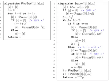
Fig. 5: Algorithms FindExpiandSquare used in the proof of Theorem 8

element with exponent itit−1. . . i1 on the second input. Which call returns a non-trivial group element tells us what i0 is and in both cases we get a new element where the bits have been shifted right and a new most significant bitit

has been added. Repeatingt times allows us to learn all ofi=it−1. . . i0. Next we describe the Square algorithm. The idea behind this algorithm is that given [ωi_{β] we want to compute [ω}j_β2_{] for some j, but we do not care} much about the root of unity part, i.e., whatjis, since we can always determine that by calling FindExpiand clean it up later. As a first step one of the inputs ([1],[x]) or ([1],[ωx]) will correspond to a quadratic residue and the square root oracle will return some [y] = [ωj_β1

2] = [ωjβ

q+1

2 ]. Let’s defineh= q+1

2 , which is a positive integer, so we have [y] = [ωj_βh_].

The idea now is that we will use repeated applications of the SRDH oracle to halvehuntil we get down toh= 2. Ifhis even, this works fine as one of the pairs ([1],[ωjβh]) or ([1],[ωj+1βh]) will correspond to a quadratic residue and we get a new element of the form [ωj0_βh0_{], whereh}0₌ h

2.

Repeated application of these two types of calls, depending on whetherhis even or odd, eventually gives us an element of the form [ωjβ2]. At this stage, we can use theFindExpialgorithm to determineiandj, which makes it easy to compute [x2] =ω2i−j[ωjβ2].

We now analyse the time complexity of the algorithms. AlgorithmFindExpi

makes at most 2t oracle calls, whereas Square makes at most 2|q| oracle calls plus two invocations ofFindExpi, i.e., at most 4t+ 2|q|oracle calls in total. ut

Using an Adversarial O∗

1-GDHE Oracle. In Theorem 8, we assumed the

re-duction had a perfectOSRDHoracle. Here we weaken the assumption used in the reduction and consider anO∗

1-GDHE oracle that returns a correct answer with a non-negligible probabilitywhen queried on a quadratic residue element. More precisely, let ([a],[b])∈G2pbe the input we are about to query theO∗1-GDHE ora-cle on. Since we can easily detect ifb= 0, we can assume that we never need to query to oracle on any input whereb= 0. When queried on ([a],[b])∈G×p ×G×p,

the oracle will return either the symbol QNR, i.e. [0]∈Gp or [c]∈Gp for some

c∈Z×p. Our assumption about correctness is

Prh(_Gp,[1])← G(1κ);a, z←Z×p :O∗1-GDHE([a],[az

2_{]) =±[az]}i_≥(κ). The oracle can behave arbitrarily when it does not return a correct answer or when the input is not a quadratic residue.

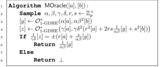
We will now show that we can rectify the adversarial behaviour of the oracle so that it cannot adapt its answer based on the instance input. The idea is to randomize the inputs to be queried to the oracle so that they are uniformly dis-tributed over the input space and we getchance of getting a correct square-root when the input is a quadratic residue. To check the solution, we then randomize an element related to the answer, which we can use to detect when the ora-cle is misbehaving. The result is a Monte Carlo algorithm described in Fig. 6, which with probability0 _≥2 _{returns a correct square-root when queried on a} quadratic residue and⊥in all other cases.

1 Algorithm MOracle([a],[b]) :

2 Sample α, β, γ, δ, r, s←_Z×_p

3 [y]← O_1-GDHE∗ (α[a], αβ2[b])

4 [z]← O∗_1-GDHE γ[a], γδ2(r2[a] + 2rs 1

αβ[y] +s

2_[b])

5 If _γδ1[z] =±(r[a] +_αβs [y])

6 Return _αβ1 [y]

7 Else

8 Return ⊥

Lemma 3. Using O∗

1-GDHE which returns a correct answer with probability ,

algorithmMOraclereturns a correct answer with probability0≥2when queried on a well-formed pair ([a],[b])∈G×p ×G×p and⊥otherwise.

Proof. If b

a ∈ QR(p), we also have β2b

a ∈ QR(p), and when b

a ∈/ QR(p), we

also have β_a2b ∈/ _QR(p). We have probability that the answer [y] is a correct answer when b

a ∈ QR(p) in which case y = ±αβa

q

b

a, we can thus recover

[±aqb a =±

√

ab] by computing 1

αβ[y]. Lety

0₌ y αβ =±

√

ab. We have probability

that [z] is a correct answer. Now letz0= _γδz.

Note thatr2_{a+ 2rsy}0_+s2_{b= (ra+sy}0₎2_+s2_(b−y02_{) and if [z] is a correct} answer then we have z0 = ±(ra+sy0). Thus, we have probability at least 2 that algorithmMOraclewill return a correct square root when the input is well-formed.

We now argue that ify0 6=±√ab, with overwhelming probability the algo-rithm will return⊥. Letτ =a(r2a+ 2rsy0+s2b) =r2a2+ 2arsy0+s2ab.

Sincea(r2a+ 2rsy0+s2b) = (ra+sy0)2+s2(ab−y02), the query to the oracle is determined bya andτ, and there are roughlyp2 _{pairs (r, s) mapping into a} maximum ofpchoices ofτ. Therefore, for the same oracle query there are many possible valuesscould have. Now ify0 6=±√ab, i.e.yis an incorrect answer, then the oracle has negligible chance of passing the testz0 =±(ra+sy0) in line 5. If the test passes, thenz02= (ra+sy0)2_=r2_a2_{+ 2arsy}0_+s2_ab=τ−s2_(ab−y02_). Sincesis information-theoretically undetermined fromaandτ, there is negligible chance over the choice ofsthat this equality holds unlessab−y02= 0. ut Since is non-negligible, there must be a constant c > 0 such that for in-finitely many κ we have 0 _≥κ−c_{. We can use repetitions to boost the oracle}

to give the correct answer with overwhelming probability on theseκvalues, i.e., on quadratic residues it returns square-roots and on quadratic non-residues it returns⊥ or equivalently [0]. Chernoff-bounds ensure we only need κ

2

polyno-mially iterations of the Monte Carlo algorithm to build a good SRDH oracle.

4.3 The q-GDHE Family Structure

We say a family of assumptions {q-A} is a strictly increasingly stronger family if for all polynomials q≤q0 it holds that q0-A⇒q-Abutq-A=6⇒(q0+ 1)-A.

A proof for the following theorem can be found in the full version [23].

Theorem 9. The q-GDHE family is a strictly increasingly stronger family.

5

Target Assumptions over Bilinear Groups

specific group element in the base groups or the target group. For instance, the bilinear variants of the matrix computational Diffie-Hellman assumption in [34] (which implies the (computational bilinear)k-linear assumptions), the (bilinear) q-SDH assumptions, and the bilinear assumptions studied in [26] are all examples of target assumptions in bilinear groups.

Definition 8 (Bilinear Group Generator). A bilinear group generator is a PPT algorithm BG, which on input a security parameter κ (given in unary) outputs bilinear group parameters (G1,G2,GT, G1, G2), where

• _{G1,G2,GT are cyclic groups of prime orderpwith bitlength} |_p|_=Θ(κ). • _G1,_G2,_GT have polynomial-time algorithms for carrying out group

opera-tions and unique representaopera-tions for group elements.

• _{There is an efficiently computable bilinear map (pairing)e:G1}×_G2→_GT. • _{G1andG2are independently chosen uniformly random generators ofG1and}

G2, respectively, and e(G1, G2)generatesGT.

Again, we will be working in the low/medium granularity setting so we always assume uniformly random generators of the base groups.

According to [21], bilinear groups of prime order can be classified into 3 main types depending on the existence of efficiently computable isomorphisms between the groups. In Type-1, G1 =G2. In Type-2 G1 6= G2 and there is an isomorphismψ:G2→G1that is efficiently computable in one direction, whereas in Type-3 no efficient isomorphism between the groups in either direction exists. Type-3 bilinear groups are the most efficient and hence practically relevant and we therefore restrict our focus to this type, although much of this section also applies to Type-1 and Type-2 bilinear groups.

We will use [x]

1,[y]2,[z]T to denote the group elements in the respective

groups and as in the previous sections use additive notation for all group oper-ations. This means the generators are [1]₁,[1]₂ ande([1]

1,[1]2) = [1]T. We will

often denote the pairing with multiplicative notation, i.e., [x]

1·[y]2 = [xy]T.

A bilinear group generator can be seen as a particular example of a cyclic group generator generatingG1,G2orGT. All our results regarding non-interactive

computational assumptions therefore still apply in the respective groups but in this section we will also cover the case where exponents are shared between the groups. The presence of the pairingemakes it possible for elements in the base groups_G1,_G2to combine in the target group_GT, so we can formulate

assump-tions that involve several groups, e.g., that given [1]

1,[1]2,[x]T it is hard to

compute [x]

1. In the following sections, we define and analyze non-interactive

target assumptions in the bilinear group setting.

5.1 Target Assumptions in Bilinear Groups

We now define and analyze target assumptions, where the adversary’s goal is to compute a group element in Gj, where j ∈ {1,2, T}. When we defined target

the formha_b((x_x)₎i. In the bilinear group setting, the adversary may get a mix of group elements in all three groups. We note that if the adversary hasha_b(1)(1)(_(xx₎)

i

1

and ha_b(2)(2)₍(_xx)₎

i

2

she can obtain ha_b(1)(1)(₍x_x))a_b(2)(2)₍(_xx₎)

i

T

via the pairing operation. When we define target assumptions in bilinear groups, we will therefore without loss of generality assume the fractional polynomials the instance generator outputs for the target group_GT include all products

a(1)_i (X)a(2)_j (X)

b(1)_i (X)b(2)_j (X) of fractional polynomials for elements in the base groups.

Definition 9 (Bilinear Target Assumption inGj).Given polynomialsd(κ),

m(κ),n₁(κ),n₂(κ), andn_T(κ)we say(I,V)is a(d, m, n₁, n₂, n_T)-bilinear target assumption in_Gj forBG if it works as follows:

(pub, priv)← I(1κ_{): There is a PPT algorithmI}core _{definingI as follows:}

1. G1,G2,GT,[1]₁,[1]₂← BG(1κ);bgp:= (G1,G2,GT)

2.

a(1)_i (X)

b(1)_i (X) n1

i=1 ,

a(2)_i (X)

b(2)_i (X) n2

i=1 ,

a(_iT)(X)

b(_iT)(X) nT

i=1

, pub0, priv0

← Icore_(bgp)

3. x←Zmp conditioned onb

(j)

i (x)6= 0for all choices ofi andj

4. pub:= 

G1,G2,GT,

((

a(_ij)(x)

b(_ij)(x)

j

)nj

i=1 ,

a(_ij)(X)

b(_ij)(X) n_j

i=1 )

j=1,2,T

, pub0  

5. Return (pub, priv:= [1]

1,[1]2,x, priv

0₎ b← Vpub, priv, sol=r(X), s(X),[y]

j, sol

0

: There is a DPT algorithmVcore

such thatV returns1 if all of the following checks pass and 0 otherwise: 1. r(X)Qnj

i=1b (j)

i (X)∈/ span

n

s(X)a(_ij)(X)Q

`6=ib

(j)

` (X)

onj

i=1

2. [y]

j =

r(x)

s(x)[1]j

3. Vcore_{(pub, priv, sol) = 1}

We require that the number of variables in X is m(κ), the total degrees of the polynomials are bounded by d(κ), and that all products of polynomial fractions in_G1 and_G2 are included in the polynomial fractions in_GT.

Also, since the pairing function allows one to obtain the product of any two polynomials from the opposite source groups in the target group, for assumptions where the required target element is in _GT, the degree of the polynomials r(X)

ands(X)the adversary specifies is upper bounded by 2d instead ofd.

Similarly to the single group setting, we can reduce any bilinear target as-sumption to a simple bilinear target asas-sumption, where allb(1)_i (X) =b(2)_i (X) = b(_iT)(X) = 1. Also, we can reduce bilinear target assumptions with multivariate polynomials to bilinear target assumptions with univariate polynomials.

Definition 10 (Bilinear Polynomial Assumption in Gj). We say a (d,1,

n₁, n₂, n_T)-simple bilinear target assumption(I,V)inGjforBGis a(d, n1, n2, nT)

-bilinear polynomial assumption inGjifVonly accepts solutions wheres(X) = 1.

Definition 11 (Bilinear Fractional Assumption inGj (BFracj)).We say

a (d,1, n₁, n₂, n_T)-simple bilinear target assumption (I,V) in Gj for BG is a

(d, n₁, n₂, n_T)-bilinear fractional assumption in Gj if V only accepts solutions

wheres(X)-r(X).

It is straightforward to prove the following theorem, which states that the (d, n₁, n₂, n_T)-BFraci assumption can be further simplified to only consider the

target group case.

Theorem 10. If the(d, n₁, n₂, n_T)-BFracT assumption overBG holds, then the

assumptions(d, n₁, n₂, n_T)-BFrac1and(d, n1, n2, nT)-BFrac2overBG also hold.

5.2 Bilinear Target Assumptions in the Base Groups

All the results in this section are assuming a Type-3 bilinear group. Intuitively, bilinear target assumptions inG1andG2are very similar to the cyclic group case because the generic computations one can do in a base group are not affected by group elements in the other groups. We will now formalize this intuition by generalizing theq-GDHE and the q-SFrac assumptions to the bilinear setting.

Definition 12 (q-Bilinear GDHE Assumption in_G1(q-BGDHE1) ).The q-BGDHE assumption in _G1 overBG is that for all PPT adversariesA

Pr "

(G1,G2,GT,[1]₁,[1]₂)← BG(1κ);x←Zp:

[xq_]

1 ← A

G1,G2,GT,1, x, . . . , xq−1, xq+1, . . . , x2q

1,

1, x, . . . , x2q

2

#

≈0.

The q-BGDHE assumption in_G2 (q-BGDHE2) overBG is defined similarly.

Definition 13 (q-Bilinear SFrac in Gi Assumption5 (q-BSFraci)). The

q-BSFraci fori∈ {1,2, T} overBG is that for all PPT adversariesA

Pr   

(G1,G2,GT,[1]₁,[1]₂)← BG(1κ);x←Zp;

r(X), s(X),[y]

i

← A G1,G2,G,[1, x, . . . , xq]₁,[1, x, . . . , xq]₂: q≥deg(s)>deg(r)≥0 and [y]

i=

h_r(x)

s(x) i

i

  ≈0.

Similarly to Theorem 4, we can prove that all bilinear polynomial assump-tions in the base group _Gj for j ∈ {1,2} are implied by the q-BGDHEj

as-sumption. Also, similarly to Theorem 5, we can show that all bilinear fractional assumptions in the base group _Gj forj ∈ {1,2} are implied by the q-BSFracj

assumption. For bilinear target assumptions in the base groups, we therefore get a situation very similar to the single cyclic group case, which we express in the following theorem:

5