Model based development of MAV altitude control via ground based equipment

Model-Based Development of MAV Altitude

Control via Ground-Based Equipment

Stephen Wright

1_{Department of Engineering, Mathematics and Design, University of West of England, Frenchay Campus,}

Coldharbour Lane, Bristol, UK

Abstract. This paper presents the development and demonstration of an automated altitude controller for a very low weight Micro Air Vehicle (MAV) (i.e. less than 15g), via low-cost ground-based equipment, and without the provision of active te-lemetry data from the airframe. This approach contrasts with other current technologies, which generally seek to place greater functionality within the airframe itself. It is shown that development of a suitable control algorithm is most efficiently achieved by simultaneous creation of an appropriate system dynamic model, allowing stable control laws to be developed away from the unpredictable flight-test environment, and model development to be verified against flight-test data. The methodology is prac-tically demonstrated with a simple commercial-off-the-shelf (COTS) MAV whose internal stabilization controller is not avail-able for modification and has no facility for transmission of airframe parameters to the controlling ground-station.

Keywords: quadcopter, UAV, micro air vehicle, visual tracking, control, ground-effect, modelling

Reference to this paper should be made as follows: Wright, S. (xxxx) ‘Model-based development of MAV altitude control via

ground-based equipment’, Int. J. Modelling, Identification and

Control, Vol. X, No. Y, pp.xxx–xxx.

Biographical notes: Stephen Wright is a Senior Lecturer in Avionics and Aircraft Systems at the University of West of Eng-land, UK, after 25 years as a software, electronics and systems engineer in the aerospace industry, at Rolls-Royce, ST Microe-lectronics, and Airbus. His doctorate investigated the application of modern Formal Methods to microprocessor Instruction Set Architectures, and his research now focuses on development of avionics and support systems for Small and Micro Unmanned Air Vehicles.

1. Introduction

In the last few years a wide range of low-cost com-mercial off-the-shelf Micro Air Vehicles (MAV) have become available in the consumer and develop-er market (i.e. in the price range of £10-500), with features that have previously commanded costs of £10,000-£100,000. These machines exploit low-cost, low-weight six degrees-of-freedom (DoF) accelerom-eter/gyroscope devices within their avionics that solve the challenge of automatic airframe stabilisa-tion. The technology is now sufficiently mature such that consumer quadcopters incorporating it are avail-able for less than £20, and weigh less than 15g. How-ever, this low weight and cost exacerbates the peren-nial problem of accelerometer-derived control: noise and errors accumulating to prohibit adequate position estimation over any significant time period, requiring additional systems to provide drift compensation and

absolute position control. Such input is typically achieved using on-board devices such as Global Posi-tion System (GPS) locaPosi-tion or ground-based systems such as (in the simplest case) an observing pilot.

This investigation is one phase of a larger system-atic roadmap to automsystem-atically perform the role of a ground-based pilot, sensing via distributed vision systems. This approach eliminates the need for active telemetry feedback from the airframe to achieve con-trol-loop closure, permitting the use of low-cost air-frames with no active transmission capability. The approach contrasts with technologies that seek to place greater functionality within the airframe itself, and intends to exploit ever- increasing ground-based camera and wireless communication coverage, whether within buildings as part of basic infrastruc-ture, or rapidly deployed in external environments.

and cost reduction is achieved by elimination of on-board transmitter equipment and, in principle, a pow-er saving is also gained by elimination of any on-board transmitter, although in practice this is negligi-ble. However, perhaps the greatest advantage is flex-ibility of application: eliminating the need for access to on-board avionics allows virtually any proprietary MAV to be interfaced, characterised and deployed. Relocating control to ground-based equipment is also a powerful tool for the development process itself, allowing the use of rapid prototyping and logging tools that could not be easily deployed to an airframe. Thus possible research applications include test envi-ronments for advanced control algorithms, study of take-off control, and ground-effect exploitation. Prac-tical applications include orchestrated manoeuvring of single and multi-drone formations for distributed remote-sensing (as distinct from swarming control methods), target provision for tracking and counter-measures development, surveillance within buildings with ubiquitous sensor and wireless connectivity, and rapid deployment of distributed wireless networks.

Current MAV on-board technology supports relia-ble and low-cost control of airframe stability. How-ever, reliable positional control is currently not feasi-ble due to accelerometer errors accumulating in the necessary integral terms [20], requiring additional inputs to correct them. For example, the popular Par-rot AR.Drone 2.0 quadcopter implements lateral posi-tional stabilization using on-board ground-texture tracking via a vertical camera, and altitude stabiliza-tion via a combined barometric sensor and active ultra-sonic ground distance sensor [5]. Despite these additional sensor inputs, the AR.Drone still introduc-es predictive models within its on-board software in order to give stable control. This and other airframes have also been configured to use Global Position Sys-tem augmentation [12].

To date, research concerning visual stabilization and localization has focused on the use of on-board systems [4] [9], and ground-based visual sensing in the laboratory environment using high-speed equip-ment [6] [18]. Low cost visual tracking has been demonstrated with larger airframes (i.e. approximate-ly 400g-1000g) [1] [11] and carrying on-board posi-tion stabilizaposi-tion [2]. These techniques have frequent-ly been supported by dynamic modelling, typicalfrequent-ly using the ubiquitous Simulink tool [16], and consid-ering the impact of ground-effect during low-level hover [13] [19]. Thus, this work extends prior art by the introduction of a considerably smaller and entire-ly passive airframe, combined with the use of low-cost, low-performance tracking equipment.

Achiev-ing these novel outcomes has required a more holistic approach to system development, with simultaneous development of airframe and ground-based equip-ment. This complements existing work which has generally entailed integration of additional features into pre-existing laboratory infrastructure and air-frames. Overcoming the challenges presented by the use of novel and simple infrastructure has resulted in development of robust control techniques, particular-ly predictive filtering techniques. As well as the im-mediate cost and time benefits, these demanding con-straints emulate those of future, more widely distrib-uted, systems.

2.System Description

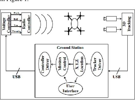
The control environment used here consists of a commercial MAV observed by a 3D tracking sensor, whose information is transmitted via a serial link to a soft real-time application running on a ground-station. The application performs target recognition in the 2D view of the scene using machine vision algorithms, and retrieves vertical, horizontal, the depth co-ordinates for the identified target. This data is fed to mission-management and control algorithms, and calculated pitch, roll, yaw and throttle commands are directly inserted as raw voltages into the four-channel joystick interface of the MAV’s standard manual control unit, via a serially connected Digital-to-Analogue Convertor. This architecture is summarized in Figure 1.

Figure 1: Control Environment Architecture

relying on the human operator to perform visual lati-tude, longitude and altitude position control: the tracking and control application therefore assumes the role of this operator.

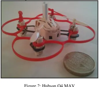
Figure 2: Hubsan Q4 MAV

The control application performs target discrimina-tion by a two-stage process. The image is pixel-wise filtered for relative content of primary red, and com-pared to a threshold to render a black/white image containing all red-hued objects in the scene. In the second stage, machine-vision algorithms are applied to identify all individual continuous objects, allowing the largest in the scene to be selected as the target. Figure 3 illustrates the output of this process in the application’s user interface, with the selected target having been highlighted and smaller candidate ob-jects rejected.

Figure 3: User Interface Target Display

A Microsoft Kinect 1.0 is used to provide basic 2D scene imagery and depth perception by painting of the scene with infra-red-illuminated tags for viewing via IR-filtered stereo vision [1]. In order to provide a discernable target for both the image recognition and

depth perception sensor functions, a square target marker is mounted above the centre of gravity of the airframe. Data is fed to the ground-station via a Uni-versal Serial Bus (USB) connection. The marker is colored primary red in order to allow clear discrimi-nation of the target in the scene image with simple image recognition algorithms, and sized 5cm square in order to allow the Kinect’s relatively granular depth perception functionality to operate. All control functions such as image recognition, depth extraction, control loop closure, wireless interface communica-tions, and user interface are implemented as a single coded in the C# language [10] and application run-ning on Windows 7. The user interface allows con-figuration of basic flight parameters such as desired altitude and flight time, provides feedback of the sce-ne image (shown in Figure 3) in full-spectrum, red-filtered, and depth coloration, and displays traces of position and velocity in each dimension (shown in Figure 4).

Figure 4: User Interface Vertical Trace

Verifica-tion is therefore required, which is performed by stat-ic calibration of the tracker equipment using place-ment of the target marker in measured 3D positions across its viewing range. Using this approach, the system was shown to maintain a resolution of 5mm across the operational range.

Thus, by the use of commonly available consumer and development hardware and freely available open-source software, the complete control environment is implemented at a cost below £100. The equipment comes with functional compromises: the soft real-time behaviour demanded by the use of C# on the Windows platform, 5cm target size demanded by the first-generation Kinect tracker, and primary red target color used to simplify target discrimination with the simple machine-vision algorithms used. More signifi-cant are performance restrictions: computational load and un-optimized software restrict the equipment to a 0.1 second iteration period and 0.3 second data laten-cy. These issues are representative of future distribut-ed ground-basdistribut-ed MAV control issues, and provide a useful platform for their investigation. Nonetheless, refinement of the system to reduce many of these issues is in progress.

3.Development Process

Initial flights of the MAV in the development envi-ronment confirmed that, even in the controlled condi-tions of an MAV in a laboratory, unpredictable fac-tors still render systematic controller development using an actual airframe impractical. Most significant of these are ground-effect (the increased lift and de-creased induced drag when close to a surface) and unpredictable battery performance during discharge [15]. Thus the development cycle familiar to devel-opers of large-scale aircraft was adopted, namely construction of a dynamic model in a simulated envi-ronment, based on empirical airframe data (analogous to wind-tunnel derived data for large aircraft). This model was then verified against flight-test data using open-loop controller settings and used for develop-ment of a closed-loop algorithm. This process in-cludes the use of the Mathworks Simulink tool [16], the de-facto standard for system modelling and con-troller development in the aerospace industry. Once a candidate closed-loop algorithm was constructed, it was then re-implemented and verified in the flight-test environment.

3.1.Dynamic Model

The model is constructed at an intermediate level of abstraction, using a combination of pure physical theory and abstractions of empirical data. The entire modelled system may be considered in three parts: the position and velocity of the airframe (described in Section 3.2) under the action of the motorized rotors (described in Section 3.3), which are in turn modulat-ed by the controller (describmodulat-ed in Section 3.6).

3.2.Airframe Dynamics

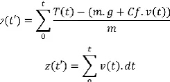
The airframe position model implements simple dis-crete mechanics of the form:

where altitude z and vertical velocity v at time t are functions of rotor thrust T, airframe mass m, ac-celeration due to gravity g, and coefficient of friction Cf.

Thus the model implementation calculates a down-ward force due to the weight of the MAV, which sub-tracts from the upward force due to the thrust of the motor/rotor propulsion subsystem. The resulting net force is divided by the airframe mass to yield an up-ward acceleration. Acceleration is integrated to yield an upward velocity and again to yield position (i.e. altitude). The intermediate velocity is also used to feedback a proportional frictional force to the net-thrust calculation. This proportional term abstracts the true squared relationship due to drag [14] in order to simplify the modelling process, but is sufficient for the relatively low speeds achieved. A simplification of the model when coded in Simulink is shown in Figure 5.

Figure 5: Airframe Dynamic Model

yields a throttle demand to the propulsion sub-system, described in Section 3.3.

3.3.Propulsion dynamics

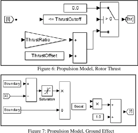
The model for the thrust generated by the MAV’s motor/rotor consists of two elements: a calculation of basic force generated by the motors and rotors for a given throttle setting, which is scaled by a multiply-ing factor due to the ground-effect at a given altitude. Both the throttle/thrust and altitude/ ground-effect relationships are modelled as simple linearized ap-proximations of empirical data (discussed fully in Section 3.4). In the case of the ground-effect calcula-tion, the effect is modelled as proportionally decreas-ing towards a threshold altitude, at which the effect is assumed to cease. One element of the propulsion sub-system that is not modelled in detail is the effect of battery discharge with use, leading to loss of thrust for a given throttle setting. The throttle/thrust and altitude/ ground-effect elements of the model, coded in Simulink, are shown in Figure 6 and Figure 7 re-spectively.

Figure 6: Propulsion Model, Rotor Thrust

Figure 7: Propulsion Model, Ground Effect

For both the airframe and propulsion models, all pa-rameters describing a particular MAV are encapsulat-ed in a separate initialization file, allowing the model to be rapidly reconfigured for other airframes. For the altitude control investigation at the level of abstrac-tion chosen, the only parameters needed are the air-frame’s mass, the altitude of the ground-effect boundary (at which the ground-effect ceases), the ground-effect thrust multiplier (defining the increase in thrust at zero altitude due to ground-effect), and a

ratio/offset describing the thrust generated for a given throttle setting. For any given airframe control unit, the throttle will be an arbitrary interface depending on the nature of the controller: in the case of the Hub-san Q4 demonstration, the throttle input is a continu-ous voltage in the range 0-3.3V. The final parameter is the frictional coefficient (defining a proportional frictional force for a given velocity).

3.4.Model Parameterization

As discussed in Section 3.1, the model is derived by a combination of theory and empirical data, and both of these require appropriate parameterization for a given test article. In the simplest case, the essential parame-ter of the MAV’s mass (including its attached track-ing target) is measured directly ustrack-ing a jeweller’s balance with 0.1g resolution.

Other essential parameters are measured using a simple system identification rig in which the MAV is mounted via an overhead rod, transmitting the net vertical force into the same jeweller’s balance, shown in Figure

8

Figure 8: System Identification Test Rig

This rig gives sufficient accuracy and resolution for the forces being considered. One notable feature of the rig is the vertical arm and slender suspending rod within an unobstructed airspace above and below the airframe, in order to minimize interference effects due to turbulence. This configuration was adopted after early experiments with underside-supported apparatus suggested that surface interactions were causing significant measurement errors.

charged), generated using the rig, are plotted in Fig-ure 9.

Figure 9: Throttle/Thrust Characteristic

The most significant features of this data are the clear linear relationship between throttle and thrust throughout the usual operating range for MAV flight, and the relatively low change of thrust across the major period of battery discharge. Thus, the throt-tle/thrust relationship could be modelled by a simple ratio/offset formula and a single representative char-acteristic selected for all battery discharge levels.

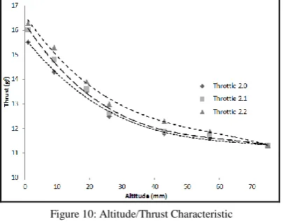
A similar technique was applied to characteriza-tion of the ground-effect relacharacteriza-tionship: thrust was measured for a range of throttle settings at different static altitudes above the take-off surface. For exam-ple, the relationships for three throttle settings (at 100% battery capacity) within the operating range are plotted in Figure 10.

Figure 10: Altitude/Thrust Characteristic

As discussed in Section 3.3, this data suggested that an approximation of a linear roll-off of ground-effect from approximately 30% at ground-level towards 0% at the ground-effect boundary was adequate. For the Q4 test airframe, this cutoff boundary was found to be at approximately 5cm. Static mounting of the MAV on the system identification rig precluded di-rect measurement of the velocity drag coefficient, and

this figure had to be derived indirectly from launch trajectory data during the model verification process (described in Section 3.5). The inexact nature of this measurement is reflected in the fact that the drag force is approximated to a proportional term, as dis-cussed in Section 3.2.

3.5.Model Verification

Having constructed and parameterized an initial dy-namic model, flight-testing with static throttle set-tings was performed to verify the model’s accuracy and infer the remaining (velocity-related) frictional coefficient. A comparison of model and fight-test derived data for time/altitude is shown in Figure 11.

Figure 11: Model/Flight-Test Trajectory

The trajectory used for this verification exercise demonstrates a useful by-product of ground-effect for this exercise. A throttle setting could be selected (through theory and experiment) to result in a net upward acceleration within the ground-effect region, but downward beyond it. Thus a single throttle set-ting results in the airframe being launched, before describing a parabolic trajectory back to near ground level. Curiously, at this point the airframe rebounds before reaching the take-off surface, due to the in-crease in rotor thrust (proportional to the airframe’s penetration into the ground-effect region) being suffi-cient to overcome the airframe’s downward motion and then reverse its direction. This effect was demon-strated in both simulated and flight-test environments.

describing the ground-effect boundary and frictional coefficient.

3.6.Controller Development

Having constructed a verified dynamic model, devel-opment of a control loop could proceed in this con-trolled and consistent simulated environment. A min-imal control law was implemented to control the MAV to a stable selected altitude. The loop computes a desired velocity proportional to positional error, feeding into a Proportional/Integral (PI) controller, yielding a desired throttle setting. The control law, coded in Simulink within the simulated environment, is shown in Figure 12.

Figure 12: Control Law in Simulation Environment

Thus the first application of the dynamic model was discovery of the proportional and integral gains for the controller. In classic control theory, the integral term may be considered as cancelling out any steady-state error: in the context of this algorithm, this corre-sponds to the constant demand required to neutralize the weight of the airframe, allowing its vertical movement to be controlled by proportional-term off-sets from this datum value. As this offset “error” may be reliably predicted, the integrator may be initialized to the airframe weight (i.e. product of its mass and g) without the need for the integrator to be dynamically initialized, giving improved performance immediate-ly after startup.

However, in common with many practical control systems, a major element of the controller develop-ment is accommodation of the sample-and-hold effect of a discretely sampled system, and latency within the sensing and actuation devices of the platform. As discussed in Section 2, for this example the practical limitations of the control equipment implied an itera-tion period of 0.1 seconds and sensor latency of 0.3 seconds. Thus an essential requirement for the simu-lated controller environment was correct modelling of these effects in order to allow them to be overcome.

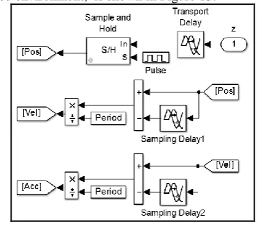
This element of the controller, modelled in the simu-lated environment, is shown in Figure 13.

Figure 13: Simulated Controller Interface

Due to the issues of discretization and latency, intro-duction of predictive models for estimating actual position and velocity from the delayed data were es-sential for loop closure. For the initial control law described here, simple linear extrapolation of position and velocity based on observed velocity and accelera-tion respectively was sufficient.

As expected, the properties of the ground-effect region rendered the assumptions implicit in the gains of the basic PI control law ineffective, and this pre-sents a rich subject of future study. In order to pro-ceed with practical flight-testing a simple timed open-loop throttle setting was introduced to manage take-off, projecting the airframe rapidly out of the ground-effect region before engaging the closed-loop PI law.

3.7.Controller Implementation

Provision of flight-test infrastructure for the system identification, modelling and verification phases had driven the development of necessary airframe track-ing, control, and instrumentation functions needed to support full control loop closure, making this step relatively trivial.

Figure 12 is implemented by the pseudo-code section shown in Figure 14.

Figure 14: Control Law Implementation

3.8.Controller Verification

Having implemented the theoretical control law, veri-fication could be performed by comparison of auto-matically generated spreadsheet data from each tool. Altitude data for a climb to a desired altitude of 0.4 metres for both simulated and actual flight-test launches are shown in Figure 15.

Figure 15: Comparison of Altitude Profiles

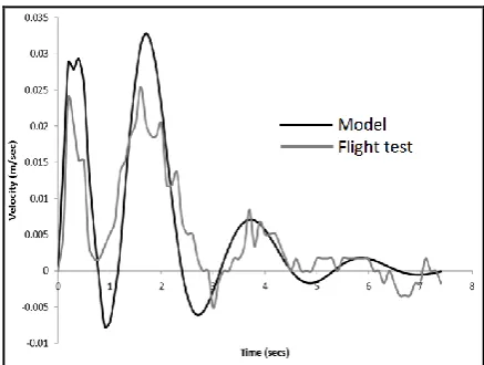
The data shows an initial rapid acceleration of the airframe due to ground-effect, followed by a loss of momentum before the PI controller engages to con-trol to the desired altitude. Comparative plots of ver-tical velocity (i.e. first derivative of altitude) for the same flight are shown in Figure 16.

Figure 16: Comparison of Vertical Velocity Profiles

This figure emphasizes the more unsteady trajectory of the flight-test example due to variations in thrust, turbulence in the airspace, and resolution limitations in the visual tracking equipment.

3.9.Analysis of Results

Once refined in simulation, final flight-testing of both the open and closed loop controller algorithms show close correlation between simulated and flight-test trajectories, confirming the adequacy of the model and validity of the development process.

The basic PI control loop implemented here was a deliberately minimal solution for achieving stable altitude, in order to reveal the practical considerations necessary for remote ground-based control. These results clearly demonstrate the two most significant considerations: loop sensor/actuator latency and throttle/thrust non-linearity due to ground-effect. The linear predictive filter introduced to counter sensor latency is adequate for the small accelerations com-manded by the current PI loop, but is unlikely to be sufficient for more rapid maneuvers. Similarly, en-hancements to the control loop itself are required to manage controlled flight within the ground-effect region.

static measurement of thrust at each altitude may overlook dynamic effects, and comparison with data derived from flight-test launches should be investi-gated.

The results illustrate the very sensitive nature of controlling altitude in thrust-supported vehicles such as quadcopters. The majority of the propulsive thrust is expended in countering the airframe’s weight and altitude is dominated by the second integral of a val-ue that is itself the difference of two large numbers. For example, commanding a violent vertical accelera-tion requires a throttle increase of only approximately 5% above the nominal value required for static hover-ing flight.

Despite the varying initial conditions due to the launch process, the simple closed control loop im-plemented proved to be sufficiently robust to ac-commodate battery discharge once outside the ground-effect region.

This investigation focuses on control of only one DoF in isolation, and it is important to acknowledge the challenges of expanding its scope to include other DoFs [8]. For example, the linear predictive model used here is insufficient for handling simultaneous lateral control, as the loss of vertical thrust due to pitch and roll maneuvers is not considered. For more rapid maneuvering, more advanced issues such as gyroscopic coupling between DoFs should also be considered.

4.Conclusions & Future Work

Automatic ground-based visual control of a very low weight (15g) MAV has been demonstrated for a con-trol iteration period of 0.1 seconds, a sensor/actuator latency of 0.3 seconds, and ground-effect induced throttle/thrust non-linearity at altitudes below 50mm. A model-based approach was shown to be essential in order to overcome these dominant issues: latency compensation using appropriate real-time predictive modelling being essential to achieve closed-loop con-trol, and understanding of ground-effect being essen-tial for achieving of stable launch.

In spite of its vastly greater simplicity compared to that for large airframes, it has been shown that even MAV flight testing is too unpredictable for effi-cient system development, and construction of ade-quate dynamic modelling is needed, in this case using a combination of fundamental physics and empirical system identification. There is no substitute for a

model-verify-develop-deploy cycle, and resources invested in model development are richly rewarded.

As stated at the outset, the investigation described here represents the first phase of a larger roadmap, and much continuation work is either envisaged or already in progress, focusing on improvements to the MAV dynamic model and its corresponding ground-based controller. Dynamic model improvements are envisaged in modelling of ground-effect, dynamic drag, and the effects of battery discharge: all of which are enabled by the stable launch capability and sys-tem identification rig described here. These model improvements shall in turn enable development of more resilient control algorithms, combining other DoFs, and employing more detailed models [1][3] and system identification methods [21]. The tools developed for this investigation are intended from the outset to be retargeted to other airframes, and control of other quadcopters [9] is planned.

References

[1]Alkowatly M.T., Becerra V.M., Holderbaum W. (2014) "Body-centric Modelling, Identification, and Accelera-tion Tracking Control of a Quadrotor UAV" Interna-tional Journal of Modelling, Identification and Control, Volume 21, Issue 1, pp 29-41

[2]Baek J-Y, Park S-H, Cho B-S, Lee M-C (2015) "Position Tracking System using Single RGB-D Camera for Evaluation of Multi-Rotor UAV Control and Self-Localization" IEEE International Conference on Ad-vanced Intelligent Mechatronics, pp 1283-1288 [3]Bellocchio E, Ciarfuglia T.A., Crocetti F, Ficola A, Valigi

P (2016) "Modelling and simulation of a quadrotor in V-tail configuration" International Journal of Modelling, Identification and Control, Volume 26, Issue 2, pp 158-170

[4]Bošnak M, Matko D,Blažič S (2012) "Quadrocopter Hov-ering Using Position-estimation Information from Iner-tial Sensors and a High-delay Video System" Journal of Intelligent & Robotic Systems, Volume 67, Issue 1, pp 43-60

[5]Bristeau PJ, Callou F, Vissiere D, Petit N (2011) “The navigation and control technology inside the ar. drone micro uav” 18th IFAC world congress, pp 1477-1484 [6]Clark R, Punzo G, Dobie G, Summan R, MacLeod CN, Pierce G, Macdonald M (2014) "Autonomous swarm testbed with multiple quadcopters" , 1st World Con-gress on Unmanned Systems Enginenering

[7]Cypress Semiconductor (2012) "PSoC5: CY8C55 Family Datasheet" Cypress Semiconductor Corporation, San Jose, CA, USA

[8]Das A, Subbarao K, Lewis F (2008) "Dynamic inversion with zero-dynamics stabilisation for quadrotor control" IET Control Theory & Applications, Volume 3 Issue 3, pp 303-314

Nano-Quadrotor” IROS2014 Aerial Open Source Robotics Workshop

[10] Hejlsberg A, Wiltamuth S, Golde P (2003) "C# Lan-guage Specification" Addison-Wesley Longman, Bos-ton, MA, USA

[11] Huang AS, Bachrach A, Henry P, Krainin M, Maturana D, Fox D, Roy N (2011) "Visual Odometry and Map-ping for Autonomous Flight Using an RGB-D Camera" International Symposium on Robotics Research [12] Kim K, Kim W, Choi D, Myung H (2015) "Calibration

of the drift error in GPS using optical flow and fixed reference station" 15th International Conference on Control, Automation and Systems, pp 1370 - 1373 [13] Kushleyev A, Mellinger D, Powers C, Kumar V (2013)

"Towards a swarm of agile micro quadrotors" Autono-mous Robots, November 2013, Volume 35, Issue 4, pp 287-300

[14] Leishman R, Macdonald J, Beard R, McLain T (2014) "Quadrotors and Accelerometers: State Estimation with an Improved Dynamic Model" IEEE Control Systems, Volume 34, Issue 1, pp 28-41

[15] Linden D, Reddy TB (2002) "Handbook of batteries" McGraw-Hill, New York, USA

[16] Mathworks (2015) “Simulink User's Guide” Mathworks Inc., MA, USA

[17] Mathworks (2015) “Simulink Coder User's Guide” Mathworks Inc. , MA, USA

[18] Mustapa Z, Saat S, Husin S, Abas N (2014) “Altitude controller design for multi-copter UAV” International Conference on Computer, Communications, and Con-trol Technology, pp 382-387

[19] Naidoo Y, Stopforth R, Bright G (2011) "Quad-rotor unmanned aerial vehicle helicopter modelling & con-trol" International Journal of Advanced Robotic Sys-tems, Volume 8, Issue 4

[20] Tanenhaus M, Carhoun D, Geis T, Wan E (2012) "Min-iature IMU/INS with optimally fused low drift MEMS gyro and accelerometers for applications in GPS-denied environments" Position Location and Navigation Sym-posium (PLANS), 2012 IEEE/ION