Mixing tone mapping operators on the GPU by differential zone mapping based on psychophysical experiments

Mixing Tone Mapping Operators on the GPU

by Di↵erential Zone Mapping Based on

Psychophysical Experiments

Francesco Banterle

, Alessandro Artusi

, Elena Sikudova

,

Patrick Ledda

, Thomas Bashford-Rogers

, Alan Chalmers

,

and Marina Bloj

1

ISTI-CNR, Italy

2

Universitat de Girona, Spain

3

Comenius University, Bratislava, Slovakia

4

MPC Ltd, UK

5

University of Warwick, UK

6

University of Bradford, UK

October 19, 2016

Abstract

In this paper, we present a new technique for displaying High Dy-namic Range (HDR) images on Low DyDy-namic Range (LDR) displays in an efficient way on the GPU. The described process has three stages. First, the input image is segmented into luminance zones. Second, the tone mapping operator (TMO) that performs better in each zone is automatically selected. Finally, the resulting tone mapping (TM) out-puts for each zone are merged, generating the final LDR output image. To establish the TMO that performs better in each luminance zone we conducted a preliminary psychophysical experiment using a set of HDR images and six di↵erent TMOs. We validated our composite technique on several (new) HDR images and conducted a further psy-chophysical experiment, using an HDR display as the reference, that establishes the advantages of our hybrid three-stage approach over a traditional individual TMO. Finally, we present a GPU version, which

is perceptually equal to the standard version but with much improved computational performance.

Kewyowrds: High Dynamic Range Imaging, Tone Mapping Op-erators, Real-Time Tone Mapping, and GPU Programming.

1

Introduction

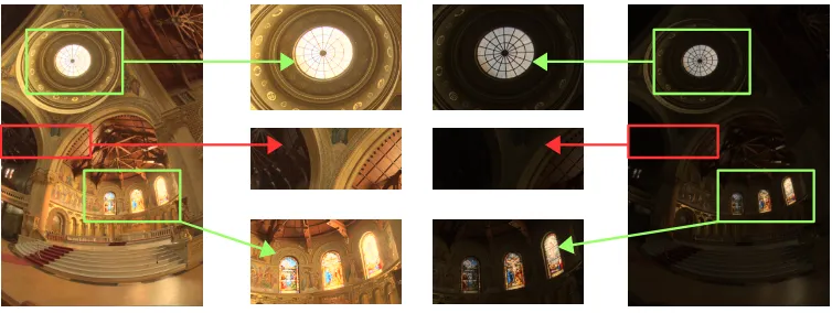
The growth of the HDR imaging has led to the development of a variety of TMOs that attempt to simulate di↵erent aspects of the Human Visual System (HVS). The intent is to solve issues, such as preserving local contrast, avoid-ing halo artifacts, simulatavoid-ing visual adaptation, enhancement and expansion of the original dynamic range, contrast reduction, image detail preservation, etc. Figure 1 shows how two TMOs attempt to reproduce two di↵erent as-pects such as the contrast and the detail: the left side of Figure 1 shows how the detail is well reproduced in the windows, but the contrast is not preserved. The right side of Figure 1 shows how the contrast is preserved in the bright (see the green squares) and dark areas (see the red squares) but the details are not well reproduced (see the windows).

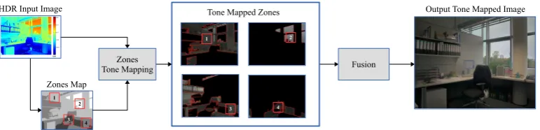
At the time of writing, two main problems remain unsolved. First, choos-ing the proper TMO for a specific application can be difficult. Second, a comprehensive TMO that takes into account all aspects specified above has not yet been developed. Motivated by these two open issues, we present a new technique for retargeting HDR images into LDR display that takes into account the benefits of di↵erent existing TMOs and combines them, result-ing in a more perceptually accurate image compared to the images obtained by existing TMOs. Figure 2 depicts our framework. We decomposed, based on the luminance characteristics, the input HDR image into zones and ana-lyzed the benefits of six di↵erent TMOs for each luminance zone. The TMOs that perform better in each luminance zone were selected. This step, based on human observations, and on the specific application where the TMOs are required to be applied, is able to choose the most appropriate TMO for the specific luminance zone. Finally, the results of the selected TMOs are combined to reproduce the final output LDR image. We demonstrate the re-sults of our hybrid approach on several HDR images. Using an HDR display, showing the original HDR image as reference, we conducted a psychophysical experiment that clearly shows the advantages of our hybrid approach over using a traditional single TMO.

This paper extends the previous work by Banterle et al. [12], with the following:

combin-ing strategy proposed by Yeganeh and Wang [48]; see Section 5 and additional material1_.

2. An approximated GPU-friendly version of the whole algorithm that enables a speed-up of 100 times on average; see Section 6.

3. An evaluation of the GPU-friendly version; in order to estimate if the proposed approximations produce or not an identical result compared to the original algorithm; see Section 6.4 and additional material2_.

4. A GPU-friendly approximation of the local Photographic Tone Map-ping Operator that works in real-time with HD, 4K, and 8K content; see Section 6.2.

The rest of the paper is organized as follows: Section 2 describes related work. Section 3 presents our technique. Section 4 presents the pshychophys-ical validation of our method, and Section 5 presents comparisons against the state-of-the-art. Section 6 shows how to approximate the algorithm for graphics hardware and evaluates its performance and quality. Finally, Sec-tion 7 concludes and presents future work.

2

Related Work

The concept of tone mapping in computer graphics was introduced by Tum-blin and Rushmeier [43], who proposed a tone reproduction operator that preserves the apparent brightness of scene features. Subsequently, many TMOs have been proposed. It is not the purpose of this paper to give a complete overview on HDR imaging and TM techniques. For a full overview see [37, 11, 9, 10]. In this section, we will review only the approaches that are related to our work.

TMOs, that make use of segmentation to identify regions in the input image with common properties, are not new in the field of computer graphics. For example, the histogram adjustment proposed by Ward et al. [46], was one of the first operators presented that belongs to this group of algorithms. This operator divides an image into bins and equalizes its histogram. However, it does not make use of the spatial information in the segmented areas for further compression of the dynamic range.

1_{http://www.banterle.com/work/papers/ic_hybrid_tmo/additional_our_vs_}

attm.pdf

2_{http://www.banterle.com/work/papers/ic_hybrid_tmo/additional_cpu_vs_}

Figure 1: Example of two TMOs that take into account two di↵erent aspects. On the left side, the contrast in the bright (green squares) and dark areas (red square) is preserved but the detail in the windows is not well reproduced. On the right side, the detail in the windows is well reproduced (i.e., the global contrast is well reproduced), but the detail in the dark areas are not preserved. The original image is copyright of Paul Debevec.

Yee and Pattanaik [47] presented a model that makes use of the spa-tial information. The HDR image is segmented into bins in the logarithmic space, pixels are labeled into groups, and the local adaptation luminance is calculated for each group. Finally, the local adaptation luminance is used to compress the dynamic range of the input image.

Krawczyk et al. [29] proposed a perceptual approach that leverages the an-choring lightness perception theory [25]. Their operator segments the image in frameworks, using a k-means approach, and calculates for each framework a weight map. After this step, for each framework the anchoring is calcu-lated, and the frameworks are merged together using the weight maps. We have used a faster and simpler segmentation approach and a simple binary map in the fusion step. It is true that our segmentation approach may gen-erate superficial boundaries between segments but this problem is addressed by the use of our blending technique.

A user centered approach was investigated by Lischinski et al. [33]. In their method a soft segmentation is generated using rough brushes created by the user. Each brush determines the exposure that the user chose for the specific area. Then, the di↵erent exposures areas are merged to create the output image. The authors also proposed an automated initialization version of their approach, but user intervention is not completely eliminated due the interactive nature of their approach.

ex-Zones Tone Mapping

1 4 2

Fusion HDR Input Image

Zones Map

Tone Mapped Zones Output Tone Mapped Image

3

2 1

4 3

Figure 2: Schematic description of our framework. First, the HDR input image is segmented into luminance zones and a zone map is created. Sec-ond, the optimal TMO for each zone is applied on the whole input image generating di↵erent output images; i.e., one for each zone. Finally, the tone mapped images are merged and the final output is generated. For visual-ization purposes, we only show the specific zone tone mapped in the Tone Mapped Zones. The original image is copyright of Ahmet O˘guz Aky¨uz.

posures without the generation of an HDR image. This method, for each exposure, generates a weight map of pixel well-exposed, which can be seen as a soft segmentation. Exposures are merged using these weight maps and Laplacian pyramids blending is adopted for avoiding seams. In our case, the weight map is a simple binary map and can be easily generated and further acceleration of our approach is straightforward (see Section 3.3).

Cadik [16] presented a perceptual motivated approach that is based on combination of arbitrary global and local tone mapping operators. This tech-nique must carefully select the local and global TMOs in order to reproduce high quality output images and this selection is not based on human obser-vation.

Artusi et al. [7, 4] introduced the concept ofselective tonemapper that is based on some drawbacks of visual attention approaches [6]. In this model, the local luminance adaptation is computed only in high frequency regions. The resulting luminance image is afterwards compressed for a LDR display by using a global tone mapping curve. This avoids the typical drawbacks of a merging step (i.e., seams) when tone mapping an HDR image with two di↵erent TMOs (local and global), and greatly reducing computations.

and Wang also proposed to blend di↵erent TMOs based on the index using Laplacian pyramids, in a very similar fashion to Banterle et al.’s work [12]. The blending is driven by quality index values of tone mapped images; these are computed per pixel for each TMO.

Recently, Boitard et al. [15] presented a video tone mapping operator that preserves the temporal brightness coherency locally. First, the operator segments each frame of a video into zones using the frame log-luminance histogram with constant boundaries. Second, a key value for each zone in the current frame is computed. Third, Boitard et al.’s algorithm [14] is applied for each zone, and blending is applied to avoid artifacts at zones’ boundaries. Authors showed that this method can preserve both spatial and temporal local brightness coherencies and they validated it with a subjective evaluation. Note that this method, as Krawczyk et al.’s one [29], is not spatial, and a spatial grouping is important to help experiment participants to evaluate zones without the need to take into account isolated few pixels.

In this work, we also present a novel GPU implementation of Reinhard et al.’s operator [38]. GPU acceleration of TMOs have started in the last decade proposing general frameworks [5, 4] or TMO-specific implementa-tion [27, 39, 2]. Compared to the previous work, we present a TMO-specific implementation where its strength resides in the fact that only a single GPU pass is required in order to tone map an image making the algorithm mem-oryless. This is thanks to the use of an efficient in terms of memory and computational speed bilateral filter [13].

The solution proposed in this paper, does not need user intervention, takes into account spatial information, and it is validated via a psychophysical study where the original HDR image is shown on an HDR display.

3

Algorithm

Our Framework, as illustrated in Figure 2, can be separated in three straight-forward steps. First, we segment the input HDR image into luminance zones and a zone map is generated. Second, for each zone we choose a TMO and apply it on the whole input image generating di↵erent output images; i.e., one for each zone. Finally, we merge the resulting outputs for each zone. In the following subsections, each step is described in detail.

3.1

Zone Map Generation

magnitude value as

Z(x) =



log10L(x) , (1)

where L(x) is the luminance value of the image at pixel x, and [_·] is the rounding operator. However, the resulting Z can have very small isolated areas, even a few pixels, that are difficult to evaluate during our psychophys-ical experiments; see Section 3.2. Therefore, based on the display spatial resolution used in our experiments, we decided to merge small isolated areas that size is below 5% of the image size. From the smallest isolated area to largest one (below 5% area threshold), the merging function assigns a small isolated area to its spatially closest neighbor area with the closest dynamic range. This process stops when there are no more small isolated areas in Z; see Figure 3 (b). Connected components algorithm [26] is employed to determine isolated small areas and neighbor queries.

Note that more sophisticated approaches can be employed. For example, we tested SuperPixels [1]; see Figure 3 (c). The e↵ort to use a more so-phisticated approach when generating Z may produce better quality zones. However, in our experiments, we found out that extra computational e↵orts are not going to impact on the large areas but only at the boundaries of the zones; see Figure 3 (b) and (c).

(a) (b) (c)

Figure 3: A zone map output from an HDR image: (a) a zone map with noisy areas as result of our thresholding approach; (b) the zone map in (a) after merging and removing small isolated regions; (c) a zone map generated using SuperPixels [1]. The original image is copyright of Ahmet O˘guz Aky¨uz.

3.2

Tone Mapper Selection

Our main goal is to show that is possible to select, based on human obser-vations, a number of existing TMOs and use a combination of their results to reproduce an output image that takes into account all the advantageous aspects of single TMOs. In order to identify which TMO performs better in a specific luminance zone, we conducted a series of psychophysical experiments. To prove the concept above and be able to generalize its validity, we chose a subset of TMOs from literature. These TMOs were selected based on the previous work by Ledda et al. [32]. Therefore, in our work we investigated the following six TMOs: the algorithm proposed by Tumblin et al. [42]; the histogram model presented by Ward et al. [46]; the time-dependent visual adaptation model [35]; the photographic model (local operator) [38]; the bi-lateral filtering in the context of TM [22]; and finally, the model presented by Drago et al. [21]. The TMOs are implemented as provided in [37], using the default parameters for each operator. In the case of the operator pre-sented by Pattanaik et al. [35], which takes into account the time dependency adaptation of the HVS, we used only the final frame of the adaptation pro-cess. We have chosen these operators based on their quality performances, usability, and popularity. We also limited the number of TMOs tested based on the fact that the purpose of this paper is to prove the concept and not to have a complete comparison of the qualities of the all existing TMOs in the computer graphics community. The iCAM method [24] was originally included but some of the generated images had a violet tinge that did not entirely disappear even adopting the solution suggested by the authors [23]. Note that using a single TMO and varying its parameter values for each zone is not a suitable approach. The parameters are difficult to manually choose. In fact, this process can be very time consuming, because TMOs can have more than 3-4 parameters making the space exploration a tedious task for a user. On the other hand, an optimization process can be employed to find TMO parameters, but it can be computationally expensive. For example, generating the tone mapped images for all zones in Figure 4 requires 254 seconds using TMQI [48] as function goal of the optimization process and Drago et al. operator as TMO. Moreover, an optimization process can fail to determine parameters that are suitable for merging di↵erent zones into a single picture; see Figure 4. In fact, it can get stuck in local minima.

3.2.1 Set-up

Zone -1 Zone 0 Zone 1 Zone 2 Zone 3

O

pt

im

iz

ed

T

M

I

m

ag

e

Z

on

e

M

as

k

Optimization Merge

Figure 4: An example of an optimization process (using TMQI as maxi-mization goal) to determine for each zone the parameters of a Drago et al. operators. In the green box, the tone mapped images (bottom) for each cor-responding zone (top). In the red box, the result of merging all tone mapped images using Laplacian pyramids and each zone mask as weight (top in the green box) for the corresponding tone mapped image (bottom in the green box). Note that the merging result can produce posterized areas (blue boxes). This is because a TMO may be not suitable for certain dynamic range zones, and the optimization process may struggle in finding high quality results.

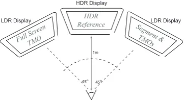
compared psychophysically. We performed this test using a Dolby DR37-P HDR display [19] and two LDR LCD displays - which are identical to the front panel of the HDR display. All have a resolution of 1920_⇥1080 pixels. In these experiments, we used the set-up shown in Figure 6. The reference HDR image was presented on the HDR display (center). On the LDR display on the right, all of the LDR images obtained with the six TMOs together with the luminance zone map were displayed. By selecting one of the six images on this monitor, a full size version could be seen on the LDR display on the left. The specific luminance zone under examination was outlined in red on the luminance zone map and on both the HDR and full size LDR images. This outlining ensured that the observer was aware of the particular zone currently being evaluated. The participants could take as much time as they required to complete the task.

were clipped around 3000 cd/m2_{. Moreover, due to the flanking displays, a}

veiling e↵ect can appear on the reproduced images. This problem was taken into account. A pilot experiment demonstrated that making use of a proper distance between each LDR and the HDR displays (half meter) avoided this problem.

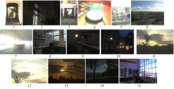
Figure 5: Images used in the psychophysical experiment. The number under the image corresponds to the numbers in the Table 3.2.1. Images 1-3 and 11-13 are copyright of Patrick Ledda. Images 4-10 and 14 are copyright of Ahmet O˘guz Aky¨uz. Image 15 is copyright of Fredo Durand.

The luminance zones available on the HDR display cover the range from 10 2_{to 3⇥10}3 _cd/m2_{. The images, used in our experiments (see Table 3.2.1),}

cover the range from 10 2 _{to 10}3 _cd/m2 _{as shown in the Table 3.2.2. The}

participants were asked to select the TMO that was considered to reproduce the results as close as possible to the HDR reference image in a specified luminance zone. A group of 24 na¨ıve participants between 20 and 60 years old with normal or corrected to normal vision took part in this experiment. The display was placed in a dark room minimizing the e↵ects of ambient light. Prior to the start of the experiment, each participant was given five minutes to adapt to the environment.

3.2.2 Data Analysis

In our task, observers were asked to indicate for a given image and zone which of the six TMOs was closer to the reference. This includes not only luminance contrast, but also fine details reproduction and color information. Since the observers did not rank all the algorithms we do not have ordinal data but rather categorical data. This allows us to use one-variable 2 _test

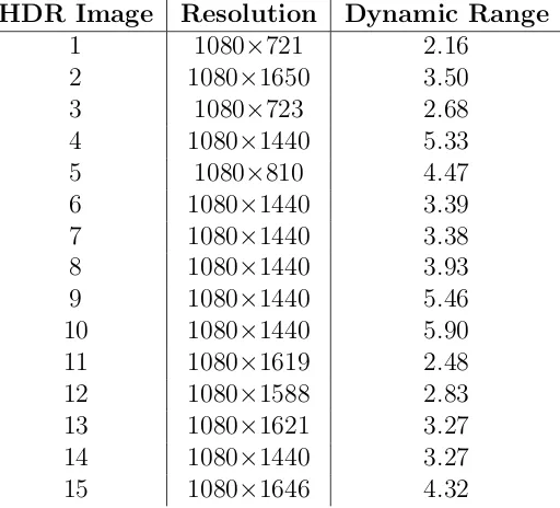
HDR Image Resolution Dynamic Range

1 1080_⇥721 2.16 2 1080⇥1650 3.50 3 1080⇥723 2.68 4 1080_⇥1440 5.33 5 1080⇥810 4.47 6 1080⇥1440 3.39 7 1080_⇥1440 3.38 8 1080⇥1440 3.93 9 1080⇥1440 5.46 10 1080_⇥1440 5.90 11 1080⇥1619 2.48 12 1080⇥1588 2.83 13 1080_⇥1621 3.27 14 1080⇥1440 3.27 15 1080⇥1646 4.32

Table 1: Images used in the psychophysical experiment for the evaluation of the TMOs in the specific luminance zone. The dynamic range is expressed as order of magnitude (logarithm base with base ten of the dynamic range).

on a row in Table 3.2.2) is significantly di↵erent from that which we would expect if participants showed no di↵erence (all scores would be 100/6 = 16.6 %).

Zone TMO 1 TMO 2 TMO 3 TMO 4 TMO 5 TMO 6 2

3 28% 22% 23% 1% 20% 6% 78.23

2 23% 15% 31% 1% 20% 10% 98.24

1 36% 6% 32% 1% 14% 11% 138.4

0 27% 6% 33% 1% 22% 11% 72.40

-1 52% 9% 20% 0% 13% 5% 74.94

-2 68% 0% 6% 0% 26% 0% 98.35

Table 2: Statistical results of the psychophysical experiment evaluating which TMO performs best in each luminance zone. The enumeration corresponds to the followings TMOs: 1 - Drago et al., 2 - Pattanaik et al., 3 - Reinhard et al., 4 - Bilateral Filtering, 5 - Ward et al., 6 - Tumblin et al. Drago et al. operator was ranked the best in the luminance zones -2, -1, 1 and 3; and Reinhard et al. operator in the luminance zones 0 and 2.

HDR

Reference Segment

& TMOs Full Scre

en

TMO

HDR Display

LDR Display LDR Display

1m

45o

45o

Figure 6: Set-up used in the psychophysical experiment evaluating which TMO performs best in each luminance zone. An HDR display is used as reference (center). The LDR display on the right is used to display the six TMOs used in the experiments and the luminance zone under examination. The LDR on the left is used to visualize full screen the TMO that the observer selected at each time in order to perform his/her evaluation.

The number in each cell indicates the percentage of times that a particular algorithm was chosen for a given image zone. The last column of the table reports the corresponding value of the test statistic 2 _{for each image zone.}

In all casesp < 0.0001 and the degree of freedomdf = 5 (num. of categories -1). In our case the number of categories is equal to the number of TMOs used in the experiment. Our results indicate that for all image zones observers chose an algorithm over others to be closer to the reference.

Reinhard et al. [38] was always well ranked.

Concerning the work of Akyuz et al. [3] we have noticed that the number of images used is 33% less than what has been used in our experiment and this may lead to di↵erent results. Also Akyuz et al. [3] is in contradiction not only with our results, but also with the results of the others such as [49], [20], [17], [31], and [30], that confirm, either partially or completely, our results.

3.3

Fusion Results

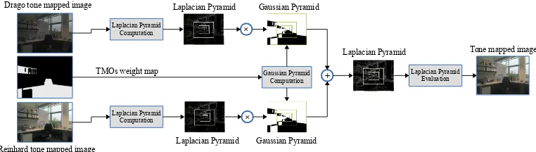
Following the results of the previous Section we concluded that the Drago et al. [21] and the Reinhard et al. [38] operators would be utilized in the fusion step. Once the TMO to be used in each zone has been selected, the di↵erent TMOs are applied to the relevant zone and the outputs are blended to create the whole image. The blending operation is necessary to eliminate discon-tinuities in the luminance, that may occur at the edges of the zones within the map. A na¨ıve blending of TMOs, is a simple multiplication of a weight map times the TMO with a consequent accumulation. This method creates artifacts such as seams and discontinuity at edges. To avoid these problems we blend the various TMOs using Laplacian blending, similar to that used in [34]. Note that the use of Laplacian blending helps masking contouring, which may appear when applying spatial blending without the need to use more sophisticated approaches for segmentation; i.e., soft segmentation [40]. This allows us to keep a straightforward approach to implement that can be implemented on the GPU; see Section 6.

Laplacian Pyramid

×

×

Gaussian Pyramid

Gaussian Pyramid Computation Laplacian Pyramid

Computation

Laplacian Pyramid Computation

Laplacian Pyramid Evaluation +

Laplacian Pyramid Gaussian Pyramid

Laplacian Pyramid Drago tone mapped image

Reinhard tone mapped image

TMOs weight map

Tone mapped image

Figure 7: Graphical representation of the fusion step of our Framework. The original image is copyright of Ahmet O˘guz Aky¨uz.

pyramid is generated. Finally, from the fusion pyramid the output image is reconstructed (Fused Result).

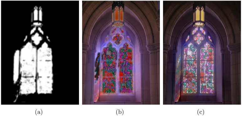
Based on the fact that the subjects’ evaluation of the TMOs in the specific luminance zone, is equivalent to give the same weight to all the pixels of the zone, we decided to use a simple Gaussian filtered binary map. We also investigated if a simple linear combination fusion scheme was able to give comparable results to the one obtained with the proposed fusion scheme. As is shown in Figure 8, several artifacts are visible in the output obtained with the simple fusion scheme (left image).

(a) (b) (c)

Figure 8: Comparison of the results obtained with two di↵erent fusion schemes: (a) the TMOs weight map; (b) a result using the simple fusion scheme; (c) a result using the proposed fusion scheme. Artifacts are visible on the image obtained with the simple fusion scheme (b). The original image is copyright of Max Lyons.

3.4

Limitations

Our method can reproduce details of di↵erent dynamic range zones with high quality. However, our proof of concept is tailored for the dynamic range available in the HDR display used in the psychophysical experiments.

HDR Image Resolution Dynamic Range

1 1016_⇥760 4.34

2 874⇥644 5.82

3 1080⇥1626 5.13 4 1080_⇥1626 4.69

5 906⇥928 4.33

6 769⇥1025 5.00 7 1080_⇥718 4.08

8 684⇥912 5.09

9 768⇥1024 3.86 10 1023_⇥767 4.53 11 768⇥512 5.40 12 1080⇥1624 4.08 13 769_⇥1025 2.45

Table 3: Images used in the psychophysical experiment for the evaluation of our TMO. The dynamic range is expressed as order of magnitude and it is covering the same dynamic range as the images used in the first experiment.

4

Results: Psychophysical Validation

In this Section we present the experimental results obtained from testing our hybrid approach.

4.1

Set-up

We tested and psychophysically validated our hybrid approach on several HDR images, using the same HDR and LDR displays as in the previous experiment. Again the HDR display was used to visualize the HDR image as the reference. We conducted a pair-wise comparison test between the two best TMOs (Drago et al. [21] and Reinhard et al.[38]) and our hybrid operator. Figure 9 shows the set-up for this experiment; the reference HDR image is displayed on the HDR display (center), and the two TMOs that are being compared are displayed on the two LDR displays. This is a similar approach to evaluating TMOs as used in [32].

HDR Reference

TM O1 TMO2

HDR Display

LDR Display LDR Display

1m

45o 45o

Figure 9: Set-up used in the validation experiment done for evaluating our hybrid TMO versus the two best TMOs of the previous psychophysical ex-periment. An HDR display is used as reference (center). Two LDR displays (right and left) are used for pairwise comparison.

Figure 10: Images used in the psychophysical experiment; the number under the image corresponds to the numbers in Table 4. Image 1 is copyright of Karol Myszkowski. Images 2 and 5 are copyright of ILM Ltd. Images 3-4 are copyright of Mark Fairchild. Image 6 and 13 are copyright of Raanan Fattal. Image 7 is copyright of Jack Tumblin. Image 8 is copyright of Francesco Banterle. Image 9 is copyright of Greg Ward. Image 10 is copyright of Max Lyons. Image 11 is copyright of Paul Debevec. Image 12 is copyright of Patrick Ledda.

experiment, are reported in Table 4 and shown in Figure 10.

4.2

Data Analysis

HDR Image First Second Third

1 HYB 26 PHO 20 DRA 17 2 DRA 37 HYB 25 PHO 1 3 HYB 38 DRA 20 PHO 5 4 PHO 30 DRA 18 HYB 15 5 HYB 30 DRA 27 PHO 5 6 HYB 26 DRA 23 PHO 14 7 HYB 34 DRA 24 PHO 5 8 DRA 35 HYB 23 PHO 5 9 HYB 30 PHO 19 DRA 14 10 HYB 38 DRA 14 PHO 11 11 DRA 34 HYB 24 PHO 5 12 HYB 31 DRA 24 PHO 8 13 HYB 30 DRA 26 PHO 7

Overall HYB 370 DRA 298 PHO 150

the di↵erence between the scores of two TMOs is considered significant if it is greater than a critical value, R [18]. In other words R represents the minimum value where the di↵erence between the scores of two TMOs is consider non-significant.

We have chosen the significance level ↵ equal to 0.05 and the critical values R is computed as:

R= 1 2Wt,↵

p

st+1

4 (2)

where Wt,↵ is the upper significance point of the Wt distribution. At a

significance level of 0.05 and for three TMOs (t = 3 the Wt,↵ is equal to

3.31; see Pearson [36], table 22). The value ofs specifies the total number of possible cases in the experiment. Table 4.1 shows the results of the second experiment.

We performed the multiple comparison range test on the results of the second experiment, for each image individually (s = num. operators) and for the combined preference over all images (s = num. operators ⇥ num. images). This test shows that overall the hybrid TMO performs significantly better than the other two TMOs used on their own. The critical valueRis 48 when evaluated over all images. Since the di↵erence in overall scores between each TMO is greater than R, the di↵erences can be considered significant.

The test results show that the hybrid operator is not significantly worse for any of the test images than the other two operators. In the cases when Reinhard et al. or Dargo et al. operators appear to have higher scores the di↵erence is less than the critical value of R, which for the case of single images is 14.

Figure 11 shows a compelling result where our method can reproduce both dark and bright regions. More results can be found in the additional material 3_.

5

Results: Comparisons against the

Adap-tive TMQI Tone Mapping

In this Section, we compared our hybrid approach against theadaptive TMQI tone mapping (ATTM) [48] (Section IV.B). This is a strategy for blending di↵erent TMOs based on their TMQI quality index using Laplacian pyramids in similar fashion to Banterle et al.’s work [12].

3_{http://www.banterle.com/work/papers/ic_hybrid_tmo/img_htmo_val_second_}

(a) (b) (c) (d)

Figure 11: A compelling example showing the efficacy of our approach: (a) Drago et al.’s method, (b) our method, (c) Reinhard et al.’s operator, and (d) the blending mask used by our method (white for Drago et al.’s method, and black for Reinhard et al.’s method).The original image is copyright of Max Lyons.

The main goal of this comparison is to determineif the strategy to select a particular TMO for each region is e↵ective as the one using the TMQI. We want to stress out that we are not interested in having the best parameters of a particular TMO but only how the blending is carried out.

In order to understand if our method has similar blending performance, we implemented ATTM using only two TMOs, Drago et al. [21] and Reinhard et al. [38], which are the same used by our approach. Furthermore we used standard parameters of TMOs in our experiments for both our method and ATTM. This was done again to reduce complexity and focusing on our goal.

(a) (b) (c) (d)

In our experiment, we tone mapped 28 HDR images Figure 10 and Fig-ure 5 using our method and ATTM. We compared each image against the original HDR image using the dynamic range independent quality assessment metric (DRIQAM) [8]. This metric is capable of operating on an image pair where both images have arbitrary dynamic ranges which makes it suitable to compare HDR images and their tone mapped counterparts [8]. The result of the metric are three maps, determining if there is an amplification, loss or reversal of the contrast in the testing image compared to the reference image. Figure 13 summarizes all results for the dataset and three maps (Please see additional material for full results). For each results (amplification, loss, and reversal), Figure 13 provides the percentage of pixels which may be de-tected by the human visual system with probability higher than 95%(P(X > 0.95)) (Please see Table.1 in the additional material4_{). From Figure 13, we}

can notice that both the tested methods, our method and ATTM, have sim-ilar performances on average with very small di↵erences.

6

Algorithm on the GPU

This section presents the GPU implementation of our method. Typically, GPU implementations have a trade-o↵ between quality and efficiency; i.e., speed and memory management. This is also valid in our case. In particular, we need to re-design the zone map and the local tone mapping operator implementations. In the next subsections, we describe the implementation details of these two steps.

6.1

Approximated Zones Map

To improve efficiency in the zone map calculations, in terms of speed, we have substituted the merging and removal of the small areas with a preprocessing filtering step. The idea underlying this design choice is based on the fact that to be merged areas are characterized by having small di↵erence in luminance values. Therefore, to merge these areas, we can smooth these di↵erences while keeping their original structure; i.e., edges. To achieve this, we can

4_{http://www.banterle.com/work/papers/ic_hybrid_tmo/additional_our_vs_}

1 5 10 15 20 25 28

Images

0 0.01 0.02 0.03 0.04 0.05 0.06

Percentage of detected pixels (%)

ATTM OUR

(a) Amplification

1 5 10 15 20 25 28

Images

0 0.1 0.2 0.3 0.4 0.5 0.6 0.7

Percentage of detected pixels (%)

ATTM OUR

(b) Loss

1 5 10 15 20 25 28

Images 0

0.005 0.01 0.015 0.02 0.025 0.03 0.035 0.04

Percentage of detected pixels (%)

ATTM OUR

(c) Reversal

apply the bilateral filter [41] for a few iterations. This filter is defined as

B(I,x, s, r) = P

y2⌦(x)I(y)Gr(kI(y) I(x)k, r)Gs(ky xk, s)

N(I,x) (3)

N(I,x) = X

y2⌦(x)

Gr(kI(y) I(x)k, r)Gs(ky xk, s), (4)

whereB is a bilateral filter,I is the input image,⌦(x) is the set of pixelsyin a window centered atx, andGrandGs are therange attenuation andspatial

attenuation functions, respectively. These are typically Gaussian functions with standard deviations r and s, respectively. Given this definition, we

iteratively apply Equation 4 in the log₁₀ domain (i.e., the same domain of segmentation). We set the filtering parameters as:

1. s = 1; we want to propagate the filtering gradually over iterations as

in a dilate/erode approach. This means a 5⇥5 wide filter.

2. r = 0.5; we want to flatten values in order to belong to a dynamic

range zone.

3. iterations =p0.05⇥w⇥h, wherewandhare, respectively, the width and height of the image. We want to iterate enough times in order to cover with our filter regions large as 5% of the image as in the original algorithm; see Section 3.1.

These parameters do not change across iterations. Figure 14 shows an ex-ample of our GPU-friendly zone map generation method. Note that the solution proposed maintains features as advanced segmentation method such as SuperPixels.

6.2

A Bilateral Filtering Based Local Reinhard et al.’s

Operator

Before describing our novel GPU implementation of the local Reinhard et al. [38]’s operator, we provide a brief overview of its main steps (refer to the original paper for more details). This operator is defined as

Ld(x) =

L(x) 1 +V1(x, sm(x))

L(x) = a ˆ Lw

Lw(x), (5)

whereLw is the world luminance,athe key image (typically a= 0.18), ˆLw is

(a) (b) (c)

Figure 14: Approximated Zone map output from an HDR image, when com-pared with the CPU implementation of our method: (a) the result of our full algorithm. (b) The approximated GPU version with prefiltering. (c) Segmentation using SuperPixels [1]. Note that the approximated version preserves better edges in the image, and keeps features that only the Super-Pixels based method can preserve. The original image is copyright of Ahmet O˘guz Aky¨uz.

Gaussian filtered Lversions at di↵erent scaless(smax = 8 with an increasing

factor of 1.6) with 1 = 0.35s. sm(x) is the largest possible neighborhood of

pixel xand it is defined as

sm(x) = arg max

s |V(x, s)<0.05| V(x, s) =

V2(x, s) V1(x, s)

2 a/s2_+V 1(x, s)

, (6)

where V2 is similar to V1 with 2 = 0.56s, and is a sharpening parameter;

i.e., directly proportional to sharpness of edges. Given this definition of the operator, we remapped V1 as a result of bilateral filtering; V1 ⇡ V1B. We

propose the following remapping:

V1(x, sm(x, y))⇡V1B(x) = 1

✓

B L(x) ,1.6,0.05

◆

, (7)

where (x) = x/(2 a/s2_{+x). The main reasons for this remapping are:}

1. VB

1 (x) is computed in a sigmoid domain, in order to be independent of

absolute luminance levels as in the original formulation; see Equation 6.

2. s = 1.6 is meant for maintaining fine details with a sufficient kernel

size [38]. Note that a larger s= 1.6 would lead to a smooth luminance

adaptation, which does not preserve fine details.

3. r = 0.05, this is a conversion of the hard test in sm(x) into a smooth

Method PSNR SSIM MS-SSIM

Our 28.74 0.89 0.98

Aky¨uz’s method 28.52 0.87 0.98

Table 5: A quality comparison between our bilateral filtering based Reinhard et al.’s operator and Aky¨uz’s method against the original operator. For PSNR, SSIM, and MS-SSIM a higher number is better.

6.3

Implementation Details

Regarding implementation details, we implemented the zone map generation, tone mapping, and pyramid blending using OpenGL. We greatly improved efficiency in terms of computational speed and memory by tone mapping images with GPU versions of Drago et al. [21] and local Reinhard et al. [38] on luminance channels only. In order to achieve real-time performances, we used an approximated version of the bilateral filter. In particular, we used the Banterle et al.’s bilateral filtering approximation [13], which is GPU friendly, easy to integrate, and it provides a very small memory footprint. Furthermore, it enables to compute the adaptation luminance in the same pass of the tone mapping avoiding to store it as in other algorithms [39, 2].

6.4

Results

We evaluated the time performance of our algorithm and compared with the original algorithm implemented on the CPU in MATLAB and a CPU optimized version. In these tests, we varied the size of Image 9 in Figure 5, which has 5 orders of magnitude and creates all possible zones. The machine, that we used in these tests, is an Intel Core i7 2.8Ghz equipped with 4GB of main memory and a NVIDIA GeForce GTX 480 with 2.5GB of memory under a 64-bit Windows 7 Professional. The results of our tests are shown in Figure 15. From this graph, our approximated version is 4 orders of magnitude faster (10,000 times) than the MATLAB original algorithm, and 3 orders of magnitude faster (1,000 times) than the optimized C++ version of the original algorithm. Moreover, the approximated GPU version can achieve nearly 45 frames per seconds (22ms) for HD content (1920⇥1080; i.e., 2 Megapixel).

We have also evaluated the GPU implementation results in terms of qual-ity. In this case, we have compared the GPU vs. the CPU versions of our technique. An example is shown in Figure 16 (see additional material for all visual comparisons 5_{). The GPU implementation result can define a more}

0 0.2 0.4 0.6 0.8 1 1.2 1.4 1.6 1.8 2 100

101 102 103 104 105 106

Number of pixels in Megapixel

Time in ms (log scale)

GPU version CPU optimized CPU MATLAB

Figure 15: A timing comparison between our classic algorithm implemented in MATLAB, optimized in C++, and the GPU implementation. Note that the GPU version is 3 orders of magnitude faster than the optimized C++ and 4 orders of magnitude faster than the MATLAB version.

detailed zone map when compared with the CPU implementation; see the red square areas. On the other hand, the final look, of the two output im-ages, may di↵er in the areas where the zone map is more detailed. This can be seen as a quality improvement, over the output of the original CPU implementation, where details may be better preserved.

(a) (b) (c) (d)

Figure 16: An example of di↵erences between our GPU and CPU version of the algorithm on an image: (a) the zones map using our approximated algorithm on the GPU; (b) the tone mapped image using the GPU method; (c) the zones map using the original algorithm. Note that the red squares are the largest areas which di↵ers from the GPU version; (d) the tone mapped image using the original algorithm.

6.4.1 Evaluation

0 1 2 3 4 5 6 7 8 9

Image resolution in Megapixel 0

0.5 1 1.5 2 2.5 3 3.5 4

Time in ms

Our method Akyuz mehtod

Figure 17: A timing comparison between our bilateral filtering based Rein-hard et al.’s operator and Aky¨uz’s method. Our method is faster for images lower than 4K resolution, but it starts to be a bit slower for 8K images.

(a) (b)

Figure 18: An example of failure case of Aky¨uz’s method [2]: (a) Aky¨uz’s method, which shows some contouring artifacts (red and green boxes). This is due to the threshold test for selecting the best adaptation scale. (b) Our method, which does not have a threshold test, does not exhibit contouring (red and green boxes).

Timings. We evaluated the time performance of our algorithm and

equipped with 32GB of main memory and a Nvidia TITAN GTX under a 64-bit Windows 7 Professional. The results of our tests are shown in Fig-ure 17. From this graph, our method is slightly faster than Aky¨uz’s one for images that have a resolution lower or equal to 4K (3840⇥2160), and it scales linearly with image resolution. However, Aky¨uz’s method is faster for 8K images (7680_⇥4320), and it scales sub-linearly with image resolution.

Quality. We compared, in terms of quality, our method and Aky¨uz’s

method against the original Reinhard et al.’s method using original Rein-hard’s source code and using the default parameters. Given that all im-ages are tone mapped; i.e., LDR imim-ages, we used classic LDR quality met-rics/indices such as PSNR, SSIM [45], and multi-scale SSIM (MS-SSIM)[44]. For this test, we used a dataset of 14 images; see the additional material 6_.

Table 6.2 reports the average of the results for all 14 images; results for each image are in the additional material 7_{. Although, our method}

per-forms slightly better, the results are very similar. However, our method does not produce contouring artifacts that Aky¨uz’s method does in a few images; see Figure 18. These contouring artifacts are due to the fact that Aky¨uz’s method has a hard test for determining the adaptation level for each pixel independently.

6.5

Extensions for Handling Video Tone Mapping

Flickering artifacts may be introduced when tone mapping HDR videos due to the computation ofZ, thresholding and merging, and the use of static TMOs. In order to have a temporally coherent operator, both Z and the TMOs need to be temporally coherent. For the first task, we can use 3D iterative bilateral filtering across frames instead of iterative 2D bilateral filtering. For the second task, we can employ temporally coherent versions of the Drago et al. method [21] and Reinhard et al.’s operator [38]. This can be achieved by either using general frameworks [14] or smoothing statistics[28]. Some pilot experiments, using videos from the Stuttgart HDR video dataset 8_{, are}

available on youtube9 _{or in the additional material} 10_.

6_{http://www.banterle.com/work/papers/ic_hybrid_tmo/additional_akyuz_vs_}

our.pdf

7_{http://www.banterle.com/work/papers/ic_hybrid_tmo/additional_akyuz_vs_}

our.pdf

8_{https://hdr-2014.hdm-stuttgart.de/}

9_{https://youtu.be/7d1G2kc3XLA}

10_{http://www.banterle.com/work/papers/ic_hybrid_tmo/video_tone_mapping_}

7

Conclusions and Future Work

We have presented a novel approach for tone mapping. Our work is an hybrid TMO which tackles the issue that existing TMOs do not achieve similar quality results on di↵erent luminance zones of an image. Combining existing TMOs in a selective fashion enables us to take advantage of just the best properties of existing TMOs and hence produce images that human observers more often rank as closer to a reference HDR image.

Such a hybrid approach helps to address two of the open issues in the area of HDR imaging discussed in Section 1. First, based on psychophysical experiment we can determine which existing TMOs are more suitable for a specific application. Second, the resulting hybrid TMO will be comprehensive that takes into account all the important aspects of the selected existing TMOs.

Our approach validated on numerous HDR images through a detailed psychophysical experiment, using an HDR display as the reference. We also confirmed the statistical significance of the performance of the hybrid com-pared to the two best single TMOs. We also comcom-pared our method against a similar recently proposed method [48]. From this comparisons, we found out that both methods have a similar behavior in selecting between Reinhard et al.’s operator [38] and Drago et al.’s operator [21] in the validated dynamic range on average. Given the simplicity of our approach, a look-up to a table, we can conclude that our method provides a faster selection.

Finally, we proposed a GPU-friendly version which is 100 times faster than the original optimized implementation on the CPU. This version can achieve a frame rate of roughly 45 frames per second on HD content, but it approximates the original algorithm for tone mapping. We evaluated our algorithm to determine if the introduced approximations were visible or not to the human eye. From our evaluation, we found out that our graphics hardware version of our method produces accurate results as the original algorithm.

Acknowledgements

projects that gratefully acknowledge: Subprogramme Ramon y Cajal RYC-2011-09372 (Spanish Ministry of Science and Innovation), TIN2013-47276-C6-1-R (Spanish Government), and the 2014 SGR 1232 (Catalan Govern-ment).

References

[1] R. Achanta, A. Shaji, K. Smith, A. Lucchi, P. Fua, and Sabine S¨usstrunk. Slic superpixels compared to state-of-the-art superpixel methods. IEEE Transactions on Pattern Analysis and Machine Intelli-gence, 34(11):2274–2282, 2012.

[2] Ahmet O˘guz Aky¨uz. High dynamic range imaging pipeline on the gpu. Journal of Real-Time Image Processing, pages 1–15, 2012.

[3] Ahmet Oˇguz Aky¨uz, Roland Fleming, Bernhard E. Riecke, Erik Rein-hard, and Heinrich H. B¨ultho↵. Do hdr displays support ldr content?: A psychophysical evaluation. ACM Trans. Graph., 26(3), July 2007.

[4] Alessandro Artusi, Ahmet O˘guz Aky¨uz, Benjamin Roch, Despina Michael, Yiorgos Chrysanthou, and Alan Chalmers. Selective local tone mapping. In IEEE International Conference on Image Processing, September 2013.

[5] Alessandro Artusi, Jiˇr´ı Bittner, Michael Wimmer, and Alexander Wilkie. Delivering interactivity to complex tone mapping operators. In Per Christensen and Daniel Cohen-Or, editors, Rendering Techniques 2003 (Proceedings Eurographics Symposium on Rendering), pages 38– 44. Eurographics, Eurographics Association, June 2003.

[6] Alessandro Artusi and Alan Chalmers. Visual attention in computer graphics. Visual Perception: New Research, page 289, 2008.

[7] Alessandro Artusi, Despina Michael, Benjamin Roch, Yiorgos Chrysan-thou, and Alan Chalmers. A selective approach for tone mapping high dynamic range content. InSIGGRAPH Asia 2011 Posters, SA ’11, pages 50:1–50:1, New York, NY, USA, 2011. ACM.

[9] Francesco Banterle, Alessandro Artusi, Tun¸c O. Aydin, Piotr Didyk, El-mar Eisemann, Diego Gutierrez, Rafal Mantiuk, and Karol Myszkowski. Multidimensional image retargeting. InSIGGRAPH Asia 2011 Courses, SA ’11, pages 15:1–15:612, New York, NY, USA, 2011. ACM.

[10] Francesco Banterle, Alessandro Artusi, Tun¸c O. Aydin, Piotr Didyk, Elmar Eisemann, Diego Gutierrez, Rafal Mantiuk, and Tobias Ritschel. Mapping images to target devices: spatial, temporal, stereo, tone, and color. InEurographics 2012 Tutorials, EG ’12. Eurographics Association, 2012.

[11] Francesco Banterle, Alessandro Artusi, Kurt Debattista, and Alan Chalmers. Advanced High Dynamic Range Imaging: Theory and Prac-tice. AK Peters (CRC Press), Natick, MA, USA, 2011.

[12] Francesco Banterle, Alessandro Artusi, Elena Sikudova, Thomas Bashford-Rogers, Patrick Ledda, Marina Bloj, and Alan Chalmers. Dy-namic range compression by di↵erential zone mapping based on psy-chophysical experiments. In Proceedings of the ACM Symposium on Applied Perception, SAP ’12, pages 39–46, New York, NY, USA, 2012. ACM.

[13] Francesco Banterle, Massimiliano Corsini, Paolo Cignoni, and Roberto Scopigno. A low-memory, straightforward and fast bilateral filter through subsampling in spatial domain. Computer Graphics Forum, 31(1):19–32, February 2012.

[14] Ronan Boitard, Kadi Bouatouch, R´emi Cozot, Dominique Thoreau, and Adrien Gruson. Temporal coherency for video tone mapping. In Alexan-der M. J. van Eijk, Christopher C. Davis, Stephen M. Hammel, and Arun K. Majumdar, editors, Proc. SPIE 8499, Applications of Digital Image Processing XXXV, pages 84990D–84990D–10, San Diego, Octo-ber 2012.

[15] Ronan Boitard, R´emi Cozot, Dominique Thoreau, and Kadi Bouatouch. Zonal brightness coherency for video tone mapping. Signal Processing: Image Communication, 29(2):229–246, feb 2014.

[16] Martin Cadik. Perception motivated hybrid approach to tone mapping. In Proceedings WSCG, 2007.

Graphics and Applications, pages 35– 44, Taipei, Taiwan, 2006. National Taiwan University Press.

[18] Herbert A. David. The Method of Paired Comparisons, 2nd ed. Oxford University Press, 1988.

[19] Dolby. Dolby-DR37P.http://www.dolby.com/promo/hdr/technology.html, December 2008.

[20] Fr´ed´eric Drago, William L. Martens, Karol Myszkowski, and Hans-Peter Seidel. Perceptual evaluation of tone mapping operators. In In Proceed-ings of the SIGGRAPH 2003 conference on Sketches and applications, New York, NY, USA, 2003. ACM.

[21] Fr´ed´eric Drago, Karol Myszkowski, Thomas Annen, and Norishige Chiba. Adaptive logarithmic mapping for displaying high contrast scenes. Computer Graphics Forum (Proceedings of Eurographics ’03), 2003.

[22] Fr´edo Durand and Julie Dorsey. Fast bilateral filtering for the display of high dynamic range image. In Proceedings of SIGGRAPH 2002, pages 257–265, 2002.

[23] Mark Fairchild. MEET ICAM. http://www.cis.rit.edu/mcsl/icam/, 2004.

[24] Mark Fairchild and Garrett Johnson. Meet icam: A next-generation color appearance model. In IST SID Tenth Color Imaging Conference, 2002., 2002.

[25] Alan Gilchrist, Christos Kossyfidis, Frederick Bonato, Tiziano Agostini, Joseph Cataliotti, Xiaojun Li, Branka Spehar, Vidal Annan, and Elias Economou. An anchoring theory of lightness perception. Psychological Review, 106(4):795–834, October 1999.

[26] Rafael C. Gonzalez and Richard E. Woods. Digital image processing. Prentice-Hall, 2. ed. edition, 2002.

[27] Nolan Goodnight, Rui Wang, Cli↵ Woolley, and Greg Humphreys. In-teractive time-dependent tone mapping using programmable graphics hardware. In Rendering Techniques, pages 26–37, 2003.

[29] Grzegorz Krawczyk, Karol Myszkowski, and Hans-Peter Seidel. Light-ness perception in tone reproduction for high dynamic range images. Computer Graphics Forum, 24(3), 2005.

[30] Jiangtao Kuang, Hiroshi Yamaguchi, Changmeng Liu, Garrett M. John-son, and Mark D. Fairchild. Evaluating hdr rendering algorithms. Color Image Conference, pages 315–320, 2004.

[31] Jiangtao Kuang, Hiroshi Yamaguchi, Changmeng Liu, Garrett M. John-son, and Mark D. Fairchild. Evaluating hdr rendering algorithms. ACM Trans. Appl. Percept., 4(2):9, 2007.

[32] Patrick Ledda, Alan Chalmers, Tom Troscianko, and Helge Seetzen. Evaluation of tone mapping operators using a high dynamic range dis-play. ACM Trans. Graph., 24(3):640–648, 2005.

[33] Dani Lischinski, Zeev Farbman, Matt Uyttendaele, and Richard Szeliski. Interactive local adjustment of tonal values. ACM Trans. Graph., 25(3):646–653, 2006.

[34] Tom Mertens, Jan Kautz, and F. Van Reeth. Exposure fusion. In Proceedings of Pacific Graphics 2007, pages 382–390. IEEE, 2007.

[35] Sumanta N. Pattanaik, Jack Tumblin, Hector Yee, and Donald P. Green-berg. Time-dependent visual adaptation for fast realistic display. In Computer Graphics (SIGGRAPH ’00 Proceedings), pages 47–54. Addi-son Wesley, July 2000.

[36] Egon S. Pearson and Herman O. Hartley. Biometrika tables for statisti-cians 3rd ed., vol. 1. Cambridge University Press, 1988.

[37] Erik Reinhard, Wolfgang Heidrich, Paul Debevec, Sumanta N. Pat-tanaik, Gregory Ward, and Karol Myszkowski. High Dynamic Range Imaging: Acquisition, Display and Image-Based Lighting. Morgan Kauf-mann, second edition edition, May 2010.

[38] Erik Reinhard, Michael Stark, Peter Shirley, and Jim Ferwerda. Pho-tographic tone reproduction for digital images. In Proceedings of SIG-GRAPH 2002, pages 267–276, 2002.

[40] Yu-Wing Tai, Jiaya Jia, and Chi-Keung Tang. Soft color segmenta-tion and its applicasegmenta-tions. IEEE Trans. Pattern Anal. Mach. Intell., 29(9):1520–1537, September 2007.

[41] Carlo Tomasi and Roberto Manduchi. Bilateral filtering for gray and color images. In ICCV ’98: Proceedings of the Sixth International Con-ference on Computer Vision, pages 839–847, Washington, DC, USA, 1998. IEEE Computer Society.

[42] Jack Tumblin, Jessica K. Hodgins, and Brian K. Guenter. Two methods for display of high contrast images. ACM Trans. Graph., 18(1):56–94, 1999.

[43] Jack Tumblin and Holly E. Rushmeier. Tone reproduction for realis-tic images. IEEE Computer Graphics and Applications, 13(6):42–48, November 1993.

[44] Zhou Wang, Alan C. Bovik, Hamid R. Sheikh, and Eero P. Simoncelli. Image quality assessment: From error visibility to structural similarity. IEEE Transactions on Image Processing, 13(4):600–612, April 2004.

[45] Zhou Wang, Eero P. Simoncelli, and Alan C. Bovik. Multiscale struc-tural similarity for image quality assessment. In Conference Record of the Thirty-Seventh Asilomar Conference on Signals, Systems and Com-puters, volume 2, pages 1398–1402, November 2003.

[46] Gregory Ward Larson, Holly Rushmeier, and Christine Piatko. A Visi-bility Matching Tone Reproduction Operator for High Dynamic Range Scenes. IEEE Transactions on Visualization and Computer Graphics, 3(4):291–306, October 1997.

[47] Yangli Hector Yee and Sumanta Pattanaik. Segmentation and adaptive assimilation for detail-preserving display of high-dynamic range images. The Visual Computer, 19(7-8), 2003.

[48] Hojatollah Yeganeh and Zhou Wang. Objective quality assessment of tone mapped images. IEEE Transactions on Image Processing, 22(2):657–667, February 2013.