Quantifying turbulence from field measurements at a mixed low tidal energy site

1

Quantifying turbulence from field measurements at a mixed

low tidal energy site

Abdessalem Bouferrouk1*, Jonathan. P. Hardwick2, Antonella M. Colucci2, Lars Johanning2

1

Department of Engineering Design and Mathematics, University of the West of England, Frenchay Campus, BS16 1QY, Bristol, UK.

2_{Renewable Energy Research Group, CEMPS, University of Exeter, Penryn Campus, TR10 9EZ, Cornwall, UK.} *_{Corresponding author: abdessalem.bouferrouk@uwe.ac.uk}

Abstract

This study explores the typical characteristics of the mean and turbulent profiles at a mixed low tidal energy site (40m mean water depth) where the waves have limited effects on the currents. The turbulence profiles were derived from secondary current data using a 5-beam ADCP which was optimised for wave measurements. The tidal currents have peak flows of ~1 m/s during spring. The turbulence intensity is no less than 10% at peak flows and compare well with values at other tidal channels (at ~5m from seabed). The Reynolds stresses show symmetry at the neap tide but less so for the spring tide. Although the qualitative profiles of TKE are similar between the neap and spring tides, the values of TKE for flood flow are the largest throughout the deployment. The integral length scales are in good agreement with theory, and with estimates based on the mixing length concept. The measured turbulence parameters are sensitive to flow inhomogeneity, Doppler noise, and ADCP tilt. The findings demonstrate the practical benefits of exploiting secondary current data at a mixed low tidal energy site for estimating typical turbulence characteristics; such information can be used to define design standards and protocols for marine energy devices.

Keywords— Mixed site, Reynolds Stress, TKE, Turbulence Intensity, Integral Scales, Measurement Error.

1.

Introduction

2

cannot offer estimates over a water column. In addition, devices such as hot-film current meters and shear profilers require repeated challenging measurements, leading to expensive deployments before one is able to obtain useful time series. In contrast, the use of self-contained, moored Acoustic Doppler Current Profilers (ADCPs) offers non-intrusive, combined measurements of waves and currents throughout a full water column for long periods of time with relatively straightforward deployment operations. With ADCPs, if one is interested in turbulence along a water column the instrument itself does not generate any extra turbulence as a result of its setup (which only requires a frame), compared with other ocean setups in which the instruments can cause extra turbulence. Few recent studies have looked into the measurement of field turbulence using ADCPs, ADVs or a combination of both. Particularly at tidal sites, field turbulence has been characterised at the European Marine Energy Centre (EMEC) at Orkney Islands ([3], [4]), the Sound of Islay, UK [5], the Puget Sound off the west coast of Washington [6], the East River in New York [7], and more recently a 2-month turbulence measurement campaign using ADVs at Roosevelt Island Tidal Energy site, NY, USA [8]. In comparison, however, field studies that report turbulence measurements at mixed energy sites remain scarce. This paper is a contribution towards providing field turbulence data at a wave energy site, with tidal currents, based on the use of ADCP.

To resolve the range of scales of turbulence at a marine energy site using ADCP’s current velocity measurements, optimum settings are required in terms of instrument frequency, power consumption, bin size, minimum disturbance to the flow, and ADCP sampling frequency. However, optimum settings are not always at the disposal of researchers. To our knowledge, it is not yet possible to have the ADCP set up for accurate measurement of both waves and currents; it can only achieve high accuracy for one measurement type. Common practice indicates that ADCP deployments at wave energy sites are optimised for wave measurements only, rarely considering the practical benefits of estimating some turbulence parameters from the combined current data. This fact acts as a motivation for writing this paper: since high resolution ADCP velocity data from field measurements are difficult to obtain, even a limited characterisation of turbulence from non-optimum ADCP setups could provide valuable data to support the development of marine energy devices. In general, because of the advantages of using ADCPs, it is important to steer users’ interest towards maximising the amount of useful information derived from combined wave and current measurements. This can be achieved via developing advanced post-processing techniques as in [9], or deriving turbulence metrics from the measured currents as in the present investigation. Studies of currents (at wave sites) are useful for quantifying wave-current interactions as shown in the studies of Hashemi et al. [10] and Lewis et al. [11]. It is worth noting that the Wave Hub site has very little in terms of interactions between the waves and the currents such that the measured turbulence profiles may be considered to experience limited effects from the waves. The reported measurements present a contribution to the growing number of field studies characterising flow and turbulence at marine energy sites and as such add to the knowledge from other, similar studies. The paper seeks to demonstrate the capabilities of a 5-beam ADCP for characterising field turbulence when the unit is optimised for waves. The key question addressed in the paper is: Can acoustic Doppler profilers be used to derive typical turbulence characteristics in a mixed site with limited wave current interactions using a non-optimum setup?

2.

Field measurements, data collection and processing

3

has considerable wave energy potential; an annual mean power density in the range of 16.9 kW/m (over 2001-2005) and 29.9 kW/m (over 1989-1998) has been reported in the study of Smith et al. [12]. Research reported in this paper supports the commercial development of the Wave Hub through field assessments of the wave and tidal resources, as well as the effect of their mutual interactions on marine energy components (e.g. wave energy devices, offshore wind turbines). Because of the potential for developing wave energy at the site, the ADCP was optimised for measuring surface gravity waves, not currents. As illustrated in Fig. 1, the original scope involved the deployment of an RDI Teledyne ADCP in the proximity of an array of four directional wave buoys, for the purpose of comparing the wave measurements from the two sensors; some aspects of this work are discussed in the field investigation of Strong et al. [13]. It turned out that the wave climate at the deployment site is also affected by tidal currents [14] with 4-5m tidal level variations and ~1 m/s maximum current velocity. However, as demonstrated in Colucci et al. [15, 16] there is very little in the way of interaction between waves and currents at this particular site and so the turbulence metrics can be assumed to experience limited effects from the waves. Although this paper focuses mainly on current measurements, time series of significant wave height HS, peak period TP, peak wave direction DP and

water level variations during the deployment period are shown in Fig. 2 for reference. More details about the wave aspects are found in the studies by Strong et al. [13] and Saulnier et al. [14].

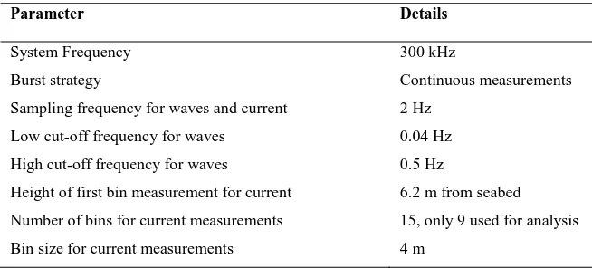
ADCPs rely on the principle of “Doppler shift” of the acoustic signals reflected off tiny particles to get an estimate of the water velocity. With an ADCP, the water column is discretised into a number of bins at the centres of which current velocities are estimated, resulting in a vertical velocity profile. The 300 kHz ADCP was deployed on the sea floor in a purpose-built mooring frame, looking upwards in a mean water depth of 40m. Single ping measurements were used in order to reduce bias in the turbulence measurements (i.e. reduced temporal resolution) as opposed to averaged sub-pings, e.g. mode 12 used with RDI ADCPs. The main deployment parameters for waves and currents are summarised in Table 1. An illustration of the 5-beam ADCP, including a definition of the axis system and geometrical angles, is shown in Fig. 3.

Compared with the standard 4-beam “Janus” configuration, the present 5-beam ADCP has an additional vertical 5th beam, used for high resolution direct surface tracking of the waves. The four inclined beams perform two functions: 1) estimation of directional wave spectra from the wave-induced orbital velocities, and 2) measurement of the along-beam current velocity throughout the water column. The uniform bin size used by the inclined beams was 4m, which is large but this was set to force low variance orbital velocities for accurate estimates of directional wave spectra [17]. Unfortunately, this also fixed the bin size for current measurements to 4m, from which turbulence metrics were derived. In comparison, it is customary to use small bins of 0.5 to 1.0 m for current measurements but at the time of the field study the ADCP could not be set up with different bin sizes for waves and currents. In terms of the focus of the paper, this setup is likely to limit the turbulent spatial scales that can be resolved from current measurements. It can be argued, however, that quantities such as Reynolds stresses and turbulent kinetic energy (TKE) mainly depend on the large scales of the flow [18] and as such may not require the smallest scales to be resolved. Available ADCP types cannot accurately measure turbulence quantities that depend on the smallest scales of the flow. To fully resolve such scales, it is required that the sensing volume is smaller than the smallest scales of the flow [19, 20]. In addition to the spatial scales, the 2 Hz sampling frequency used by the ADCP means that the time scales that can be resolved are limited to 1 Hz.

4

control procedures (performed in Matlab) were applied to the time series of current velocity in order to remove outliers such as bad data and erroneous spikes. Spline interpolation was used to replace missing data (typically < 1%). The aim of these quality control measures was to reduce bias in the computation of turbulence metrics. The instantaneous along-beam current velocities can be transformed into the Cartesian (Earth) system of velocities (u, v, w) where the directions of horizontal velocities u and v and vertical component w are positive to the East, North, and upwards, respectively (see Fig. 3). These velocities represent the dominant modes of motion. To avoid transducer ringing effects [17], the first measureable height for current velocities was at 6.2 m from seabed. Clearly, this was done at the cost of not sampling the part of the flow closer to the bottom boundary layer where shear stress and sediment transport processes are particularly important.

Each pair of opposing inclined beams resolves a horizontal velocity and the vertical component w. By reference to Fig. 3, the pair of beams 1 and 2 resolve for u and w while beams 3 and 4 resolve for v

and w. The pitch, roll, and yaw angles φ1, φ2 and φ3are important when considering the errors

introduced due to ADCP tilt, as discussed in Section 6.

3.

Mean flow and turbulence parameters

3.1

Mean flow

Due to the random nature of turbulence, statistical descriptors are usually based on velocity time series similar to what is collected here by the ADCP. Each instantaneous velocity component is decomposed into a mean and a fluctuating part such that for the u velocity

u u u' (1)

the bar indicates a time- averaged quantity (or mean) while the prime is the fluctuating velocity with zero mean. The fluctuating velocity components

u'

,

v'

, and

w'

as measured by the inclined ADCP beams may in practice include contributions from tangential wind stress, internal wave breaking, currents and other surface wave-related events e.g. orbital velocities, wave breaking and Langmuir circulation. The largest influences on the velocity current perturbations usually come from the orbital velocities. However, the data set collected during the study period shows no discernible interaction of the waves with the tidal currents (see Colucci et al. [14, 15]) meaning that the turbulence metrics presented can be considered to experience limited wave effects. The range of motions that are excited in the ocean due to large Reynolds number flows contributes to the patchiness (in space) and intermittency (in time) of turbulence, making it extremely difficult to separate the sources of turbulence in field measurements [21]. For instance, the distinction between velocities due to the background current and those due to the waves are important in situations where one is interested in the dynamic effects of wave current interactions. In such a case, it is possible to use linear wave theory to estimate the Stokes drift due to the waves. Fig. 4 illustrates the variation of the Stokes drift along the water column during a high water condition (low current speeds), showing that the effects of waves on the mean current velocity are minimal, diminishing quite rapidly with depth. Despite being small, the Stokes drift is removed from the mean current speeds. It is noted that measurements of the orbital velocities by the ADCP are taken at three bin heights only, few meters below the upper surface for the purposes of estimating directional wave spectra.

Soulsby et al. [22] suggested that a suitable averaging time is in the range of 8-12 minutes for tidal flows. In this study, 10 minute time-averaged velocities were used to investigate the nature of the mean flow. The averaging period is sufficiently long to provide a good sample of the largest turbulent eddies, but not so long that the turbulent processes cannot be considered as quasi stationary [23]. It is noted that depending on the quantity being investigated, either along-beam velocities (bi in Fig. 3) or

5

3.2

Turbulence intensity

Turbulence intensity is a measure of the size of the turbulent fluctuations and is therefore crucial in field investigations. The level of turbulence intensity can influence the loadings experienced by the blades of tidal stream turbines [1]. Turbulence intensity is a widely used parameter in the wind industry [6], but may also be used to characterise tidal energy sites. It is defined as the standard deviation of velocity fluctuations to the mean. For the u component, a turbulent intensity Iu may be

defined as

 

u

t ' u u I

2 u

u 



 (2)

where in the usual notation, the bar indicates a time average, and σu is the standard deviation of the

velocity fluctuations of u (here taken as the RMS value). Turbulent intensities for v and w, i.e. Iv and

Iw, are defined in a similar way to equation (2). Turbulence intensity is often reported in field studies

focused on marine energy (e.g. Milne et al. [5], Thompson et al. [6]). Many commercial codes such as Fluent and hydrostatic models that are used to model tidal turbines require, as input, measured values for turbulence intensity.

3.3

Reynolds stresses and TKE

Field measurements of Reynolds stresses in ocean flows can be used to assess the turbulence closure models since implementation of a closure model is a major source of uncertainty in oceanographic and hydrodynamic modelling [24]. Because the Reynolds stresses express the transport of momentum by turbulence, they control the vertical structure of turbulent flows. One of the practical uses of measuring Reynolds stresses is for estimating the eddy viscosity that is often used to describe vertical mixing due to turbulence [3]. Estimates of the Reynolds stresses are obtained using the along-beam velocities within the framework of the variance method, as originally proposed by Lohrmann et al. [25] and further extended by Stacey et al. [26], Lu and Lueck [27], and Williams and Simpson [28]. The variance technique has been used to estimate values of Reynolds stresses and turbulent kinetic energy (TKE) at tidal energy sites, e.g. Osalusi et al. [3], Togneri and Masters [29]. The variance method is popular in use because it gives reliable estimates in sites with strong currents as demonstrated in the literature (e.g. [3], [20], [24]). Although this means that the technique may be less accurate in wave dominated environments, the Wave Hub site has moderately strong currents and so the variance method is applicable. The basis of the variance method is as follows. First, each inclined beam (labelled i = 1, 2, 3, 4) returns time series of the current velocity along its axis, i.e. velocity bi. The pairs of opposing beams (1 & 2) and (3 & 4) lie in two perpendicular planes x-z and

y-z, respectively. The total current velocity is then assumed to be homogeneous across the horizontal distance of each opposing beam pair, so that the statistics of turbulence are the same for the four beams [27]. This means that the second order moments of fluctuating velocities are also horizontally

homogeneous, i.e. ' 2 ' 2

1 2

u u , ' '

1 1

u w = ' '

2 2

u w , etc. In addition to the horizontal homogeneity assumption, flow stationarity is satisfied when an appropriate averaging time period, here 10 minutes, is used [23]. Of course, ocean turbulence is unlikely to be stationary, homogeneous or isotropic because of the effects of shear, stratification, presence of boundaries and high Reynolds numbers [21]. Assuming the ADCP sits flat on the seabed with zero tilt, geometrical considerations result in two components of the Reynolds stresses that relate the velocity variances of the along-beam velocities with those in the Cartesian coordinate, as in equation (3)

 

 



2 sin 2 ' '

2 ' 1 2 '

2 b

b w u

x    _,

 

 



2 sin 2 ' '

2 ' 3 2 '

4 b

b w v

y _{ } 

(3)

where ' 2 i

6

the vertical (Fig. 3), and ρ is the water density. From the definitions of the Reynolds stresses in equation (3), these increase with increases in fluctuations, i.e. with turbulence intensity. Our sampling strategy which uses individual velocity pings to calculate turbulent parameters ensures that the Reynolds stresses are not underestimated, in contrast to other approaches where significant loss of variance may occur due to the along-beam velocities being obtained from averaging a number of pings (e.g. a 23% underestimation of Reynolds stresses was reported in [23]); this was done primarily to achieve extended periods of data recording. Equation (3) also means that when using the variance method with ADCPs it is not possible to get the Reynolds stresses directly. In contrast, when using ADVs with high frequency sampling over a small water volume, one is able to get direct

measurements of quantities e.g. ' '

u w from the covariance of u and w [30].

The profiles of TKE cannot be computed from ADCP data without a further assumption to that of horizontal homogeneous flow between opposing beams. Lu and Lueck [27] defined a quantity S

which is related to the TKE density via a turbulence anisotropy ratio α, such that

 

' 2 ' 2 ' 2 ' 2 2

1 2 3 4

2 2

b b b b 1 2 q

S 1

1 2

4 sin tan

 

 

 

    

  _  _{ } 

  _{ } (4)

The anisotropy ratio α is defined as

2 2 2

w' / u' v'

  _  _

  (5)

while the profiles of TKE density are defined in the usual way as

2 2 2 2

q / 2_u' v' w' _/ 2

  (6)

In this study, a value of α = 0.17 was assumed based on measurements from an unstratified open tidal channel [26], and based on the argument that

2 2 2

w' _u' v' _/ 2

  (7)

as originally postulated by Lohrmann [25]. In fact, this value of α has been used by other researchers (e.g. Osalusi et al. [3], Williams et al. [28] and Togneri and Masters [29]) and is considered a reasonable approximation for a wide range of turbulent flows in open channels and in the ocean. With

α = 0.17, equation (4) gives S = 3.05 q2/2. Within the context of the distribution of TKE in a water column, field investigations of turbulence enable the use of TKE data to understand the mechanism of wave energy dissipation when wave or tidal energy converters are deployed on site.

3.4

Integral scales

The integral time scale defines the time period during which the largest eddies of the flow are correlated and represents the largest scales in the energy spectrum. The turbulent eddies are generated as a result of instabilities induced by the shearing of the mean flow, which are then dissipated through viscous effects [31]. The eddy size specifies the typical flow structures marine energy devices interact with at sea. The integral time scale Ti for a sample of measurements can be expressed as

 

0

i ii

0

T R d





  





_,

 



  





2 ' , '

u uu

t u t u R R





7

where Ruu (τ) is the autocorrelation function for velocity fluctuations 'u and τ0 is the instance when Ruu becomes zero. Estimation of autocorrelation requires a continuous time series of velocity

samples that are evenly spaced in time. In practice, the integral time scales are computed by summing the auto-correlation function over a sufficiently long time (e.g. here 200 seconds), or by using the upper time limit where Rii = 0. To calculate the integral length scale Li, Taylor’s hypothesis of frozen

turbulence is invoked such that Li = Ti Ui where Ui is the mean of the along-beam velocity. Thus,

integral length scales from the along-beam velocities of each inclined beam can be defined. Another way of estimating length scales was defined by Dillon [32] who proposed a mixing length scale lm

1 2

m

u' w' l

u z

 



 

 _{ } _ 

 

(9)

When estimating the integral length scales, these should be sufficiently large compared with the

vertical height of the bins. Since the mixing length scale depends on the vertical velocity shear z u

  _{, it}

clearly requires sufficiently small bins for accurate estimations. In open channel flows, Stacey et al. [26] commented that the length scales of turbulence would be expected to vary parabolically in relation to the water depth. Although flows in the open sea are not directly comparable to open channel flows, the theoretical parabola profile provides a useful reference for comparison. Thus, it is plotted along with the other profiles as discussed in Section 4.

4.

Results

The turbulence parameters estimated in this paper are those likely to affect the operational performance of wave and tidal energy converters. As mentioned in Section 3.1, the metrics have limited wave effects since there is very little interaction between the waves and currents at the site as demonstrated in Colucci et al. [15, 16]. Part of the analysis will consider flow states near the spring and neap tides, to allow for some cross comparisons. Also for presentation purposes, the mean and turbulent flow characteristics are considered separately.

4.1 Mean flow characteristics

Fig. 5 shows the variation of the magnitude of the mean current velocity vector during the deployment period, illustrating a degree of bi-directionality between ebb and flood. There is, however, slightly more directional scatter for flood velocity compared with ebb velocity. For both ebb and flood, there is slightly more directional spread at slower velocities. The mean directions from North are 248° and 66° for flood and ebb, respectively. In practice, knowledge of the magnitude and direction of ebb and flood helps device developers to understand the possible impact of ocean currents on the hydrodynamics of wave energy devices, especially when the currents interact with strong waves. For instance, some aspects of wave-current interactions and their influence on the quantification of the tidal energy resource have been discussed by Lewis et al. [11].

8

velocity component was the largest followed by v, although both the v and w components were comparatively of much smaller magnitudes compared with u. A close up of a sample of current velocities is shown in Fig. 7 (with error bars) for successive tidal cycles near the spring tide: the flood velocities appear to be only slightly greater than the ebb. The results in Figs. 6 and 7 reiterate the advantage of using ADCPs to obtain profiles of current velocities with water depth in a relatively deep site.

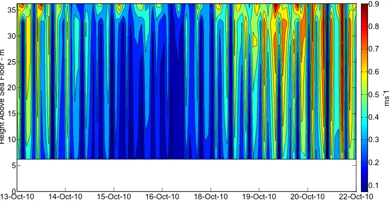
Time series of the contours of mean velocity profiles during the full deployment are shown in Fig. 8, illustrating how the magnitude of the total current speed increases, as expected, with height above seabed. Selected profiles of mean current over a tidal cycle are illustrated in Fig. 9 comparing one case near the neap tide with another during the spring tide. From Fig. 9, it is evident that while the qualitative shapes of the profiles remain nearly the same during all phases of the tide (whether neap or spring), the flood and ebb current magnitudes near the spring tide are larger than their values during the neap tide. For instance, the peak flood velocities at spring tide are three times larger than the corresponding values at neap tide (0.92 m/s and 0.29 m/s, respectively), while the peak ebb velocities during spring are as twice as large the ebb velocities at neap tide (0.83 m/s and 0.41 m/s, respectively).

However, the current magnitudes during high and low waters are similar for both tidal regimes. It is worth noting that for all profiles shown in this study, only nine bins are plotted. As recommended by ADCP manufacturers, the measurements should not be performed within the region of a few meters from the top surface to avoid contaminations due to the ADCP’s side lobe interference [17]. This choice is justified since beyond the ninth bin sudden increases in the magnitude of parameters were observed, indicating unrealistic behaviour.

Throughout the profiles, the current magnitude for flood is greater than that during ebb by approximately 0.1 m/s. There is also a greater reduction in velocity with depth during ebb compared with the flood tide. A similar observation was reported by Sutherland et al. [4] at a tidal channel which was attributed to local bathymetric variations. It is fairly common for tidal currents to be asymmetrical; for physical explanations see the studies by Neill et al. [33, 34]. The profiles of mean velocity during low and high waters are quite similar, but with slightly higher velocities during low water (a difference of about 0.03 m/s), especially nearer the top surface. At times when the peak tidal currents reach ~ 1m/s the water column is expected to be well mixed in the vertical direction. In general, there is some shear in the velocity profiles, which is not unusual for turbulent flows in oceanic environments.

4.2 Turbulent flow characteristics

In this part, the parameters of turbulence intensity, Reynolds stresses, turbulent kinetic energy, and the integral scales are estimated. Unlike the situation with the mean flow, the computation of these turbulence metrics requires the along-beam velocity fluctuations. Since the ADCP samples at 2Hz, velocity power spectra are not reported due to the limitation on the highest frequency resolved by the ADCP (1 Hz in our case): only a small part of the velocity spectra can be seen at low frequencies before measurements are quickly smeared by Doppler noise, making the measurements impractical.

4.2.1 Turbulence intensity

9

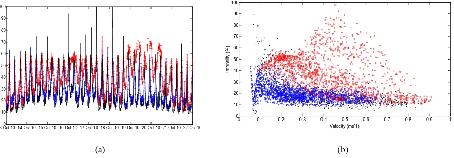
is much more erratic, with values of 70% being estimated at all current speeds. For the bin closest to the bottom (6.2 m above seabed), however, the turbulence intensity reduces to around 12-13 % at a mean velocity of 0.8 m/s.

Table 2 compares turbulence intensities (TI) obtained at a number of tidal energy sites with values computed at the mixed Wave Hub site. The mean velocity at which the turbulence intensity was estimated is shown in brackets. Comparisons between various tidal energy sites and between tidal and wave dominated sites such as the one shown in Table 2 are scarce. For the mixed Wave Hub site the turbulence intensity of the u component is the largest, the turbulence intensity of v has values of approximately 0.6-0.7 of u, while that of the vertical w component is approximately 0.2 times the u

component. Taking into account the effect of noise factor due to the angle of the beams from the vertical, the turbulence ratio is 1: 0.7: 0.55 between u, v and w respectively.

4.2.2 Reynolds stresses

Fig. 11 shows the profiles of Reynolds stresses u' w' and v' w' as they vary over a tidal cycle for neap and spring tides. The first observation is the increase in shear during the spring tide compared with the neap tide. The profiles in Fig. 11 show generally that the magnitude of Reynolds stress may increase or decrease away from the seabed depending on the phase of the tide. For the u' w'

component, the general trend for all phases of the tide a decrease in the stress over the bottom half of the water column and an increase thereafter. The opposite is true for the v' w' component. From Fig. 11, the two components of Reynolds stress are thus opposite and symmetrical about each other over a tidal cycle especially within a neap tide. But such symmetry is less pronounced for the tidal cycle near the spring tide. The phases of the tide seem therefore to have less of an effect on the Reynolds stress values than where within the spring/neap cycle the tide is. In the study of Osalusi et al. [3], the authors reported that asymmetric profiles were observed in the Reynolds stresses between ebb and flood for a fast flowing flow in a tidal channel, for all tidal phases. This may turn out to be one of the key differences between flows at tidal channels and those at mixed wave sites. Despite the similarity in asymmetric profiles that are consistent with the observations of Osalusi et al. [3], it is not yet clear why the Reynolds stress profiles during the spring tide are different from those during the neap tide. Possible reasons may include errors in velocity measurements or that during the spring tide there could have been some strong wave breaking from the top surface as well as internal wave breaking, resulting in increased momentum diffusion that breaks the symmetry of the profiles.

4.2.3 Turbulent kinetic energy (TKE)

10

4.2.4 Integral scales

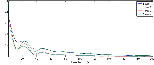
In Fig. 13, samples of auto-correlation functions computed from the along-beam velocities are plotted, showing some oscillations at lower time lags. Some degree of periodicity in the flow may therefore exist. The integral time scales were studied for tidal cycles at both neap and spring tides. For a period of 8.5 hours, the largest time scales were found in the region of 20-25 seconds during spring tides and 10-15 seconds during neaps. Thus, over the sampling period in the region of 1000-1500 large scale turbulent flow structures were sampled. The larger time scales also mean larger length scales during the spring tide compared with the neap tide. It is suggested that this discrepancy may be the result of the flow during the spring tide being more turbulent, thereby creating larger turbulent eddies. A similar observation was reported by Togneri and Masters [35] for a tidal channel. In Fig. 14, the length scales from the four inclined beams generally produce qualitatively similar shapes. Also, for each pair of opposing beams (pair 1 & 2 or pair 3 & 4) similar qualitative shapes of the length scales are observed.

Despite the large bin size of 4m, the integral length scales show a good level of correlation with the shape and magnitude of the mixing length scale. The integral length scales calculated for beams 3 and 4 match the estimated mixing length scales especially well. Another observation is that the length scales calculated for beams 1 and 2 are significantly larger than for beams 3 and 4. Particularly during spring tides, the length scales appear to be nearly twice as large as those along beams 3 and 4. One possible explanation for this discrepancy is that the flow in the x-z plane of beams 1 and 2 (with the largest u component) produces larger turbulent structures and thus results in larger time and length scales. However, further measurements are needed to explain such discrepancy.

5.

Error Analysis

Some discussion of the errors involved in the estimation of turbulence metrics is presented next.

5.1 Errors due to the homogeneity assumption

In a turbulent flow, the instantaneous velocities measured in one beam will be different from those in another beam [20]. The horizontal distance d between opposite beams (see Fig. 3) as given by

d = 2zsinθ, where z is the vertical distance above the ADCP, shows that the further from the ADCP that the measurements are taken the greater the beam spread will be. What this means in practice is that flow dynamics changing on a length scale smaller than twice the beam spread are not likely to be resolved [36]. Applying this to the case of ADCP field measurements for current marine turbines (e.g. at 20 m from seabed), the resolved eddies are of most practical use when their size is comparable to the length of the turbine blades. Beam spread itself is constrained by ADCP configuration (i.e. beam angle), bin size, system frequency, and water depth. With large beam spread, there is always less confidence in the resolved (u, v, w) velocities away from the seabed. Thus, one must appreciate that the homogeneity assumption for instantaneous currents becomes increasingly less applicable as d

11

5.2 Errors due to equipment tilt

The accuracy of the variance method is affected by the amount of pitch and roll that may occur during deployment. In our case, the pitch and roll angles were 3.5° and 5°, respectively. Because the ADCP was rigidly mounted, the angles of pitch and roll were constant throughout the deployment, meaning the ADCP did not undergo any appreciable dynamic motions. If zero tilt can be achieved (i.e. the ADCP completely flat on the sea floor), it turns out that the Reynolds stresses can be calculated without further approximations [38]. If there is a non-zero tilt, however, extra terms are introduced into the estimates of Reynolds stresses and TKE, thus introducing some bias. Because the tilt and roll angles are small (≤ 5°), small angle approximation leads to sin φ ~ φ and cos φ ~ 1. Then, the equations for calculating the Reynolds stresses with non-zero tilt can be estimated as [38]:

 

' 2 ' 2

2 2

2 1

3 2

b b

u' w' u' w' u' v'

2 sin 2  

  

   _  _ 

  (10)

 

' 2 ' 2

2 2

4 3

2 3

b b

v' w' v' w' u' v'

2 sin 2  

  

   _  _ 

  (11)

Dewey and Stringer [38] showed that equations (10) and (11) can be re-arranged to yield

 

' 2 ' 2

' 2 ' 2 2 3

2 1

2 1 2

2

b b 1

u' w' b b w' u' v'

2 sin 2 sin 2

 _

 

    

   _{ }  _ _

 

  (12)

 

' 2 ' 2

' 2 ' 2 2

4 3 2

4 3 3

2

b b 1

v' w' b b w' u' v'

2 sin 2 sin 2

 _

 

    

   _{ }  _ _

 

  (13)

But there are still two unknowns, w'2 and u' v' that cannot be derived from the measured ADCP data. However, it was shown in [38] that these terms are small and may be ignored for initial estimates. This leaves the second term in equations (12) and (13) which contributes to bias. Summaries of the effect of the tilt angles on the statistics of the Reynolds stresses are shown in Tables 3 and 4. It is clear that the estimates are quite sensitive to even small values of roll and pitch angles. The main thing, nonetheless, is the ability to correct for these uncertainties as long as the angles remain small. In this case, users of this data should use the values of Reynolds stresses obtained after the tilt corrections. In the study by Lu and Lueck [27], it was shown that a 2° tilt resulted in about 17% bias in the estimates of the Reynolds stresses. This illustrates the sensitivity of Reynolds stress measurements to ADCP tilt. One solution to minimise ADCP tilt is to use a gimbal on the deployment frame to adjust for uneven surfaces; a similar approach was used by Osalusi et al. [3] during field measurements at a tidal energy site.

5.3 Doppler noise

12

high frequency inertial subrange of turbulence in a tidal channel [9]. For the ADCP, each beam measurement contains an error such that b*i = bi + N, where b*i is the measured velocity, bi is the

actual current velocity, and N is a random variable associated with Doppler noise. ADCP Doppler noise originates from errors associated with the Doppler shift of the reflected acoustic signal [20]. Such errors may themselves be caused by variations of sound scattering off particles in the water flow [42]. Nystrom et al. [20] provide a good discussion on the factors that may contribute to Doppler noise. Two types of uncertainty result from Doppler noise: bias and spread. Bias shifts the measured data away from the true values and will not be reduced by data averaging, whereas spread causes a widening of the distribution of the data points and can be reduced by averaging. Stacey et al. [26] showed that the Reynolds stress calculations do not suffer from bias, the estimation of the TKE does, however. By a histogram of the values of S (not shown), it was found that there are no values of S

that are < 3.16 x 10-3 m2s-2. This value is removed from the estimates of S before calculating a final value for the TKE. The value of the noise variance corresponds to an error of 5.62 x 10-2 ms-1 per ping. The amount of Doppler noise removed from the estimates of Reynolds stresses in this paper was chosen according to the recommendations of RDI’s PlanADCP software [17]. The turbulence intensity is also corrected for Doppler noise such that a corrected version of equation (2) is used [6]

 

u

n t ' u I

2 2

corrected , u



 (14)

where n here is the estimated Doppler noise as specified by RDI during the configuration setup of the ADCP. Although Williams and Simpson [28] reported that RDI’s PlanADCP values may be biased low, not accounting for Doppler noise at all means unnecessarily high factors of safety for marine component designs, because the resulting turbulence intensities would be biased high [6]. One possible approach to reduce noise in future measurements would be to utilise fast pinging modes, with averaged sub-pings. This approach was previously reported to offer lower measurement uncertainty in contrast to a mode based on single pings [41]. However, averaging via sub-pings must not lead to filtering out the significant energy containing scales from the velocity measurements [41].

6.

Discussion

Clearly, with higher bin resolution (typically 0.5m or 1m) it would be possible to define more accurately the vertical shear variation du/dz of the velocity profiles. In practice, sheared velocity profiles can affect the performance of marine energy systems including the amount of power extracted, as discussed by Mason-Jones et al. [43]. With a single ADCP it was only possible to optimise it for one measurement: waves in this case. While the results obtained are limited due to using 4m bins, large bin size should not stop researchers from maximising the use of their data knowing that field measurements are quite expensive and challenging to undertake, and with high levels of risk. With higher bin resolution, one would have more information regarding the type of mathematical profiles that can be used to describe the velocity profiles e.g. a log-law or power law profile. For the jumps observed closer to the top surface, it is likely that the ADCP is not able to produce accurate measurements of current data due to side lobe interference effects [17].

13

these times there would not be sufficient flow to operate current turbines. It is indicated from Fig. 10 that closer to the surface there seems to be a different turbulence level, possibly driven by near surface effects such as wave breaking and wind stress. Results of turbulence intensity from the first bin are the closest data to use for comparison. At a height of 5m in the tidal energy site at the Sound of Islay, UK [5] the authors reported turbulence intensities of 13% at flood tide and 12% during ebb, over a tidal cycle that excluded periods of slack water. Similar levels of turbulence intensity were reported by Thomson et al. [6] at 4.6m from seabed. In comparison with this study, the differences seen at the tidal sites may be due to the mean current velocity in those locations being slightly higher than at the Wave Hub site. This may also indicate that turbulence intensity is site specific as suggested by Milne et al. [5] and Okorie & Owen [44]. The turbulence intensity ratio of 1: 0.7: 0.55 reported here compares with the ratio of 1: 0.75: 0.56 obtained by Milne et al. [5] for a tidal site, and with that of 1:0.71:0.55 as computed by Nezu and Nakagawa [45] for an open channel (all these ratios were obtained at approximately 5m above seabed). Although no observation of turbulence in the ocean can be considered typical [21], the comparison of the turbulence ratios between independent sites and the good agreement observed may indicate that there are some typical characteristics of tidal currents that are consistent even in active wave sites. Normally, one would expect the ratio of v:u as discussed here to be a function of the flow direction which is site specific. Fair comparisons between independent sites could be used to define general guidelines on the properties of marine energy sites.

The difference in the Reynolds stresses observed between the neap and spring tides (Fig. 10) may be associated with higher velocities during spring tide which induce higher momentum exchange over the water column, leading to higher shear. The increase in activity for theu' w' component during the deceleration phase of the tide as in Fig. 10 (a) was also reported in the study by Stacey et al. [26] in an energetic tidal channel. The sudden changes seen in the Reynolds stresses near the free surface may be attributed, in part, to the wave-induced orbital velocities. The straining by the wave orbital velocities on the shear stresses near the top surface was demonstrated by Teixeira and Belcher [46] who studied the dynamics of upper ocean turbulence interacting with surface waves. The reduced symmetry of Reynolds stresses for the spring tide might be the consequence of increased shear in the stress profiles because of higher flow velocities; the increased shear makes it difficult to sustain flow symmetry. The Reynolds stresses obtained from single ping measurements as in the present study may be overestimated, though this effect is less significant compared with the case of more energetic tidal flows [41].

Regarding the periodicity of autocorrelations seen at low frequency flow oscillations, this was also reported in the field measurements of Milne et al. [5] in a tidal channel. The difference in beam length scales is most significant towards the bottom of the water column. Near the free surface, however, the beams exhibit similar profiles despite the beam spreading becoming greater. Although causes of these trends remain unclear, they seem to be a consistent behaviour of integral length scales along a full water column. For beams 1 and 2 at 6.2 m above seabed, their length scales are respectively 15m and 9.8m at neap tides and 25m and 19.5m during spring tides. In the study of Milne et al. [5], length scales of 11.3m were reported during the ebb phase of the tide for measurements at 5m above seabed in a tidal channel of 55 m mean water depth. Thus, there is a relatively close agreement with the present field measurements. Despite the fact that similar length scales (of the mixing type) were reported by Togneri and Masters [35] at tidal sites with comparable water depths to the Wave Hub, the same authors also reported much lower length scales for shallower locations (length scales of approximately 3m maximum in water depths of less than 20m). This means that such trends in length scales may be dependent on the mean water depth.

7.

Conclusions and future work

14

limited effects from the waves. Constrained by an optimised setup for wave measurements, this paper has investigated typical turbulence characteristics at the site using secondary current velocity data as measured by the ADCP’s inclined beams. Results presented in this paper suggest that it is possible to use a non-optimum ADCP setup to derive typical characteristics of field turbulence in a mixed, low tidal energy site. It is found that the currents at the site are tidally driven, the ebb and flood are nearly bi-directional, and the maximum current speed is approximately 1 m/s with 4-5m tidal level variation. For the mean flow, the horizontal u and v velocity components are much larger than the vertical velocity w, with the v component being almost half of the u component. The mean velocity profiles have some shear and increase, as expected, with water height above the sea floor. The turbulence intensity varies between flood and ebb, but is no less than 10% at peak speeds. Although some of the reported turbulence intensities are comparable to those estimated at tidal energy sites (at ~ 5m above seabed), the study also shows that turbulence intensity might be site specific. The turbulence ratio is typically 1: 0.7: 0.55 between u, v and w respectively, which is similar to turbulence ratios estimated elsewhere at similar heights above the seabed. While symmetry between the Reynolds stress components u' w' and v' w' is clearly observed over consecutive tidal cycles of the neap tide, such symmetry is less apparent for tidal cycles near the spring tide. The phases of the tide seem to have less of an effect on the Reynolds stress values than where within the spring/neap cycle the tide is. Assuming an anisotropy ratio based on channel flows, the profiles of TKE are shown to follow expected trends, increasing with height above the seabed. However, the values of TKE are larger during the spring tide compared with a neap tide. Throughout the deployment, it is also found that the TKE values of the ebb flow are the largest. The along-beam integral length scales have been estimated and compare favourably to integral scales from other tidal sites at about 5m above sea floor. Qualitatively, they also compare favourably to theoretical profiles and the mixing length scale. An error analysis reveals that users of the data should be aware of the bias in the estimated parameters especially that due to ADCP tilt, Doppler noise, and flow inhomogeneity. The Reynolds stress estimates are particularly sensitive to tilt angles, and can be corrected for small roll and yaw deviations. Despite the limitations of the ADCP setup, estimation of some turbulence metrics is useful and has revealed interesting trends for the currents at the mixed site and in comparison with estimates at other tidal energy sites. Because sea deployments are very expensive and data on field turbulence is difficult to obtain, this paper contributes to the growing number of field studies at marine energy sites and demonstrates the practical benefit of secondary data even when the ADCP is not optimised for turbulence measurement. Through further analysis of currents, it is clear that tidal currents in mixed sites exhibit characteristics that are sometimes similar to those at tidal channels but may have their own characteristics. Developers of wave and tidal energy converters can use such turbulence data to assess the impact of the flow on the unsteady loading experienced by offshore devices, at least in terms of the largest scales.

While it is possible to use an ADCP to measure both waves and currents, it remains difficult to optimise the unit to measure both flows accurately in a single deployment. For the 5-beam ADCP with a sampling rate of 2 Hz, if one is interested in waves then the vertical beam should be used for direct surface tracking to estimate the non-directional waves, while the inclined beams estimate the directional wave information using large, low velocity variance bins. The result is a compromise on the spatial resolution available to characterise the turbulence from the current data, as demonstrated in this paper. If, however, the setup is optimised for measuring currents, the vertical beam could be used to provide direct estimates of the vertical velocity, while the inclined beams provide measurements for the u and v velocity components, in addition to directional wave information. The downside of the latter setup is that existing ADCPs cannot offer direct surface tracking capability to characterise the waves, while the use of smaller ADCP bins for current measurements would return noisier signals. However, in either case above, users can benefit from the secondary data, whether waves or currents, to maximise the benefit of expensive and challenging field measurements.

15

turbulence metrics (or even on wave information) can be undertaken. It is also desirable to test the ability of the vertical beam to measure the vertical velocity w directly. This would partly relax the assumption of flow inhomogeneity, improve estimates of higher moment statistics, and generally provide more accurate estimates of Reynolds stresses and TKE. In the future, researchers would want to use smart combinations of wave and current measurement sensors, so that in addition to wave data, high frequency, high quality current data can return reliable turbulence estimates. This can be achieved using high frequency ADVs co-located with wave buoys, or with ADCPs equipped with vertical beams. Sensors with high frequency sampling (e.g. 10-20 Hz) would allow users to obtain velocity power spectra which contain detailed information about the range of turbulent eddies. Other options include developing low power, low cost Autonomous Underwater Vehicles (AUV) that can provide higher sampling frequencies and extended periods of measurements.

Acknowledgments

The authors would like to thank Prof. George Smith for his tireless enthusiasm that underpins the research carried out within this group, built and guided by his knowledge and expertise. He is greatly missed. Brandon Strong of Teledyne RDI has provided practical tips on the processing and use of the ADCP. Two anonymous reviewers provided constructive comments and suggestions. This research uses fieldwork carried out through the EDF funded PRIMaRE and MERiFIC projects, and this support is gratefully acknowledged. The authors would also like to acknowledge the support of the TSB through the ‘High Flow Installation Vessel’ project (Ref: 101315).

References

[1] I. A. Milne, R. Sharma, R. G. J. Flay, and S. Bickerton, “The role of onset turbulence on tidal turbine blade loads,” in Proc. 17th

Australasian Fluid Mechanics Conference, 2010, Auckland, New Zealand.

[2] G. March, “Wave and tidal power- an emerging new market for composites,” Reinforced Plastics., vol. 53, pp. 20–24, 2009.

[3] E. Osalusi, J. Side, R. Harris, 2009: Structure of turbulent flow in EMEC's tidal energy test site. International Communications in

Heat and Mass Transfer 36 p422-431l.

[4] D.R.J. Sutherland, B.G. Sellar, I. Bryden, “The use of Doppler sensor arrays to characterize turbulence at tidal energy sites”, In

Proceeding of the 4th _{International Conference on Ocean Energy, Dublin, 2012.}

[5] I. A. Milne, R. Sharma, R. G. J. Flay, and S. Bickerton, “Characteristics of the turbulence in the flow at a tidal stream power site”,

Phil. Trans. R. Soc. A., vol. 371, pp.1-14, January 2013.

[6] J. Thomson, B. Polagye, V. Durgesh, M. C. Richmond, 2012: Measurements of Turbulence at Two Tidal Energy Sites in Puget

Sound, WA, Journal of Oceanic Engineering, Vol 37, issue 3, p363-374.

[7] Y. Li, J.A. Colby, N. Kelley, R. Thresher, B. Jonkman, S. Hughes, “Inflow measurement in a tidal strait for developing tidal current

turbines: lessons, opportunities and challenges”, In Proceedings of ASME 2010, 29th _{International Conference on Ocean, Offshore}

and Arctic Engineering (OMAE2010), Shanghai, China, 6-11 June 2010, vol. 3, pp.569-576, New York, NY: American Society of Mechanical Engineers.

[8] Gunawan, B. Neary, V., and Colby, J. Tidal energy site resource assessment in the East River, NY (USA). Renewable Energy,

submitted, 2013.

[9] Jean-Baptiste Richard, J. Thomson, B. Polagye, J. Bard, “Method for Identification of Doppler Noise Levels in Turbulent Flow

Measurements Dedicated to Tidal Energy”, 10th _{European Wave and Tidal Energy Conference, Aalborg, Denmark, 2-5 Sep 2013.}

[10] Hashemi, M. R., Neill, S. P., Robins, P. E., Davies, A. G., and Lewis, M. J. Effect of waves on the tidal energy resource at a planned

tidal stream array. Renewable Energy 75, 626-639, 2015.

[11] Lewis, M.J., Neill, S.P. and Hashemi, M.R. Realistic wave conditions and their influence on quantifying the tidal stream energy

resource. Applied Energy 136, 495-508, 2014.

[12] Smith HCM, Haverson D, Smith GH, Cornish CS, Baldock D. Assessment of the wave and current resource at the Wave Hub.

Proceedings of the 30th _{International Conference on Ocean, Offshore and Arctic Engineering 2011; June 19-24, Rotterdam,}

Netherlands.

[13] B. Strong, A. Bouferrouk, and G.H. Smith, “Measurement and evaluation of the wave climate near the Wave Hub using a 5-beam

ADCP”, in Proc. ICOE, Dublin, October 2012.

[14] Saulnier JBMG, Maisondieu C, Ashton IGC, Smith GH. Wave Hub test facility: sea state directional analysis from an array of 4

measurement buoys. Proc. of 9th _{EWTEC 2011; Southampton, UK.}

[15] Colucci AM, Johanning L, Hardwick, JP. Investigating the interaction of waves and currents from ADCP field data, MTS/IEEE St.

John's Oceans: Where Challenge Becomes Opportunity, St. John's, Canada, 2014.

[16] Colucci, A., Bouferrouk, A., Hardwick, J. and Johanning, L. Characterising wave-current fields and their interaction from in situ

measurements. In: 10th European Wave and Tidal Energy Conference, Aalborg, Denmark, 2 - 5 September, 2013.

[17] RDI Primer

[18] P. Bradshaw, “An introduction to turbulence and its measurement”, Pergamon, Oxford, UK, 1971.

[19] J. O. Hinze, “Turbulence”, McGraw-Hill, New York, 1975.

[20] E. A. Nystrom, C. R. Rehmann, M. Asce, K. A. Oberg, “Evaluation of the mean velocity and turbulence measurements with ADCPs”,

Journal of Hydraulic Engineering, pp.1310-1318, 2007.

[21] J. N. Moum, and T. P. Rippeth, “Do observations adequately resolve the natural variability of oceanic turbulence?”, Journal of

Marine Systems, Volume 77, Issue 4, Pages 409–417, 2009.

[22] R. L.Soulsby, “Selecting record length and digitization rate for near-bed turbulence measurements”, J. Phys. Oceanogr., 10, 208–

16

[23] T.E. Faber, “Fluid Dynamics for physicists”, Cambridge University Press, 1995.

[24] T.P. Rippeth, J.H. Simpson, E. Williams, M.E. Inall, “Measurement of the rates of production and dissipation of turbulent kinetic

energy in an energetic tidal flow: Red Wharf Bay revisited”, Journal of Physical Oceanography, vol. 33 (9), pp.1889-1901, 2003.

[25] A. Lohrmann, B. Hackett, L.P. Roed, 1990: High resolution measurements of turbulence, velocity, and stress using a pulse-to-pulse

coherent sonar, J. Atmos. Ocean. Technol. 7, p19–37.

[26] M. T. Stacey, S. G. Monismith, and J. R. Burau, “Measurements of Reynolds stress profiles in unstratified tidal flow”, Journal of

Geophysical Research., vol. 104, pp. 10,933-10,949, May 1999.

[27] Y. Lu, and R. G. Lueck, “Using a broadband ADCP in a tidal channel. Part II: Turbulence”, J. Atmos. Ocean. Technol., vol 16 (11),

pp.1568-1579, 1999.

[28] Williams, J.H. Simpson, Uncertainties in estimates of Reynolds stress and TKE production rate using the ADCP variance method, J.

Atmos. Ocean. Technol. 21. pp. 347–357, 2004.

[29] M. Togneri, and I. Masters, “Comparison of turbulence characteristics for selected tidal stream power extraction sites”, in Proc. ICOE,

Dublin, October 2012.

[30] A. J. Souza, “The use of ADCPs to measure turbulence and SPM in shelf seas. 2nd International conference and exhibition on

Underwater Acoustic Measurements: technologies and results, 25-29 June 2007, Heraklion, Crete, 25-29 June 2007.

[31] Agrawal, Y. C., E. A. Terray, M. A. Donelan, P. A. Hwang, A. J. Williams, W. Drennan, K. Kahma, and S. Kitaigorodskii, 1992:

“Enhanced dissipation of kinetic energy beneath breaking waves”. Nature, 359, 219–220.

[32] T.M. Dillon, “Vertical overturns: A comparison of Thorpe and Ozmidov length scales”, Journal of Geophysical Research., vol 87

(C12), pp.9601-9613, 1982.

[33] Neill, S.P., Litt, E.J., Couch, S.J. and Davies, A.G. The impact of tidal stream turbines on large-scale sediment dynamics. Renewable

Energy 34 2803-2812, 2009.

[34] Neill, S.P., Hashemi, M.R. and Lewis, M.J. The role of tidal asymmetry in characterizing the tidal energy resource of Orkney.

Renewable Energy 68, 337-350, 2014.

[35] M. Togneri, and I. Masters, “Comparison of turbulence characteristics for selected tidal stream power extraction sites”, in Proc of the

2nd _{Oxford Tidal Energy Workshop, Oxford, 2013.}

[36] J. B. Richard, J. Bard, C. Rudolph, M. Milovich, “Assessing the capabilities of acoustic Doppler sensors for quantifying dynamic

phenomena in tidal streams”, 4th International Conference on Ocean Energy, 17th _{-19th October 2012, Dublin.}

[37] A. E. Gargett, “Observing turbulence with a modified ADCP”, J. Atmos. Ocean. Technol., vol 11, pp.1592-1610, 1994.

[38] R. Dewey, and S. Stringer, “Reynolds stresses and turbulent kinetic energy estimates from various ADCP beam configurations:

Theory”, Journal of Physical Oceanography., pp. 1-35, 2007.

[39] V. I. Nicora, and D. G. Goring, “ADV measurements of turbulence: Can we improve their interpretation?”, J. Hydraul. Eng., 124 (6),

pp. 630–634, 1998.

[40] S. Anderson, and A. Lohrmann, “Open water test of the Sontek acoustic Doppler velocimeter”, Proc., IEEE Fifth Working Conf. on

Current Measurements, IEEE Oceanic Engineering Society, St. Petersburg, Fla., 188–192, 1995.

[41] N.J. Nidzieko, D.A. Fong, J.L. Hench, “Comparison of Reynolds stress estimates derived from standard and fastping ADCPs”, J.

Atmos. Ocean. Technol., vol. 23, pp.854-861, 2006.

[42] SonTek, “Pulse coherent Doppler processing and the ADV correlation”, SonTek Tech. Note, San Diego, 1997.

[43] A. Mason-Jones, D. M. O'Doherty, C. E. Morris, T. O'Doherty, C. B. Byrne, P. W. Prickett, R. I. Grosvenor, S. Owen,

Ieuan and Tedds, R. J. Poole, “Non-dimensional scaling of tidal stream turbines”,Energy, vol 44 (1). pp. 820-829, 2012.

[44] P. O. Okorie, and A. Owen, "Turbulence: Characteristics and its implications in tidal current energy device testing," OCEANS, vol. 1,

no. 6, pp.15-18, Sept. 2008.

[45] I. Nezu., and H. Nakagawa, “Turbulence in open channel flows”, IAHR Monograph., Belkema, Rotterdam, Netherlands, 1993.

17

Tables

Parameter Details

System Frequency 300 kHz

Burst strategy Continuous measurements Sampling frequency for waves and current 2 Hz

Low cut-off frequency for waves 0.04 Hz High cut-off frequency for waves 0.5 Hz

Height of first bin measurement for current 6.2 m from seabed

[image:17.595.133.460.101.249.2]

Number of bins for current measurements 15, only 9 used for analysis Bin size for current measurements 4 m

Table 1: Deployment details for the 5-beam ADCP.

Site name and location Type Height from seabed (m)

Water depth (m) TI (%)

Sound of Islay, UK [5] Tidal 5 55 12-13 (2.5 m/s) Fall of Warness, UK [3] Tidal 5 42 10-11 (1.5m/s) Puget Sound, USA [6] Tidal 4.7 22, 56, 65 10-11 (> 0.8m/s) East River, New York [7] Tidal 5 ~7-9 25-30 (2m/s)

[image:17.595.134.461.103.249.2]

Orkney Islands, UK [4] Tidal 25 43 10-11 (1m/s) Roosevelt Island, NY [8] Tidal 4.25 8.8-10.7 12-18 (2m/s) Current study, Wave Hub, UK Wave 6.2 40 10-20 (0.8 m/s)

Table 2: Comparison of turbulence intensity from tidal energy sites with that computed at the Wave Hub site.

Statistical parameter No corrections With tilt corrections Difference

Mean -0.11 -1.51 1.40

Max -3.34 -10.81 7.47

Min -0.016 0.32 0.33

SD 0.67 1.28 0.93

Table 3: The effects of pitch and roll angle corrections when calculating the Reynolds stress τuw.

Statistical parameter No corrections With tilt corrections Difference

Mean -0.028 0.87 -0.89

Max 0.021 4.83 -3.43

Min -0.28 0.86 -0.23

SD 0.38 0.58 0.54

[image:17.595.78.523.289.424.2] [image:17.595.98.496.472.559.2]

18

Figures

Fig. 1. (a) Map showing deployment site at the Wave Hub, and (b) site bathymetry and position of the ADCP relative to directional buoys.

(a) (b)

(c) (d)

Fig. 2: Time histories of (a) significant wave height, (b) peak period, (c) peak wave direction, (d) mean water level at the Wave Hub.

10/14 10/19 10/24

0 0.5 1 1.5 2 2.5 3 3.5

Date

H

S

(m

)

10/112 10/13 10/15 10/17 10/19 10/21 10/23 10/25

4 6 8 10 12 14 16

Date

TP

(s

e

c

)

10/110 10/13 10/15 10/17 10/19 10/21 10/23 10/25

100 200 300

Date

D

P

(d

e

g

re

e

s

)

10/11 10/13 10/15 10/17 10/19 10/21 10/23 10/25

37 38 39 40 41 42 43

Date

Wa

te

r

L

e

v

e

l(

m

)

Deployment site

St. Ives

(a) (b)

[image:18.595.93.482.121.270.2] [image:18.595.92.499.306.579.2]

19

Fig. 3: The Teledyne RDI 5-beam ADCP with a vertical beam, and a definition of axes: x-axis is East (u velocity), y-axis is North (v

velocity) and z-axis is Vertical (w velocity), θ = 20° from vertical, biis beam velocity along beam i, φ1 is pitch angle, φ2 is roll and φ3 is yaw.

Fig. 4: Orbital velocity’s induced Stokes drift compared with total current speed during slack water tide.

Fig. 5: 10 minute time-averaged current velocity magnitude and direction: flood (grey) and ebb (black).

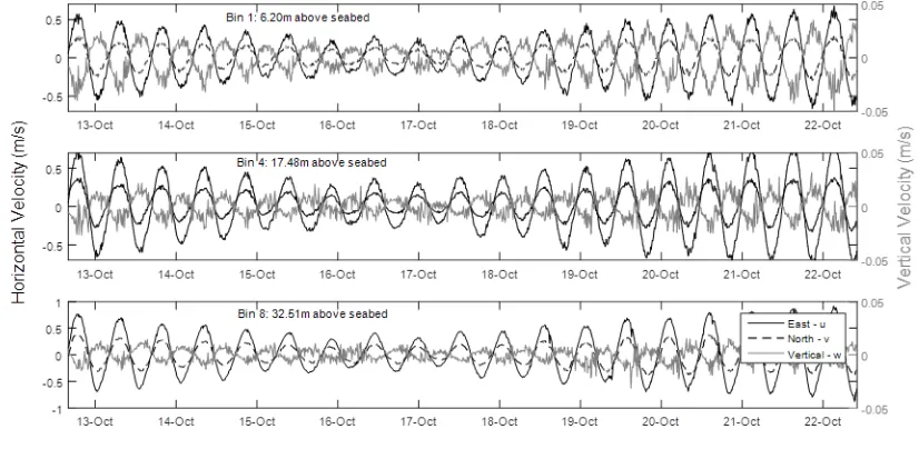
Fig. 6: 10-minute averaged time histories of the u, v and w components during the deployment period.

0 0.2 0.4 0.6 0.8 1 1.2 1.4 1.6 1.8 2

5 10 15 20 25 30 35 40

Velocity (m/s)

H

e

ig

h

t

a

b

o

v

e

s

e

a

b

e

d

(

m

)

Total current velocity Current velocity without Stokes drift

0.2

0.4

0.6

0.8

1

30

210

60

240

90 270

120 300

150 330

[image:19.595.187.406.106.240.2] [image:19.595.207.391.269.441.2] [image:19.595.88.501.494.696.2]

20

Fig. 7: 10-minute averaged time histories of the u, v and w components during four tidal cycles.

Fig. 8: Time series contour plot showing the variation of (total) current speed with height during the deployment.

(a) (b)

Fig. 9: 10 minute time-averaged current velocity profiles over a tidal cycle: (a) near neap tide, (b) near spring tide.

H

e

ig

h

t

A

b

o

ve

S

e

a

F

lo

o

r

-

m

13-Oct-100 14-Oct-10 15-Oct-10 16-Oct-10 18-Oct-10 19-Oct-10 20-Oct-10 22-Oct-10 5

10 15 20 25 30 35

ms

- 1

0.1 0.2 0.3 0.4 0.5 0.6 0.7 0.8 0.9

0 0.2 0.4 0.6 0.8 1 1.2

0 5 10 15 20 25 30 35 40

H

e

ig

h

t

A

b

o

ve

S

e

a

F

lo

o

r

-

m

High Tide Low Tide Flood Ebb

0 0.2 0.4 0.6 0.8 1 1.2

0 5 10 15 20 25 30 35 40

H

e

ig

h

t

A

b

o

ve

S

e

a

F

lo

o

r

-

m

[image:20.595.114.482.106.250.2] [image:20.595.114.499.302.509.2] [image:20.595.112.499.551.673.2]

21

[image:21.595.81.523.73.227.2]

(a) (b)

Fig. 10: (a) Time histories of turbulent intensities at three bin heights during the deployment. (b) Turbulence intensities against mean current speed. Key: at 6.2 m (blue +), 21m (black) and 36 m (red o).

Fig. 11: Reynolds Stresses throughout the deployment. The τvw stresses are in black and the τuw stresses are in grey. The different profiles

indicate the stresses at high tide (+), during the ebb (o), low tide (□) and during the flood (-).

13-Oct-10 14-Oct-10 15-Oct-10 16-Oct-10 17-Oct-10 18-Oct-10 19-Oct-10 20-Oct-10 21-Oct-10 22-Oct-100 10 20 30 40 50 60 70 80 90 100 In te n si ty ( % )

0 0.1 0.2 0.3 0.4 0.5 0.6 0.7 0.8 0.9 1 0 10 20 30 40 50 60 70 80 90 100

Velocity (ms-₁₎

In te n si ty ( % ) -5 0 5

0 5 10 15 20 25 30 35

T id a l C ycl e :H ig h T id e - 1 2 -O ct 2 2 :0 9 to H ig h T id e - 1 3 -O ct 1 0 :2 9 Pa

Height above sea floor - m

-5

0

5

0 5 10 15 20 25 30 35

T id a l C ycl e :H ig h T id e - 1 3 -O ct 2 2 :5 9 to H ig h T id e - 1 4 -O ct 1 1 :1 9 Pa

Height above sea floor - m

-5

0

5

0 5 10 15 20 25 30 35

T id a l C ycl e :H ig h T id e - 1 4 -O ct 2 3 :5 9 to H ig h T id e - 1 5 -O ct 1 2 :2 9 Pa

Height above sea floor - m

-5

0

5

0 5 10 15 20 25 30 35

T id a l C ycl e :H ig h T id e - 1 6 -O ct 0 0 :4 9 to H ig h T id e - 1 6 -O ct 0 7 :3 9 Pa

Height above sea floor - m

-5

0

5

0 5 10 15 20 25 30 35

T id a l C ycl e :H ig h T id e - 1 6 -O ct 1 3 :5 9 to H ig h T id e - 1 7 -O ct 0 3 :1 9 Pa

Height above sea floor - m

-5

0

5

0 5 10 15 20 25 30 35

T id a l C ycl e :H ig h T id e - 1 7 -O ct 1 5 :1 9 to H ig h T id e - 1 8 -O ct 0 3 :5 9 Pa

Height above sea floor - m

-5

0

5

0 5 10 15 20 25 30 35

T id a l C ycl e :H ig h T id e - 1 8 -O ct 1 6 :0 9 to H ig h T id e - 1 9 -O ct 0 4 :2 9 Pa

Height above sea floor - m

-5

0

5

0 5 10 15 20 25 30 35

T id a l C ycl e :H ig h T id e - 1 9 -O ct 1 6 :5 9 to H ig h T id e - 2 0 -O ct 0 5 :1 9 Pa

Height above sea f