An engineering method for modeling the interaction of circular bodies and very low aspect ratio cruciform wings at supersonic speeds

(1)

Tuling, S. (2013) An Engineering Method for Modeling the Interac-tion of Circular Bodies and Very Low Aspect Ratio Cruciform Wings at Supersonic Speeds. PhD, University of the West of England.

We recommend you cite the published version.

The publisher’s URL ishttps://eprints.uwe.ac.uk/secure/21907/

Refereed: No

(no note)

Disclaimer

UWE has obtained warranties from all depositors as to their title in the material deposited and as to their right to deposit such material.

UWE makes no representation or warranties of commercial utility, title, or fit-ness for a particular purpose or any other warranty, express or implied in respect of any material deposited.

UWE makes no representation that the use of the materials will not infringe any patent, copyright, trademark or other property or proprietary rights.

UWE accepts no liability for any infringement of intellectual property rights in any material deposited but will remove such material from public view pend-ing investigation in the event of an allegation of any such infrpend-ingement.

(2)

An Engineering Method for Modeling the Interaction of

Circular Bodies and Very Low Aspect Ratio Cruciform

Wings at Supersonic Speeds

Sean Tuling

A thesis submitted in partial fulfilment of the requirements of the University of the West of England, Bristol

for the degree of Doctor of Philosophy

Faculty of Environment and Technology, University of the West of England, Bristol

(3)

Abstract

An engineering method using a 2D unsteady potential formulation (called the free

vor-tex model or FVM) has been developed to predict the normal force, centre-of-pressure

and vortex position for cruciform wing-body combinations in the “plus” orientation, at

supersonic speeds and cross ﬂow Mach numbers less than or equal to 0.55 up to angles

of attack 20◦. The wings are of very low aspect ratio (≤0.1), have taper ratios greater than 0.85 (or signiﬁcant side edges) and have low span to body diameter ratios (≤1.5). The method predicts the position and subsequent loads imposed by the vortex along the

length on the wing-body combination by determining the shed vorticity using Jorgensen’s

modiﬁed Newtonian impact method. The vortex position is well predicted for angles of

attack from 4◦ until symmetric vortex shedding occurs, whilst the normal force is well predicted from 0◦. The centre-of-pressure is predicted further aft at the low angles and further forward at the high angles of attack. If this method is used in combination with

the single concentrated vortex of Bryson applied to cruciform wing-body combinations the

vortex positions prediction limitations at angles of attack less than 4◦ can be overcome. An investigation of the lee side flow field of cruciform wing-body configurations was also

performed, and revealed that the vortex position is dependent upon the lee side secondary

vortex separation characteristics. Other features revealed that symmetric vortex shedding

occurs when both the region of ﬂow outside the shed vortex sheet and reverse ﬂow region

are supersonic and a termination shock exists. The thesis also investigated the

applica-tion of the discrete vortex model (DVM) method to cruciform wing-body combinaapplica-tions

and found that the potential only formulation overpredicts the normal force, whilst the

inclusion of boundary layer separation (and therefore modeling the secondary separation

vortex) predicted the normal force very well. The application of the concentrated vortex

method of Bryson was also investigated and found to be only applicable at low angles of

(4)

Acknowledgements

I would like to thank my immediate supervisor Laurent Dala for all the questions, guidance,

prompting and sterness required to start and ﬁnish a doctorate. Also my thanks to my

other supervisors Chris Toomer and Mike Ackerman for their guidance.

I would like to thank all the staﬀ at the CSIR who have helped and encouraged,

without which this doctorate would not have progressed at all. In particular to Beeuwen

Gerryts for putting faith in the doctorate and making time available; to Mauro Morelli

and Kaven Naidoo for giving me space and persevering in the process; to Bhavya Vallabh

for the invaluable help; Bronwyn Meyers for all the help on the PIV system, and the test

teams that have helped get the experimental work done.

To all friends and family that have helped and encouraged and given the time and

space.

(5)

Statement of Objectives

The objectives of this research are to add to the knowledge of ﬂows over slender bodies

with very low aspect ratio wings and develop a theoretical or semi-empirical model of

these ﬂows so that they can be used during the preliminary design phases.

All the work in this thesis was performed by the author except for the

following:-• Low speed water tunnel tests that were performed at the University of M´alaga by M.A. Arevalo-Campillos, L. Parras and Dr. Carlos del Pino. A paper summarising

the work performed is listed in Appendix B.

• The High Speed and Low Speed Wind Tunnel tests at the CSIR were performed by teams because of the industrial nature of the facilities. The author did, however,

manage and direct the tests, was a team member setting up and running the tests,

performed quality assurance on, and data reduction for both the tests.

This copy has been supplied on the understanding that it is copyright material and

(6)

List of Figures

1.1 Slender body theory wing body interference factors [4] . . . 22

2.1 Cross ﬂow drag coeﬃcient as a function of Reynolds number for Mach num-bers below 0.4 [42] . . . 36

2.2 Strouhal number variation as a function of Mach number [39] . . . 36

2.3 Types of ﬂows expected for inclined circular bodies and the dependence on angle of attack and Reynolds number. . . 38

2.4 Cross ﬂow drag coeﬃcient as a function of Mach number [42] . . . 39

2.5 Cross ﬂow drag proportionality factor as a function of slenderness ratio [42] 43 2.6 Product of cross ﬂow drag and proportionality factor as a function of Mach number [53] . . . 44

2.7 Cross ﬂow drag proportionality factor as a function of cross ﬂow Mach number [53] . . . 44

2.8 Delta wing ﬂow regimes [72] . . . 47

2.9 Subsonic rectangular wing ﬂow structures [77]. S and N denote saddle and nodal singular points of separation or reattachment as interpreted by reference [77]. . . 48

2.10 Slender body theory wing body interference factors [4] . . . 56

3.1 Cross ﬂow physical and transformed axes systems . . . 64

4.1 Conﬁguration Geometry, dimensions in mm . . . 72

4.2 Body Alone Vortex Start Location . . . 73

4.3 Body and strakes CFD mesh . . . 74

4.4 Strake CFD mesh . . . 75

4.5 Body alone CFD Mach number comparison . . . 76

4.6 Body and strake CFD Mach number comparison . . . 77

4.7 Strakes alone CFD Mach number comparison . . . 78

4.8 Body alone CFD grid sensitivity comparison, Mach 2.0 . . . 79

4.9 Body and strake CFD grid sensitivity comparison, Mach 2.0 . . . 80

4.10 Strakes alone CFD grid sensitivity comparison, Mach 2.0 . . . 81

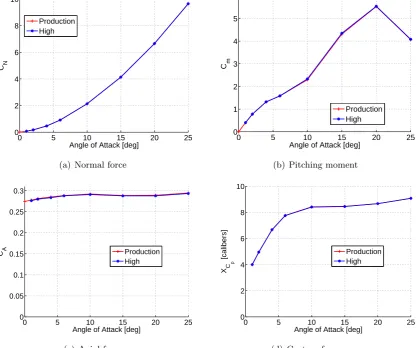
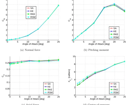
4.11 Body alone CFD turbulence model comparison, Mach 2.0 . . . 83

(11)

4.13 Body alone pressure diﬀerence between SA and RSM turbulence models,

α=2◦ . . . 85

4.14 Body alone CFD and experimental normal and axial force and pitching moment comparison, Mach 2.0 . . . 89

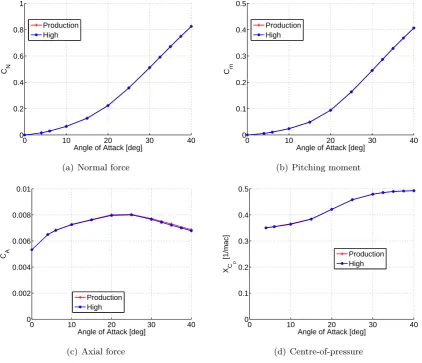
4.17 Body and strakes CFD and experimental normal and axial force and pitch-ing moment comparison, Mach 2.0 . . . 92

4.20 Body alone lateral loads deviation . . . 95

4.21 Body and strakes lateral loads deviation . . . 96

4.22 Schlieren of body alone at M2.0 . . . 98

4.25 Schlieren of body and strake at M2.0 . . . 101

4.28 Water tunnel tests overview . . . 105

4.29 LSWT model in test section . . . 106

4.30 Vortex sheet roll up for LSWT tests for angles lower than 20◦ . . . 107

4.31 Vortex sheet roll up for LSWT tests at angles greater than 17◦ . . . 108

4.32 Body and strake vortex sheet roll up for 20◦ . . . 108

4.33 Vortex trajectories at 11◦ . . . 110

4.37 CFD concentrated vortex positions atα= 2◦ . . . 115

4.38 CFD concentrated vortex positions atα= 4◦ . . . 116

4.39 CFD and experimental comparisons of concentrated vortex positions atα= 6◦117 4.40 CFD and experimental comparisons of concentrated vortex positions at α= 10◦ . . . 118

4.41 CFD and experimental comparisons of concentrated strake vortex positions atα= 15◦ . . . 119

(12)

4.43 CFD and experimental comparisons of concentrated body vortex positions

atα= 20◦ . . . 121

4.44 CFD and experimental comparisons of concentrated body vortex positions atα= 20◦ . . . 122

4.45 CFD and experimental comparisons of concentrated strake vortex positions atα= 25◦ . . . 123

4.46 CFD and experimental comparisons of concentrated body vortex positions atα= 25◦ . . . 124

4.47 Body vortex comparison for angles of attack of 6◦, 10◦ and 15◦ at 4.75D . . 125

4.48 Body vortex and cross ﬂow Mach number comparison for angles of attack of 10◦ and 15◦ at 4.75D . . . 126

4.49 Side edge vortex development as a function of angle of attack . . . 128

4.50 Vortex development for strake only forα= 10◦ at Mach 2.0 . . . 129

4.55 Vortex development for strake only at Mach 2.5 and 3,0 . . . 132

4.56 Strake eﬀect on full conﬁguration normal force as a function of angle of attack133 4.57 Body and strake side edge vortex atα= 4◦ . . . 134

4.58 Body and strake side edge vortex atα= 10◦ . . . 134

4.61 Vortex development forα= 1◦, body compared to body and strake at Mach 2.0 . . . 136

4.65 Vortex development for α = 10◦, body compared to body and strake at Mach 2.0 . . . 138

(13)

4.70 Installed strake normal force comparison . . . 142

4.71 Wing-to-Body carryover factor . . . 143

4.72 Aftbody vortex shedding at 25◦ at Mach 2.0 . . . 144

4.73 Body alone cross ﬂow Mach number and vortex position at Mach 3.0 at α= 10◦ . . . 146

4.76 Strake cross flow Mach number and vortex position at Mach 2.0 atα= 20◦ 149 4.77 Strake cross flow Mach number and vortex position at Mach 2.0 atα= 25◦ 150 4.78 Strake cross flow Mach number and vortex position at Mach 2.0 atα= 30◦ 151 4.79 Body and strakes cross flow Mach number and vortex position at Mach 3.0 atα= 10◦ . . . 152

4.80 Body and strakes cross ﬂow Mach number and vortex position at Mach 3.0 atα= 15◦ . . . 153

4.81 Body and strakes cross ﬂow Mach number and vortex position at Mach 3.0 atα= 20◦ . . . 154

4.82 Lee side body strake junction secondary vortex at Mach 2.0 atα = 2◦ . . . 156

5.1 Vortex path for angle of attack 10◦ (in the circle plane) . . . 167

5.2 CFD and SCV normal force and centre-of-pressure comparison . . . 169

5.3 Vortex development forα = 1◦, SCV . . . 170

5.11 CFD and SCV concentrated vortex position comparison atα= 2◦ . . . 179

5.14 CFD and SCV comparisons of the non-dimensionalised concentrated vortex strength for 2◦ and 4◦ . . . 183

(14)

6.1 Vortex path as a function of step size (in the circle plane) . . . 195

6.2 Vortex strength as a function of step size . . . 195

6.3 Kutta edge velocity as a function of step size . . . 196

6.4 CFD and DVM normal force and centre-of-pressure comparison . . . 198

6.5 Vortex development forα = 1◦, potential only . . . 199

6.13 Vortex development forα = 1◦, potential+boundary layer . . . 207

6.21 Vortex development forα = 1◦, potential+boundary layer at 5% . . . 215

6.29 CFD and DVM concentrated vortex positions atα= 2◦ . . . 224

6.30 CFD and DVM concentrated vortex positions atα= 4◦ . . . 225

6.31 CFD and DVM comparisons of concentrated vortex positions atα= 6◦ . . 226

6.32 CFD and DVM comparisons of concentrated vortex positions atα= 10◦ . . 227

6.33 CFD and DVM comparisons of concentrated strake vortex positions atα= 15◦ . . . 228

6.34 CFD and DVM comparisons of concentrated body vortex positions atα= 15◦229 6.35 CFD and DVM comparisons of concentrated strake vortex positions atα= 20◦ . . . 230

(15)

6.38 CFD and DVM comparisons of concentrated body vortex positions atα= 25◦233 6.39 CFD and DVM comparisons of the non-dimensionalised concentrated vortex

strength for α= 2◦ and 4◦ . . . 234

6.40 CFD and DVM comparisons of the non-dimensionalised concentrated vortex strength for α= 6◦ and 10◦ . . . 235

6.41 CFD and DVM comparisons of the non-dimensionalised concentrated vortex strength for α= 15◦ and 20◦ . . . 236

7.1 CFD and FVM normal force and centre-of-pressure comparison . . . 243

7.2 Normal force coeﬃcient increment at 4◦ and 10◦ along the body length . . . 245

7.3 Vortex development forα = 1◦, FVM . . . 246

7.11 CFD and FVM concentrated vortex positions atα= 2◦ . . . 254

7.12 CFD and FVM concentrated vortex positions atα= 4◦ . . . 255

7.13 CFD and FVM comparisons of concentrated vortex positions atα= 6◦ . . 256

7.14 CFD and FVM comparisons of concentrated vortex positions atα= 10◦ . . 257

7.15 CFD and FVM comparisons of concentrated strake vortex positions atα= 15◦258 7.16 CFD and FVM comparisons of concentrated body vortex positions atα= 15◦259 7.17 CFD and FVM comparisons of concentrated strake vortex positions atα= 20◦260 7.18 CFD and FVM comparisons of concentrated body vortex positions atα= 20◦261 7.19 CFD and FVM comparisons of concentrated strake vortex positions atα= 25◦262 7.20 CFD and FVM comparisons of concentrated strake vortex positions atα= 25◦263 7.21 CFD and FVM comparisons of the non-dimensionalised concentrated vortex strength for α= 2◦ and 4◦ . . . 265

7.22 CFD and FVM comparisons of the non-dimensionalised concentrated vortex strength for α= 6◦ and 10◦ . . . 266

7.23 CFD and FVM comparisons of the non-dimensionalised concentrated vortex strength for α= 15◦ and 20◦ . . . 267

7.24 CFD and FVM normal force and centre-of-pressure comparison for Mach 1.5270 7.25 CFD and FVM concentrated vortex positions atα= 4◦ for Mach 1.5 . . . . 272

7.26 CFD and FVM concentrated vortex positions atα= 6◦ for Mach 1.5 . . . . 273

7.27 CFD and FVM concentrated vortex positions atα= 10◦ for Mach 1.5 . . . 274

7.28 CFD and FVM concentrated vortex positions atα= 15◦ for Mach 1.5 . . . 275

(16)

7.30 NASA TM-X-3130 model conﬁguration . . . 277

7.31 CFD and FVM normal force and centre-of-pressure comparison for the NASA TM-X-3130 N1C1S conﬁguration . . . 278

7.32 NASA TM-X-1839 model conﬁguration, dimensions in inches . . . 279

7.33 CFD and FVM normal force and centre-of-pressure comparison for the NASA TM-X-1839 N1C1S conﬁguration . . . 280

7.34 Simpson and Birch B11AW22A3 model conﬁguration . . . 281

7.35 CFD and FVM normal force and centre-of-pressure comparison for the W22 conﬁguration . . . 282

7.36 NASA TM-2005-213541 Triservice model conﬁguration, dimensions in inches 283 7.37 CFD and FVM normal force and centre-of-pressure comparison for the NASA TM-2005-213541 Triservice conﬁguration . . . 284

A.1 Vertical vortex position predictions,α= 10◦ . . . 303

A.2 Lateral vortex position predictions,α= 10◦ . . . 303

A.3 Vertical vortex position predictions,α= 20◦ . . . 304

(17)

List of Tables

2.1 Computational accuracy requirements [22] . . . 25

2.2 Coeﬃcient accuracy requirements [22] . . . 25

2.3 Missile Datcom body alone computational methods . . . 27

2.4 Missile Datcom wing and interference computational methods . . . 27

2.5 NSWC body alone computational methods [22] . . . 28

2.6 NSWC wing and interference computational methods [22] . . . 29

2.7 AERODYN body alone computational methods [22] . . . 30

2.8 AERODYN ﬁn and interference computational methods [22] . . . 31

3.1 Cross ﬂow drag coeﬃcient . . . 70

4.1 Experimental test conditions . . . 87

4.2 Experimental test accuracies . . . 87

6.1 Estimated CFD Body Vortex Positions and Strengths . . . 194

(18)

List of Symbols

APC Aeroprediction Code

AR Aspect ratio,b2/S

a Radius

b Span

cdc Cross ﬂow drag coeﬃcient

CA Axial force coeﬃcient, body axes

CD Drag coeﬃcient

CFL Courant-Friedrich-Lewy

CL Lft coeﬃcient (wind axes)

Cl Rolling moment coeﬃcient (body axes)

Cm Pitching moment coeﬃcient (body axes)

Cn Yawing moment coeﬃcient (body axes)

CN Normal force coeﬃcient (body axes)

CmBW T Pitching moment coeﬃcient for body, wing and tail conﬁguration

CNBW T Normal force coeﬃcient for body, wing and tail conﬁguration

CNB Normal force coeﬃcient for isolated body

CNB(T) Normal force coeﬃcient increment of body due to the tail

CNT(B) Normal force coeﬃcient increment of tail due to the body

CNB(W) Normal force coeﬃcient increment of body due to wing

CNW(B) Normal force coeﬃcient increment of wing due to body

CNT(W) Normal force coeﬃcient increment of tail due to wing

CNα Normal force coeﬃcient slope (with respect to α)

Cp Pressure coeﬃcient

Cpρ Non-dimensionalised loss in maximum mainstream dynamic head

CPU Central Processing Unit

CSIR Council for Scientiﬁc and Industrial Research

CY Side force coeﬃcient, body axes

D Body diameter

DVM Discrete Vortex Model

FA Axial force, body axes

(19)

FN Normal force, body axes

FNv Normal force due to vortex, body axes

FVM Free Vortex Model

FY Side force, body axes

HSWT High Speed Wind Tunnel

iT Tail interference factor due to a free vortex

KBW Wing-to-body carryover factor

kB Fin deﬂection interference factor, wing-to-body

KE κ−ϵturbulence model

KWB Body-on-wing carryover factor

kW Fin deﬂection interference factor, body on wing

Kϕ Additional loading due to roll angle at constant angle of attack

L Body length, lift

LSWT Low Speed Wind Tunnel

M Freestream Mach number

Mc Cross ﬂow Mach number,M sin(α)

MN Mach number normal to the leading edge

n Vortex shedding rate

q Freestream dynamic pressure, 1/2ρV_∞2

Re Reynolds number

RKE Realisableκ−ϵturbulence model RSM Reynolds-Stress model

ro Radius of the circle in the circle plane

rB Radius at the base

S Reference area, usuallyπD2_/4

SB Body base area

Sp Planform area

SA Sparlat-Allmaras

s Span of exposed ﬁn/wing

sm Wing-body semi-span

SBT Slender Body Theory

SCV Single Concentrated Vortex

SOSE Second Order Shock Expansion

SSB Stanbrook and Squire Boundary

u Velocity pertubation in the x-axis direction

ue Surface velocity

V Freestream velocity

Vc Cross ﬂow velocityV sin(α)

(20)

xs Axial location of start of body vortices, from nose

yv Body vortex location in lateral direction

zv Body vortex location in vertical direction

α Angle of attack

αN Angle of attack normal to the leading edge

δ Fin deﬂection angle

δs Boundary layer vorticity reduction factor

∆αv Induced angle of attack due to a vortex

η End eﬀect factor

ηn Half angle of sharp nose

Γ Vortex strength

Γ′ Non-dimensionalised vortex strength, ₂_{πV a}Γ

γ Speciﬁc heat ratio

γl Line vortex strength

Λ Fin on ﬁn inﬂuence factor

Φ Inertial axes velocity potential

ϕ Body axes velocity potential

ϕx Roll angle

ρ Air density

(21)

Chapter 1

Introduction

The prediction of aerodynamic loads of airframes has been the subject of aerodynamicists

for over a century. For aircraft type conﬁgurations, the Joukowski-Kutta condition and

lifting line theory were signiﬁcant developments in the ability to model and predict

aerody-namic loads for wings. For bodies, the primary theory was originally developed by Munk

[1] and extended by numerous researchers. Missiles are characterised by slender bodies

and low aspect ratio lifting surfaces. For missiles, body wing interactions contribute

sig-niﬁcantly to the overall aerodynamic loads of the conﬁguration compared to aircraft type

conﬁgurations. These interactions have, in part, contributed to the creation of the class

of ﬂuid ﬂow known as missile aerodynamics.

The primary methods for predicting missile aerodynamics at an engineering level were

developed in the late 1950’s and early 1960’s by numerous investigators such as Morikawa

[2], Allen and Perkins [3] and summarised in the ﬁrst textbook dedicated to missile

aero-dynamics by Nielsen [4]. These methods relied on potential slender body theory, which

is strictly applicable to only low angles of attack (≤4◦), and through insightful ’assump-tions’ and heuristic analogies extended to moderate (≈ 10◦) and higher angles of attack (15◦ < α < 25◦). These theories have formed the backbone of the predictive methods for slender body conﬁgurations. Some major developments have occurred in subsequent

decades extending the methods to high angles of attack (α≥25◦). Surprisingly, the use of low angle attached ﬂow slender body theory has been successfully extended to the higher

angles where separated flow are required by slender configurations to generate sufficient

lift forces. Domains where these extensions break down exist, and together with the body

wing interactions are the subject of this thesis.

Before continuing, it should be noted that this thesis is concerned with the interaction

of circular bodies of constant diameter and wings whose aspect ratio is less than or equal

to 0.1 or alternatively described as very low aspect ratio wings. The very low aspect ratio

wings are also commonly called strakes, and both very low aspect ratio wings and strakes

shall be used interchangeably throughout the thesis. Furthermore the strakes have limited

(22)

to body diameter ratio is 1.25. These and other limitations placed on this research are as

follows:-• Strake aspect ratios of the order 0.025 (and less than 0.1)

• Strake taper ratios greater than 0.85

• Strake span to body diameter ratios of 1.25

• Supersonic Mach numbers

• Cruciform wings in the ’+’ conﬁguration

• Wing-body section of constant body diameter

• Wing length is a signiﬁcant proportion (>50%) of the overall body length

The angle of attack regime being considered in this thesis is from zero to 25◦, and low angles are considered α ≤ 4◦, moderate angles from 4◦ to 15◦ and the higher angle of attack regime from 15◦ to 25◦. High angles of attack are traditionally considered as greater than 25◦ and is the case in this thesis too.

1.1

Thesis

The research question being answered is how can very low aspect ratio wing-body

inter-actions be modeled at an engineering level, and in particular the wing-to-body carryover

factor, for engineering prediction purposes. The thesis put forward is that the side edge

vortex shed by very low aspect ratio wings with signiﬁcant side edges, being non-linear

in nature, interacts signiﬁcantly with the body such that the aerodynamics of such

con-ﬁgurations needs to be modeled together. This results in the non-linear behaviour of the

wing-to-body carryover factor, KBW, with angle of attack. In particular, the side edge

shed vortex is the dominant ﬂow phenomenon whose motion when treated as a Lagrangian

ﬂuid particle can predict the motion of the side edge vortex suﬃcient well for engineering

prediction purposes. Finally an integrated method is proposed which forms the basis for

the better modeling ofKBW, and therefore extending the previous formulations and which,

in ﬁrst order, account for the non-linear eﬀects.

1.2

Background

The total normal (or lift) force on a slender body-wing conﬁguration has, for one school

of thought, been traditionally based on the build up method of conﬁgurations (i.e. the

addition of wings and/or tails to a slender body) by the linear summation of the individual

components (i.e. body alone and wing alone) and their interference factors (i.e.

(23)

CNBW T =CNB+CNW(B) +CNB(W)+CNT(B) +CNB(T) +CNT(W) (1.1)

whereCNB is the isolated body,CNW(B), the wing in the presence of the body,CNB(W),

the increment of the body due to the wing, CNT(B), the tail in the presence of the body,

CNB(T), the increment of the body due to the tail, andCNT(W) the eﬀect of the wing on

the tail. For a conﬁguration that does not have a tail, which the subject of this thesis is

restricted to, the last three terms are excluded.

The wing in the presence of the body, CNW(B), is can be written in terms of the wing

alone CNW, which is made up by combining the two exposed halves of the wing, as has

been traditionally deﬁned. The planform characteristics of the wings under consideration

are deﬁned in terms of the wing alone. CNW(B) has been traditionally deﬁned in terms of

the body-on-wing carryover factor,KWB, [4] or

CNW(B) =KWBCNW (1.2)

The body-on-wing carryover factor includes the contribution of the wing alone and the

incremental or interference eﬀect due to the body. For the interference eﬀect of the wing

onto the body, or wing-to-body carryover, this has also been deﬁned in terms of the wing

alone characteristics [4], and is deﬁned as

CNB(W) =KBWCNW (1.3)

Equation 1.1 can, for this thesis, be written as

CNBW =CNB + (KWB +KBW)CNW (1.4)

The original theories developed to predict the aerodynamics of slender body-wing

conﬁgurations are based on linear analysis [4]. They assume that the body and the wings

have linear characteristics with angle of attack. For bodies at angles of attack larger than

4◦ non-linear effects start to become significant, primarily due to the shedding of vortices (up to 4◦the flow remains attached even though the lee side boundary thickens as the angle of attack increases from 0◦). For engineering level predictions, a heuristic model based on the cross-flow concept was proposed by Allen [5] and has been used with considerable

success since its introduction such that it remains the starting point for any engineering

prediction code such as Missile Datcom and Aeroprediction code (APC). For wings of

aspect ratio of the order 1, the normal force can be considered linear up to angles of

attack of approximately 40◦[4] whereupon non-linear eﬀects (stall and vortex breakdown) dominate. This is because the leading and side edge vortices are not a large contribution

to the overall lift force. The theoretical lift curve slope of a low aspect ratio wing with

(24)

interaction factors because the wing alone lift characteristics can be formulated based on

the linear lift curve slope, or

CNW =

( ∂CNW

∂α )

α=0◦

α (1.5)

Traditionally the values used to model the the wing-to-body,KWB, and body-on-wing,

KBW, factors are derived from slender body theory. The eﬀect of afterbodies on these

carryover factors have also been considered and are based on two fundamental assumptions,

namely that the ﬂow over the wing is conical and that the body is modelled as a plane

rather than a circular body [4][7]. This formulation assumed that the aft body is of

suﬃcient length to ’catch’ the wing eﬀect. Formulations accounting for zero-,

limited-and negative aft bodies were developed in references [8],[9] limited-and [10]. The body-on-wing

carryover factor, KWB, or the “Beskin” upwash factor is due to the induced velocity of

the body increasing the eﬀective incidence of the wing, whilst the wing-to-body carryover

factor,KBW, has been essentially interpreted as the body increasingly acting as a reﬂection

plane for the wing as the wing semi-span reduces. The development of the equivalent angle

of attack method [11] in the early 1980’s accounts for non-linearities in the lift curve slope

of wings and extends the low angle of attack method of the previous equations to high

angles of attack, and made the component buildup method applicable up to 60◦.

A limitation in the previously developed methodologies observed in recent decades has

been for the combination of very low aspect ratio wings and slender bodies [12][13], this

being the modelling of the wing-to-body interference factor,KBW. This limitation includes

the equivalent angle of attack method. When very low aspect ratio wings (AR=0.067

in reference [13]) are combined with slender bodies having a chord of similar length to

the slender body length, the wing-to-body carry over factor, KBW, is underpredicted by

approximately 50% at low and moderate angles of attack. The traditional formulation

of KBW is based on slender body theory; and in the limit of a wing of zero span, the

carryover factor is 2.0. These are graphically displayed in Figure 1.1.

One other factor that has been demonstrated to inﬂuence KBW is the cross ﬂow Mach

number,Mc=Msinα[14]. The eﬀect of the cross ﬂow Mach number is that the carryover

factors dissipate to 1 forKWB and 0 forKBWwhen the cross ﬂow Mach number is greater

than 0.3. The data presented by Simpson and Birch shows neither these eﬀects for KWB

and KBW for their tests performed at Mach 2.5 (resulting in a cross ﬂow Mach number

of 1.05 at an angle of attack of 25◦). Indeed KWB does not drop by more than 20%

over the angle of attack range of 25◦ whilstKBW, even though underpredicted, does not

drop to zero at 25◦. The data presented by reference [14] were for wings of aspect ratio AR=0.5. From the available literature the eﬀect very low aspect ratio wings on slender

body conﬁgurations is not well modeled and the purpose of this body of work is to propose

an extended formulation for KBW that will improve the prediction of the eﬀect of very

(25)

0 0.2 0.4 0.6 0.8 1 0

0.2 0.4 0.6 0.8 1 1.2 1.4 1.6 1.8 2

a/s

m

K

W

B

K

B

[image:25.595.182.493.55.319.2]

W

Figure 1.1: Slender body theory wing body interference factors [4]

Wings of very low aspect ratio i.e. less than 0.1, are not uncommon, though fewer

practical conﬁgurations tend to exist because wings of higher aspect ratio provide a more

eﬃcient way of generating lift. The beneﬁts of very low aspect ratio wings for slender

bodies have been recognised [15] where lower drag and space constrained conﬁgurations

are required. At least up until the early 1980’s no attempts had been made to develop

engineering level methods of predicting the eﬀect of very low aspect ratio wings in slender

body conﬁgurations. From the late 1980’s onwards, attempts to better model the eﬀect of

wings on bodies have been based on experimental data, such as those for the Aeroprediction

code [16] and Missile Datcom [17][18][19]. APC ﬁts curves to the experimentalKBW data

as a function of Mach number and angle of attack, while Missile Datcom (post 1999)

modifies the cross flow drag coefficient utilising empirical data.

In the past the eﬀect of the wing/strake side edge vortex development in the presence

of the body has been noted but not explicitly accounted for. Once free of the lifting

surface, the eﬀect of the vortex on downstream surfaces will aﬀect both the store pitching

moment and lift characteristics. Two methods have been used in the past. The ﬁrst, as

implemented by Missile Datcom, is to assume that the vortex which is shed from the low

aspect ratio wing emanates from the trailing edge at a lateral distance dependent on the

spanwise lift distribution [7]. The second is to assume that the side edge vortex leaves the

leading edge edge at one half the angle of attack of the wing [20] as deﬁned by Bollay [21].

These two represent two extremes in which the side edge vortex of a strake lies somewhere

(26)

almost rectangular wings) and not highly swept back leading edges have hitherto not been

modeled in the past.

In this thesis it is proposed that this non-linear eﬀect is primarily due to the vortex

separation of the side edge that is not accounted for in the original linear formulations

or the equivalent angle of attack method. For slender body conﬁgurations with very low

aspect ratio wings/strakes the side edge vortex created by the wing interacts with, or is

inﬂuenced by the body, to the extent that the wing and body must be considered together

rather than as separate components whose interactions can be accounted for in a linear

fashion. Consequently the eﬀect of the side edge vortex on downstream bodies and lifting

surfaces will depend on the position and strength of this side edge vortex.

The subject of this thesis is derived directly from industrial applications where the use

of very low aspect ratio wings or strakes have and are being considered for short range

air-to-air missiles for reasons which include space limitations in stealth platforms. The typical

slenderness ratio of such missiles varies from between 17 to 22, while the operational Mach

range is 0.6 to 3.0. This thesis is studying the aerodynamics in the supersonic ﬂight regime

and the range 2.0 to 3.0 has therefore been chosen whilst the low supersonic limit of 1.5

has been excluded because of limitations in experimental validation capabilities.

1.3

Thesis Outline

The subsequent chapters of the thesis ﬁrstly survey the available literature. The core

method is then presented after which the aerodynamics of conﬁguration used to develop the

method is explored. The 2D potential methods with their extensions that are used to study

the conﬁguration are then presented with their predictions after which the engineering

method is assessed further by comparing predictions to the limited publically available

cases. Finally conclusions are drawn, recommendation made and the contributions to the

(27)

Chapter 2

Literature Survey

The survey will start with a general overview of the background theories and methods

used in the preliminary design phase, the potential equation, basic available theories and

their applicability. With a view to surveying the interaction of slender bodies and wings,

work performed on isolated bodies, isolated wings, and combinations of both, and these

within the broader context of engineering methods shall be considered. At this stage it

must be mentioned that the cornerstone of most of the available theories for predicting

the aerodynamics of slender body conﬁgurations is slender body theory (SBT). Slender

body theory is applicable over the complete Mach range thus making it suitable for use

in engineering methods [4].

2.1

The Use of Analytical and Semi-Empirical Methods in

Preliminary Design

The focus of the prediction methods used are analytical and semi-empirical methods.

Analytical methodologies are limited in their capabilities because the full Navier-Stokes

and even the full potential formulation is not mathematrically tractable. They do, however,

provide the basis with which usable semi-empirical methodologies can be developed. The

cornerstone of missile preliminary design prediction methodologies is the slender body

theory (SBT) [14], whose basis is the potential theory applied to slender bodies.

2.1.1 Design Accuracies

In order to contextualise engineering level prediction methodologies it would be useful

to determine their requirements by the users (primarily designers and aerodynamicists)

of such methodologies. During preliminary design, the prevailing accuracies required for

(28)

Table 2.1: Computational accuracy requirements [22]

Design Parameter Value Unit

Range 10 %

Turn radius 20 %

Turn rate 20 %

Load factor 20 %

Speciﬁc Excess Power 100 fps

Fin panel area 20 %

Manoeuver deceleration 20 %

Cruise altitude 1000 ft

Response time 20 %

Center of gravity 2 %body length

[image:28.595.174.506.154.374.2]

Static stability/cross coupling parameters 25 %

Table 2.2: Coeﬃcient accuracy requirements [22]

Coeﬃcient Value Unit Design Parameter

CL 20 % Range, load factor

Cm 20 % Fin size or

or 2 %length Static margin

CA 10 % Coast range or

(29)

2.1.2 Existing Codes and their Prediction Methodologies

The engineering level codes that have been developed in the past utilise a combination of

theoretical and/or experimental data. Numerous codes have been developed in the past,

with varying degrees of accuracy in their predictions [22].

The codes predominantly use the slender body theory as a base foundation with unique

implementations for the nonlinear regions. Their accuracies in the linear low angle of

attack regions are good (within the 20% requirement) and it is in the non-linear (viscous

normal force and pitching moment) and interference areas where diﬀerences appear as

to how these are accounted [22]. For the body alone, they predominantly use the Allen

and Perkins (or derivative forms such as that by Jorgensen) viscous cross-ﬂow method

to account for viscous eﬀects. The loads for the wings and tails have been determined

using a variety of methods (eg. slender body, modiﬁed Multhopp). For the complete

conﬁguration, the buildup methodology is widely used and algebraically sums the various

components and their interference eﬀects [14]. The development of the equivalent angle

of attack method has extended this formulation into the non-linear region [11]. A variety

of methods are also available for the eﬀect of upstream vortices on wings and ﬁns.

A list of codes that have been developed are

• Missile Datcom

• ESDU

• NSWC I & II (Naval Surface Weapon Center) and Aeroprediction (APC)

• MISSILE I, II & III

• AERODYN

• MAP (Missile Aerodynamics Prediction)

• AEDC High Alpha Code

• Army/Martin High Angle-of-Attack Methodology

• DLCODE

• S/HABP (Supersonic/Hypersonic Arbitrary Body Program)

• NSRDC

• NASA W-B-T

• David Taylor (NSRDC I)

• CAMS (Computer Aided Missile Synthesis)

(30)

Most of these codes are not publicly available. Some may not even be used. These have

been predominantly obtained from reference [22] and the subsequent sections detailing

their methodologies are also obtained from the same reference.

2.1.3 USAF Missile Datcom

Missile Datcom uses a large number of diﬀerent theoretical and empirical techniques which

are applied to the components that make up the body alone aerodynamics, wing alone

aerodynamics and interference factors [23][24].

Table 2.3: Missile Datcom body alone computational methods Component Mach

Number

Subsonic Transonic Low

Super-sonic

High

Super-sonic

Axial Force (α= 0) Empirical Empirical & Second Order Van Dyke or

Second Order Shock

Axial Force (α >0) Modiﬁed cross-ﬂow (Jorgensen)

Inviscid Lift and

Pitch Moment

Empirical Van Dyke Hybrid or Second Order Shock

Expansion or Modiﬁed Newtonian

Viscous Lift and

Pitching Moment

Modiﬁed cross-ﬂow (Jorgensen)

Table 2.4: Missile Datcom wing and interference computational methods Component Mach

Number

Super-sonic

High

Super-sonic

Linear Lift

Lowry-Polhamus

Linear Theory

Linear Pitching

Mo-ment

Empirical

Non-linear Lift and

Pitching Moment

Empirical & Panel Centroid

Wing Body

Interfer-ence

Slender Body Theory, Empirical & Equivalent AoA

Wing Tail

Interfer-ence

Slender Body Theory & Line Vortex Theory

2.1.4 ESDU

ESDU uses the Pitts, Nielsen and Kaattari slender body theory for the potential ﬂow

(31)

component is modiﬁed with experimental data for the subsonic, transonic and supersonic

regimes taking accounting for factors such as end length.

2.1.5 NSWC & APC

The NSWC code utilises basic theoretical methods for many of its components. It also

makes signiﬁcant use of CFD correlated with experimental data. The Aeroprediction code

(APC) is the latest code development [16].

Table 2.5: NSWC body alone computational methods [22]

Component Mach

Number

Super-sonic

High

Super-sonic

Nose Wave Drag - Euler plus

Empirical

Second Order

Van Dyke

Modiﬁed

Newtonian

Second

Or-der Shock

Expansion

Plus

Modi-ﬁed

Newto-nian

Boattail Wave Drag - Wu &

Aoy-oma

Second Order

Van Dyke

Second

Or-der Shock

Expansion

Skin Friction Drag Van Driest II

Base Drag Empirical

Inviscid Lift and

Pitch Moment

Empirical Euler or Wu

& Aoyoma

plus

Empiri-cal

Tsien First

Order

cross-ﬂow

Second

Or-der Shock

Expansion

Viscous Lift and

Pitching Moment

(32)

Table 2.6: NSWC wing and interference computational methods [22] Component Mach

Number

Super-sonic

High

Super-sonic

Inviscid Lift and

Pitch Moment

Lifting

Sur-face Theory

Empirical Linear

The-ory

Shock

Ex-pansion

The-ory

Wing Body

Interfer-ence

Slender Body Theory and

Empirical

Linear

The-ory, Slender

Body Theory

and

Empiri-cal

-Wing Tail

Interfer-ence

Line Vortex Theory

Wave Drag - Empirical Linear

The-ory +

Mod-iﬁed

Newto-nian

Shock

Ex-pansion +

Modiﬁed

Newtonian

Strip Theory

Skin Friction Drag Van Driest

Trailing Edge

Sepa-ration Drag

Empirical

Body Base Pressure

Drag Caused by Tail

Fins

(33)

2.1.6 MISSILE I, II & III

Missile I, II, III and subsequent developments (M3FLR, M3HAX, M3F3CA) are based

on the body buildup methodology. The body alone method uses slender body theory

plus cross-ﬂow [28],[29]. The wing and tail ﬁn loads are determined from experimental

databases. The equivalent angle of attack method is primarily used to account for

inter-ference eﬀects. The codes are heavily dependent on databases and are thus more empirical

than the code of NSWC for instance.

2.1.7 AERODYN

The AERODYN code utilises basic theoretical methods with empirical corrections, as

summarised in Table 2.7 and 2.8.

Table 2.7: AERODYN body alone computational methods [22]

Component Mach

Number

Super-sonic

High

Super-sonic

Tangent Ogive - Empirical Table

Nose Wave Drag Cone - Semi-Empirical Correlation

Von Karman - Empirical Correlation

Boattail Wave Drag Empirical Table

Skin Friction Drag Van Driest II

Base Drag Empirical (NASA)

Lift (Viscid and

In-viscid)

Modiﬁed Jorgensen

Pitching Moment

(Viscid and

Invis-cid)

(34)

Table 2.8: AERODYN ﬁn and interference computational methods [22]

Component Mach

Number

Super-sonic

High

Super-sonic

Inviscid Lift Lifting-Line Theory and Datcom Theoretical

Viscous Lift Datcom Empirical

Subsonic - Linearised Pertubation Theory

Pitching Moment Transonic Fairing

Supersonic - Lifting Surface Theory

Wing Body

Interfer-ence

Slender Body Theory

(NACA 1307)

Linear Theory, Slender

Body Theory and

Empiri-cal (NACA 1307)

Wing Tail

Interfer-ence

Line Vortex Theory (NACA 1307)

Wave Drag Linear Theory & Empirical

Skin Friction Drag Van Driest III

Vortex

Track-ing/Shadowing

Line Vortex Theory (NACA 1307)

2.1.8 MISSILE (ONERA)

The French Aeronautics Research Organisation, ONERA, utilises the basic Allen and

Perkins formulation (inviscid and viscous) extended by Jorgensen and modify with

ex-perimental data [30]. The interference factors are calculated using the equivalent angle

of attack method and experimental correlations which include parameters such as Mach

number, taper ratio, angle of attack.

2.1.9 NASA W-B-T

The NASA W-B-T code is the method of Jorgensen of reference [31] and utilises a

combina-tion of theoretical methods (Allen and Perkins method extended by Jorgensen), empirical

data and the modiﬁed Newtonian impact theory. The wings are not modeled separately

and the equivalent angle of attack method is not used. Also no vortex tracking to account

for the effect of one fin set on a downstream fin set is implemented.

2.2

Basic Aerodynamic Theories

Missile aerodynamics, at least for engineering predictions, uses a wide range of theories.

The main equation on which almost all of the engineering level missile aerodynamics is

based upon is the potential equation, which describes the velocity potential, Φ, of the ﬂow

(35)

2.2.1 Nonlinear Potential Equation

The form of the equation is determined by number of conditions namely:

• Compressibility of the ﬂuid

• Coordinate system used

• Velocity of the coordinate system with respect to the far ﬁeld fuild

For the case where the ﬂuid is stationary and a missile is moving through the ﬂuid

ﬁeld, the full nonlinear equation for the velocity potential, Φ, is

[

c2_∞−(γ−1) (

Φτ +

Φ2_ξ+ Φ2_η+ Φ2_ζ 2

)]

(Φξξ+ Φηη+ Φζζ)

= Φτ τ+ (Φ2ξ+ Φξξ+ Φ2ηΦηη+ Φζ2Φζζ) + 2(ΦξΦηΦξη+ ΦξΦζΦξζ

+ΦηζΦηΦζ) + 2(ΦξΦξτ + ΦηΦητ + ΦζΦζτ) (2.1)

The axes system that is fixed to the fluid is ξ, η, ζ. c represents the speed of sound of the fluid in the far field, while τ, is time.

In many cases, the situation that is of interest, is where the missile is stationary with

respect to the observer, and the ﬂuid is assumed to be moving at velocity and is parallel

and uniform. The axes ﬁxed to the missile, x, y, z, at time t, is such that x is parallel to the ﬂuid traveling at velocity, V. Transforming the potential equation 2.1 using the following equations:

¯

x = ξ+V τ ¯

y = η

¯

z = ζ

t = τ (2.2)

results in the new velocity potential,ϕ

[

c2+γ−1

2 V −(γ−1) (

ϕt+

ϕ2_x_¯+ϕ2_y_¯+ϕ2_z_¯ 2

)]

(ϕx¯¯x+ϕy¯y¯+ϕz¯¯z)

=ϕtt+ (ϕ2x¯+ϕx¯x¯+ϕ2y¯ϕy¯y¯+ϕ2z¯ϕz¯z¯) + 2(ϕx¯ϕy¯ϕx¯y¯+ϕx¯ϕz¯ϕx¯z¯

+ϕy¯z¯ϕy¯ϕz¯) + 2(ϕx¯ϕxt¯ +ϕy¯ϕyt¯ +ϕz¯ϕzt¯) (2.3)

2.2.2 Linearised Potential Equation

The linearised potential equation is derived from the nonlinearised equation by assuming

(36)

or at least an order of magnitude smaller than the free-stream velocity. The linearised

equation can be written as

c2∇ϕ2 =ϕtt+V∞ϕ¯xx¯+ 2ϕ¯xt (2.4)

Expressing this in terms of the Mach number M, which equals

M = V

c (2.5)

The linear potential equation can be written as

ϕx¯x¯(1−M2) +ϕy¯y¯+ϕ¯zz¯= 1 c2

∞

ϕtt+ 2

M

c ϕxt¯ (2.6)

which is essentially the equation of linear aerodynamics. The assumptions made in

this derivations are:

• Pertubation velocities are very much smaller than the free stream velocity

• Pertubation velocities are of comparable magnitude to each other

For slender bodies or ﬂight speeds near Mach 1.0 or if the changes in the dominant

ﬂow direction are slow, the pertubations in the direction of the freestream velocity can

be ignored. The equation thus reduces for both sub- and supersonic speeds to the

incom-pressible two dimensional Laplace’s equation

ϕy¯y¯+ϕz¯z¯= 0 (2.7)

2.2.3 Available Theories

In missile aerodynamics a large number of theories are used. Reference [4] has classiﬁed

them into four categories, namely A,B,C and D. Classes A, B and C are based potential

theory, while class D consisting of the Newtonian impact and viscous cross-ﬂow theory are

not.

Class A theories are two dimensional and consist of the Ackeret, Busemann, Shock

expansion and method of characteristics [4]. All are generally used on aerofoils, except

for the method of characteristics which is also used on bodies of revolution. The Mach

number range is all supersonic.

Class B theories are also two dimensional and consist of the strip and simple sweep

theories. They cover the complete Mach number range [4].

Class C theories are three dimensional and consist of the supersonic wing, conical ﬂow,

supersonic lifting line, quasi-cylinder and slender body theories. Except for the slender

body theory, all the theories are applied to supersonic ﬂows. They are used on slender

(37)

The predominant theory used in the prediction of the aerodynamics of missile-like

bodies is slender body theory. The theory is applicable to three dimensional ﬂows and, as

its name implies, is useful for slender bodies.

2.3

Bodies

Bodies in isolation have been extensively studied in the past. Of consideration in this

research are circular bodies rather than circular bodies. Work on cones and

non-circular shapes eg. elliptic have also been performed extensively in the past with the

following reference being only but a few [32][33][31][34][35] [36][37][38], though these are

not subject of this thesis.

2.3.1 Experimental Observations

Experimental observations of ﬂows over slender bodies in isolation show three primary

dependencies, these being:

1. Angle of attack

2. Reynolds number

3. Mach number

Each of these is subsequently discussed. The behaviour of the ﬂow over cylindrical

bodies in 3D is very similar in behaviour to impulsively started ﬂow in 2D. Much of the

ﬂow behaviour is normally explained in this manner. The eﬀect of the nose does, however,

limit this analogy [39] but it is none the less extremely useful in this application.

At low angles of attack of less than 4◦the ﬂow is attached. As the angle of attack increases separation occurs on the lee side of the body. The location of the separation

point as a function from the tip of the nose, at an engineering level, depends on the type

of nose (either blunt or sharp). The separation results in two symmetric vortices. As

the angle of attack increases, the symmetric vortices become asymmetric resulting in the

generation of side forces. The angle of attack at which this occurs depends on the include

nose angle and nose type.

For the onset of the symmetric vortices, it is, however, possible to obtain a reasonable

non-dimensional correlation of the strength and position of the vortex core as a function

of distance from the nose, x, and the angle of attack, α. Basing the correlation on the implusive ﬂow analogy, the resulting dimensional parameter against which the

non-dimensional vortex strength, ₂_πVΓ

∞aα, can be correlated is, N =

α(x−xs)

a , where xS is the

location where vortices ﬁrst start to occur from the nose. Using the available data at the

time, reference [4] showed a relatively good correlation and can be used to determine the

(38)

The predominant correlation used subsequent to reference [4] has been derived from

refer-ence [20]. The correlation is empirically derived from experimental data. For sharp noses

(i.e. nose tip radius < 0.2 of body radius) the following relationship was developed for 4◦ < α < ηn

xs

a = 32 [

1− √

α−4◦ ηn−4◦

]

(2.8)

where ηn is the half included angle of the sharp nose. If the angle of attack is greater

than the half included angle of the nose, the vortices start at the tip of the nose.

For blunt noses the following relationship was developed

xs

a = 2 + 10◦

α−4◦ (2.9)

These relationships form the basis for the separation points for reference [40] on which

the Missile Datcom code is based.

For the position and strengths of the vortices, reference [20] and [41] provide

corre-lations for angles of attack up to 50◦and transonic and supersonic Mach numbers up to 3.0.

As the angle of attack increases further (generally α > 60◦), the ﬂow becomes wake like exhibiting 2D like behaviour until the angle reaches 90◦.

Reynolds number affects the flow of inclined bodies in the cross flow direction or

M_∞sinα. The complex behaviour is illustrated in Figure 2.1 and is a summary of the graph from reference [42]. The drag coeﬃcient in the cross-ﬂow direction (when one

con-siders the flow in 2D) has a well known sub critical value of 1.2 (Re < 2×105) with separation occuring at the lateral meridian of 80◦ to 90◦. At critical Reynolds numbers (2×105< Re <5×105) a laminar bubble forms where laminar flow separation occurs at 80◦ to 90◦) and transitions to turbulent and reattaches at about 110◦, with the turbulent boundary layer finally separating at about 130◦to 140◦. The drag coefficient drops rapidly to a value of less than 0.3. At supercritical Reynolds numbers the laminar separation

bub-ble disappears, laminar to turbulent transition occurs well before the lateral meridian and

the turbulent separation point slowly upwards from 130◦ to 140◦ (with a corresponding increase in the drag coeﬃcient) until transcritical Reynolds numbers, where separation

occurs at 100◦ and the drag coeﬃcient plateaus. The boundary layer phenomena that correspond to the drag coeﬃcient dependence on Reynolds number dependence start with

potential fully attached ﬂow for very low Reynolds numbers (Re < 5) because viscosity dominates (Stokes ﬂow) [43]. As the cylinder Reynolds number increases beyond 100

regu-lar eddy shedding initiates resulting in the von Karman vortex street. The frequency of the

shedding is characterised by the Strouhal number (St =nD/V), which is approximately

0.2 for cylinders at Mach numbers less than 0.6 [39]. The Strouhal number increases to

0.6 at Mc of 1.6, and is illustrated in Figure 2.2 (which is a summary of the graph from

(39)

Once the Reynolds number increases beyond 100000, the wake becomes turbulent.

104 105 106 107

0 0.2 0.4 0.6 0.8 1 1.2

Re c

C d

c

Figure 2.1: Cross ﬂow drag coeﬃcient as a function of Reynolds number for Mach numbers

below 0.4 [42]

0 0.5 1 1.5 2

0.1 0.2 0.3 0.4 0.5 0.6 0.7 0.8

M c

S t

(40)

Inclined circular bodies exhibit similar ﬂow features to the 2D cylinder except that

the axial flow component modifies the flow characteristics [43] such that the flow can only

be directly analogous to 2D ﬂow at angles of attack above approximately 60◦ and low angles (α < 4) where separation does not occur. For the intermediate symmetric ﬂow

pattern, even though multiple asymmetric vortices are shed, the axial ﬂow is suﬃciently

strong enough to organise the vortices into two single symmetric vortices, whilst in the

asymmetric regime the axial ﬂow is only suﬃciently strong enough to organise one pair of

steady asymmetric vortices [43] resulting in multiple vortices being shed. The expected

type of ﬂows for a tangent ogive nose body, and their dependence on angle of attack and

Reynolds number base on the body diameter, ReD, are illustrated in Figure 2.3 [43][44].

Three ﬂow types exist, namely laminar (L), turbulent (T) and short bubble (B), and

result in the various illustrated ﬂow regimes. The laminar and turbulent ﬂow regimes

correspond to the state of the boundary layer. The short bubble regime (B) is when a

laminar separation bubble occurs followed by turbulent reattachment and then turbulent

boundary layer separation. The boundaries indicate the transition mechanism, where

(1) is due to free shear layer (instability to small disturbances) instability, (2) due to

attachment-line (adverse pressure gradient on windward attachment line) instability, (3)

due to cross-ﬂow instability (cross ﬂow generated due to centripetal pressure gradient) and

(4) due to streamwise-ﬂow (or T

An engineering method for modeling the interaction of circular bodies and very low aspect ratio cruciform wings at supersonic speeds

An Engineering Method for Modeling the Interaction of

Abstract

Acknowledgements

Statement of Objectives

Contents

1 Introduction 18

2.1.7 AERODYN . . . 30

List of Figures

List of Tables

List of Symbols

Chapter 1

Thesis

Background

CNBW T =CNB+CNW(B) +CNB(W)+CNT(B) +CNB(T) +CNT(W) (1.1)

CNW(B) =KWBCNW (1.2)

CNB(W) =KBWCNW (1.3)

Thesis Outline

Chapter 2

The Use of Analytical and Semi-Empirical Methods in

2.1.1 Design Accuracies

2.1.2 Existing Codes and their Prediction Methodologies

• AERODYN

2.1.3 USAF Missile Datcom

2.1.5 NSWC & APC

2.1.6 MISSILE I, II & III

2.1.7 AERODYN

2.1.8 MISSILE (ONERA)

2.1.9 NASA W-B-T

Basic Aerodynamic Theories

2.2.1 Nonlinear Potential Equation

2.2.2 Linearised Potential Equation

2.2.3 Available Theories

Bodies

2.3.1 Experimental Observations