Integrated capacitated lot sizing and scheduling problems in a flexible flow line

(1)

INTEGRATED CAPACITATED LOT SIZING

AND SCHEDULING PROBLEMS IN A FLEXIBLE

FLOW LINE

MASOUMEH MAHDIEH

A thesis submitted in partial fulfilment of the requirements of the

University of the West of England, Bristol for the degree of Doctor

of Philosophy

(2)

ii

Acknowledgments

First and Foremost, I would like to express my sincerest gratitude to my wonderful supervisor Dr Alistair Clark for his immense knowledge, incredible and unforgettable support and thorough and inspiring guidance throughout my PhD. I really do not know how to thank his exceptional patience, generosity and considerations especially in the difficult time that I had to look after my baby.

I would particularly like to thank Dr Jim Smith for his constructive suggestions, valuable comments and insightful questions.

I also wish to thank Dr Bijari who introduced me to the joys of Industrial Engineering and Operations Research world, supervised my undergraduate project and M.Sc. dissertation, developed my mathematical modelling skills and supported me throughout all my studies at Isfahan University of Technology.

Last but not the least, I would like to thank: my parents for supporting me spiritually throughout my life, my brother and lovely sisters for always being there on my side and for helping me in dose infinite ways which I can‘t even remember.

Thank you Mohsen for everything you have done for me and for our little princess ―Hana‖, for giving a care, your endless love and support. Thank you and I

(3)

iii

Abstract

The lot sizing and scheduling problem in a Flexible Flow Line (FFL) has extensive real-world applications in many industries. An FFL consists of several production stages in series with parallel machines at each stage. The decisions to be taken are the determination of production quantities (lots), machine assignments and production sequences (schedules) on each machine at each stage in an FFL. Lot sizing and scheduling problems are closely interrelated. Solving them separately and then coordinating their interdependencies is often ineffective. However due to their complexity, there is a lack of mathematical modelling and solution procedures in the literature to combine and jointly solve them.

Up to now most research has been focused on combining lotsizing and scheduling for the single machine configuration, and research on other configurations like FFL is sparse. This thesis presents several mathematical models with practical assumptions and appropriate algorithms, along with experimental test problems, for simultaneously lotsizing and scheduling in FFL. This problem, called the ‗General Lot sizing and Scheduling Problem in a Flexible Flow Line‘ (GLSP-FFL). The

objective is to satisfy varying demand over a finite planning horizon with minimal inventory, backorder and production setup costs. The problem is complex as any product can be processed on any machine, but these have different processing rates and sequence-dependent setup times & costs. As a result, even finding a feasible solution of large problems in reasonable time is impossible. Therefore the heuristic solution procedure named Adaptive Simulated Annealing (ASA), with four well-designed initial solutions, is well-designed to solve GLSP-FFL.

(4)

iv

List of figures

Figure ‎3-1: Flexible Flow Line ... 20

Figure ‎3-2: Micro-period segmentation on a machine differs between macro-periods ... 22

Figure ‎3-3: Flow diagram of GLSP-FFL ... 24

Figure ‎3-4: Reproduction of the last product of the previous period t-1, at the first and end of a current period t. ... 26

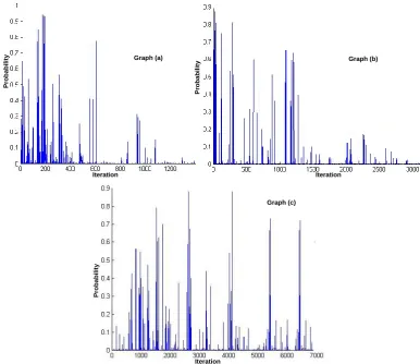
Figure ‎4-1: Transition probability of; graph (a) Geometric SA, graph (b): Dowsland‘s SA and graph (c): Azizi and Zolfaghari‘s SA ... 41

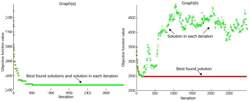
Figure ‎4-2: Progress of ASA, graph (a): (𝜆 = 𝑇_𝑚𝑖𝑛 = 1) and graph (b): (λ = 𝑇_𝑚𝑖𝑛 = 100) ... 43

Figure ‎4-3: New inventory diagram ... 44

Figure ‎4-4: An example of searching sequence ... 51

Figure ‎4-5: Percentage of optimality gap for different problem sizes ... 53

Figure ‎5-1: A main sequence (S) and different types of subtours (A, B, C, D) ... 61

Figure ‎5-2: Example (1) lot crossover ... 64

Figure ‎5-3: Node flow modelled by constraints (5-12) and (5-13) ... 65

Figure ‎5-4: An k-walk from 𝑝_𝑡𝛼 crossover product to product k ... 67

Figure ‎5-5: The k-walk from 𝑝_𝑡𝛼 much reach product k (if and only if 𝑧_𝑘𝑡𝑏𝑖𝑛 = 1) .... 69

Figure ‎5-6: The k-walk from 𝑝_𝑡𝛼 to k only traverse those product i for which 𝑧_𝑘𝑡𝑏𝑖𝑛 = 1 (and if and only if 𝑧_𝑘𝑡𝑏𝑖𝑛 = 1) ... 69

Figure ‎5-7: The k-walk from 𝑝_𝑡𝛼 must stop at product k (if and only if 𝑧_𝑘𝑡𝑏𝑖𝑛 = 1) ... 69

Figure ‎5-8: Production diagram of Example 2 obtained by Conventional, ML-SM and MLOV-SM models ... 72

Figure ‎5-9: Production diagram of Example 3 obtained by Conventional, ML-SM and MLOV-SM models ... 73

Figure ‎5-10: The production diagrams of 1L-PM, ML-PM and MLOV-PM ... 80

(7)

vii

List of Tables

(8)

1

Chapters:

1.

Introduction

Chapter 1

Introduction

1.1

Motivation

The increasing intensity of competition in global market leads manufacturing companies to become more efficient. A key success factor in achieving this is having an elaborate production planning system. Due to rapid growth in their size and complexity, the mathematical modelling and optimization of manufacturing systems is an important challenge for Operational Research (OR). This work focuses on two important challenges in managing a flexible flow line, namely the sizing and scheduling of production lots.

The flexible flow line also commonly referred to as hybrid flow shop, is a very prevalent production system and can be found in a vast number of industries, such as automotive, chemical, electronics, steel making, pharmaceutical, food and textile. FFL is a flow line with several parallel machines on some or all production stages and all products follow the same linear path through the system (Quadt, 2004).

Lotsizing and scheduling are closely interrelated and considerably combined in the literature for single machine production system. However, it can be more complicated and challenging to integrate both problems in complex production systems like FFLs. Quadt and Kuhn (2005) explicitly identified a lack of literature not only on combined lot sizing and scheduling but also on stand-alone lot sizing in FFLs. They presented an integrative solution approach for the combined lot-sizing and scheduling problem in FFLs which is limited to necessity of bottleneck stage identification.

(9)

2

procedure, possibly because the authors themselves recognized that the model‘s

complexity limits optimal solutions to just small instances. Recently, Mohammadi and Jafari (2010) developed an MIP (Mixed Integer Programming) model for flexible flow shop system based on Fandel and Stammen-Hegene (2006) formulations. They assumed the vertical interaction or ―inter-level synchronization‖ between production stages means a production on a production stage can only begin if there is sufficient amount of the product from the previous production stage. The shortage and lot-splitting are not allowed and sequence-dependent setup costs and times are triangles.

For the first time, in this thesis I research new challenges such as lot splitting and shortages, the practiced assumptions in flexible flow shop manufacturing systems (Özdamar and Barbaroso lu, 1999). Moreover sequence-dependent setup times can be ―non-triangular‖ as is the case in many industries such as chemical,

pharmaceutical, food and oil as some contamination occurs between certain products. For example, a product𝑝 contaminates some other product 𝑟, but in order to decontaminate, either an additional cleaning operation must be done as part of a substantial setup time setup𝑠𝑡_𝑝𝑟 that consumes the scarce production time, or a third product 𝑞 that can absorb the contamination must be produced. Such intermediate ―cleansing‖ or shortcut products can cause non-triangular setup times i.e. product𝑞’s

ability to absorb 𝑝’s contamination presents a shortcut opportunity and could result in shorter non-triangular setup times such that 𝑠𝑡_𝑝𝑟 > 𝑠𝑡_𝑝𝑞 + 𝑠𝑡_𝑞𝑟 and product q

cleans the machines whilst being processed.

Furthermore the ―lead-time synchronization‖ between production stages is assumed, means a product which is produced at a stage is available for production at the next stage only in the next periods.

(10)

3

FFL-FM) for GLSP-FFL and presented in 7th international industrial engineering conference 2010 (Mahdieh et al., 2010). Later, it was published in Journal of Industrial and Systems Engineering (Mahdieh et al., 2012). The first model (FFL-FS) is ―dynamic‖ since a decision variable appears as an upper limit index in many constraints, so the model cannot be solved as a MIP, whereas the second and third can. The efficiency of two latter MIP models was assessed and evaluated using numerical tests.

In this thesis, I present a new linear MIP model (FFL-ATSP) through adaption of Asymmetric Travelling Salesman Problem (ATSP) and show through the numerical tests that the new ATSP adaptation for GLSP-FFL has significant improvement of problem‘s solution in comparison with FFL-CC and FFL-FM.

Fleischmann and Meyr (1997) have showed that the General Lot sizing and Scheduling Problem (GLSP) for single machine with non-zero minimum lot sizes is a very difficult combinatorial problem and even finding a feasible solution is NP-complete. Thus, it can be concluded that the feasibility of our problem, the GLSP with non-zero sequence-dependent setup times/costs in a complex production system, flexible flow line, is also NP-complete. Hence it is necessary to develop an efficient solution procedure for GLSP-FFL. Here an Adaptive Simulated Annealing (ASA) with four well-organized initial solutions is designed to solve GLSP-FFL.

The main restriction of conventional ATSP based models is allowing one lot per product per periods so multiple lots of shortcut products cannot be produced per period when non-triangular setup exits. In a very recent work, Clark and I modelled multiple lots per period via different subtour elimination constraints for single machine and presented in 43rd Annual Symposium of the Brazilian Operational Research Society (Clark and Mahdieh, 2011) and its revision has been submitted to the International Journal of Production Research (Clark et al., 2012). In chapter 4 its extension to parallel machine and FFL system while incorporating all features of setup carry-over and setup-overlapping is modelled.

1.2

Characteristics of the Problem

(11)

4

inventory, backorder and production setup costs. The following system characteristics are explicitly noted:

The production line consists of several processing stages in series, separated by finite intermediate buffers, where each stage has one or more parallel identical machines. Multiple products can be produced at stages and production at each stage involves unrelated parallel machines with different production rates. All machines can produce any product. The available capacity of each machine is limited and can vary between periods and stages.

The finite planning horizon is divided into T macro-periods. The independent demand for all products is felt at the final stage at the end of each macro-period. It is known with certainty, but varies dynamically over the planning horizon. Demand for items in other stages is dependent on the production of the next stage. Backlog shortages are permitted for products at the final stage but are upper-bounded by a given percentage of demand in each macro-period. This is the practiced assumption in flow shop manufacturing systems (Özdamar et al., 1999).

The products may be manufactured in lots of varying size on any one of the parallel machines in each stage. The production rate can vary between products and machines, but is constant over the planning horizon. A changeover from one product to another requires a setup time during which the machine is unproductive. Setup times and costs are sequence dependent and can vary between machines. The setup state is conserved when no product is being processed (setup carryover). At the beginning of the planning horizon, each machine is setup for a specified product.

(12)

5

1.3

Outline of the chapters

The work is divided into six chapters. The reminder of the thesis is as follows. Chapter 2 provides the review of the literature and recent developments of deterministic dynamic lotsizing problems. The focus of this review is on capacitated lotsizing with sequence-dependent setup which is closely interrelated to scheduling and considerably combined in the literature. However, it can be more complicated and challenging to integrate both problems in complex production systems like FFL. This review discusses a modelling perspective of this challenge on a variety of machine configurations and points out fertile opportunities for future research.

Chapter 3 presents a novel linear MIP model (FFL-ATSP) for the problem of integrating lot sizing, loading, and scheduling in capacitated flexible flow lines with sequence-dependent setups through adaptation of ATSP. In comparison to our former models (CC and FM), fewer variables and constraints of FFL-ATSP model makes it more efficient and faster to be solved. Computational tests demonstrate the superiority of FFL-ATSP and its fast speed of solution compared to FFL-CC and FFL-FM.

Chapter 4 is devoted to heuristic solution procedure called an Adaptive Simulated Annealing (ASA) with an effective adaptive temperature control scheme for solving large instances in GLSP-FFL. The adaptive temperature control scheme changes temperature based on the number of consecutive improving moves and maintains it above the minimum level. Four initial solutions and neighbour operators are designed for ASA. The third and fourth novel initial solutions are obtained by solving well-organized model which extracts from the GLSP-FFL and ATSP model respectively. The numerical test compares the efficiency of different initial solutions.

Chapter 5 is presented the new mix integer programming formulations for capacitated lot sizing and scheduling with non-triangular and sequence-dependent setup times and costs incorporating all necessary features of setup carryover and overlapping on different machine configurations. The innovation of the new formulation is the modelling of non-triangular sequence-dependent setups within lot sizing model based on ATSP problem that allows multiple lots per product per period with polynomial number of disconnected subtours prohibition constraints.

(13)

6

inventory, three models including one-Lot (1L), Multiple Lots (ML) and Multiple Lots with setup overlapping (MLOV) are compared for three production systems: Single Machine (SM), Parallel Machines (PM) and FFL.

Finally, Chapter 6 summarizes the work and suggests directions for future research.

(14)

7

2.

Literature review

Chapter 2

Literature review

Generally, production planning in manufacturing determines what product is to be produced on which machine at what time. Production planning problems are typically classified according to hierarchical structure of long-term or strategic, medium-term or tactical and short-term or operational (Bitran and Tirupati, 1993). Long-term planning uses aggregated demand forecasts and makes strategic decisions such as aggregate resource planning to mainly achieve financial targets. Medium-term planning is more detailed and uses partially disaggregated demand to often determine Material Requirement Plan (MRP) and production quantities over planning horizon to optimize both operational and financial criteria while satisfying capacity limitations. Short-term planning uses totally disaggregated or actual demands to make day-to-day decisions on lot sizing, scheduling and loading problems (Heizer and Render, 2004, Karimi et al., 2003). Firstly, Gelders and Van Wassenhove (1981) gave an overview on medium- and short-term production planning and then in (Gelders and Van Wassenhove, 1982) they focused on the issue of integrating various decision level in hierarchical planning. So far considerable amount of research has been done on the various aspects of production planning and inventory management and large amount of models and techniques are already available (Graves et al., 1993, Pochet and Wolsey, 2006, Quadt and Kuhn, 2008, Silver et al., 1998, Thomas et al., 1993, Vollmann et al., 1997).

(15)

8

2.1

Basic Lotsizing models

Lot sizing aims to determine the optimal timing and level of production. Research on lot sizing started with the economic order quantity (EOQ) model (Harris, 1913). The main assumption for the EOQ models is constant demand for a product over an infinite planning horizon. Since there is no capacity constraint during a single level production process in the EOQ model, the economic lotsizing problem (ELSP) model is developed for multi-product or multi-item considering capacity constraint (Elmaghraby, 1978, Zipkin, 1991). However both EOQ and ELSP are based on a constant demand over an infinite time. The Wagner–Whitin (WW) model (Wagner and Whitin, 1958) is one of the first models for a dynamic demand where a finite planning horizon is subdivided into several discrete periods and demand is given per period and may very over time. The WW problem is single-level, single-item without capacity constraints. The capacitated lotsizing problem (CLSP) can be considered as the extension of the WW problem to capacity constraints and multi-item problem (Bitran and Yanasse, 1982, Haase, 1996, Karimi et al., 2003).

(16)

9

scheduling problem (GLSP) is a large bucket problem where due to simultaneously determine lot sizes and sequences, the planning periods divide into a predetermined number of (small bucket) micro-periods with at most one setup (Fleischmann and Meyr, 1997).

Several features or assumptions can be taken into account within the basic lot sizing models such as backlogging, sequence-dependent setup cost or/and time, setup carry over, setup overlapping and different machine configurations like single or parallel machine and single or multi stage. Therefore the numerous extensions of basic models and solving algorithms can be found in the literature. Furthermore there are excellent review papers on these extensions which are worthwhile to discuss here.

2.2

Previous reviews

Firstly Bahl et al. (1987) classified lot sizing models into four categories based on demand type including single- and multi-level, and presence or absence of resource constraints. Wolsey (1995) and Brahimi et al. (2006) focused on single item lot-sizing problem and discussed different extensions of this problem for real-world applications. Potts and Van Wassenhove (1992) reviewed the literature on the integration of lot sizing and scheduling from a scheduling perspective and pointed out the lack of work on combining lot sizing and scheduling. Later Drexl and Kimms (1997) gave an overview on lotsizing and scheduling models. They explained the differences of mathematical formulations for CLSP, DLSP, CSLD, PLSP and GLSP and also reviewed the extension of these models for multi-level structure. They underlined the importance of the extensions on sequence-dependent setup time, backlogging and parallel machines for future research. Karimi et al. (2003) discussed single-level lot sizing problem in both capacitated and uncapacitated cases and classified the literature based on different solution approaches applied for CLSP. They concluded similarly to Drexl and Kimms (1997) that there has been little literature regarding problems such as CLSP with backlogging or with setup time and setup carryover.

(17)

10

discussed the integration of these models with lot sizing problems and emphasized that most research has been done on single-machine configuration rather than other configurations. In an outstanding review Jans and Degraeve (2007b) gave an extensive overview of modelling deterministic single-level dynamic lotsizing problems and discussed the solution approach in Jans and Degraeve (2007a). They organized the extensions of these models in two directions. The first direction focuses on operational aspects including setups, production characters, inventory, demand side and rolling horizon. The second direction is towards more tactical and strategic aspects such as integrated production-distribution planning or supplier selection. They indicated that with introduction of sequence-dependent setups boundaries between lot sizing and scheduling are fading. They also noted that further integration of lot sizing, sequencing and loading (for example on parallel machine) is a challenging area for future research.

Quadt and Kuhn (2008) present a literature review on CLSP problems that incorporate one of the following extensions in the: back-orders, setup carry-over, sequencing, and parallel machines. Buschkühl et al. (2010) reviewed different modelling and algorithmic solution approaches for the multi-level capacitated lot-sizing problem (MLCLSP) while ignoring the sequencing and scheduling aspects.

2.3

Capacitated Lot Sizing and scheduling with

sequence-dependent setups

(18)

11

A further step for capacitated lot sizing is to determine a sequence for all products within a time period certainly if setup times or costs are sequence-dependent. One of the first studies regarding sequence-dependent setup cost is DLSPSD (DLSP with sequence-dependent setup cost) by Fleischmann (1994). He reformulated DLSPSD as Travelling Salesman Problem With Time Windows (TSPWTW) formulation to propose a heuristic solution. Salomon (1997) incorporated sequence-dependent setup time into DLSPSD by applying the same TSPWTW approach. The main serious restriction of DLSP as a small bucket is not allowing setup time to be fraction of period capacity.

(19)

12

approach to GLSP, Clark and Clark (2000) designed a mixed integer programming (MIP) model for simultaneous sequencing and lot sizing production lots on a set of

parallel machines. They assumed non-triangular sequence-dependent setup times, no setup cost and backlogging possibility.

(20)

13

2.4

Capacitated lot sizing and scheduling on different machine

configurations

Fading boundaries between lotsizing and scheduling poses special challenges for integrating lotsizing, sequencing and loading decisions on a variety of machine configurations. Machine configuration includes single machine, parallel machines, flow shop, flexible flow shop and job shop system. Most research has been focused on combing lotsizing and scheduling for the single machine configuration and research on other configurations is sparse.

Table ‎2-1: Literature review of capacitated big bucket lot sizing models with respect to back-orders, setup carry-over, sequencing on different machine configuration excluding single-machine. X: covered in reference; (X) partly covered in the reference.

References

Back-orders Setup times Setup carry-over

Sequencing Machine configuration

Over-time

Multi-level Dillenberger et al. (1993)

and (1994)

X X Parallel machine

Gopalakrishnan et al. (1995)

(X) X Parallel machine

Derstroff (1995) X Job shop X

Hindi (1995) Parallel machine

Özdamar and Birbil (1998)

X Partly Parallel

machine

X

Özdamar and Barbarosolu (1999)

X X Multi-stage with

identical parallel machine

X X

Kang et al.(1999) X X Parallel machine

Clark and Clark (2000) X X X X Parallel machine

Belvaux and Wolsey (2000)

X X Multiple machine X

Meyr (2002) X X X Parallel machine

Stadtler (2003) X Multiple machine X X

Quadt (2004) X X X Flexible flow line

Fandel and Stammen-Hegene (2006)

X X X Job shop X

Quadt and Kuhn (2009) X X X Parallel machine

Mahdieh et al.(2010) X X X X Flexible flow shop

Mohammadi et al (2010a), Mohammadi (2010b), (2010c) and Mohammadi and Ghomi (2011)

X X X Flow shop X

Mohammadi (2010) and Mohammadi and Jafari (2010)

X X X Flexible flow shop X

James and

Almada-Lobo (2011)

X X X Parallel machine

(21)

14

sequencing or parallel machines. They indicated that only Meyr (2002) and Kang et al. (1999) combined sequencing and lotsizing on parallel machines.

This thesis updates the literature review of capacitated lot sizing not only on parallel machines but also on multi-stage production system given in table 1. Stand alone capacitated lotsizing on parallel machines has been studied by Dillenberger et al. (1993) and (1994), Gopalakrishnan et al. (1995), Hindi (1995), Özdamar and Birbil (1998), Belvaux and Wolsey (2000), Stadtler (2003) and Quadt and Kuhn (2009).

Kang et al.(1999), Clark and Clark (2000), Meyr (2002) and James and Almada-Lobo (2011) integrated lotsizing and scheduling on parallel machines with different extensions as shown in table 2-1.

Moreover some recent work inspired by a specific real-world problem addresses capacitated lotsizing and scheduling on different machine configurations (Almada-Lobo et al., 2010, Almada-(Almada-Lobo et al., 2008, Almeder and Almada-(Almada-Lobo, 2011, Ferreira et al., 2012, Ghosh Dastidar and Nagi, 2005).

Flexible Flow Lines (FFL) are flow lines with parallel machines on some or all production stages and occur in many different environments, including automobile manufacture and printed circuit board manufacture (Kurz and Askin, 2003). The survey by Linn and Zhang (1999) reviewed the state of FFL scheduling research and

described a variety of different configurations. They noted the lack of research on

FFLs with more than two stages and the extensive using of dispatching rules in

practice. Their survey did not include any research or mention of lot sizing and scheduling within FFLs. Six years later, Quadt and Kuhn (2005) explicitly identified

a lack of literature for lot sizing and scheduling in FFLs and went on to describe a

hierarchical 3-phase approach consists of bottleneck planning, schedule roll out and product-to-slot assignment for integrative lot-sizing and scheduling. The second phase consisted of capacitated lot-sizing problem (CLSP) model (Bitran and Yanasse,

1982) generalised to the sequencing of lots of product families lot, the possibility of back-orders and parallel machines. While more general than needed for FFLs, the approach of Quadt and Kuhn (2005) is limited partly due to its aggregation of products into families, but primarily because of the necessity of bottleneck stage identification and stability during the planning run.

(22)

15

procedures (excluding lot-sizing), classifying them by general solution approach. They concluded by noting again that very little research has been published combining both lot sizing and scheduling in FFL, although in the same year Quadt

and Kuhn (2007a) did deal with batch scheduling.

Even research on stand-alone lot sizing for FFL is very limited. Derstroff (1995) considered a multi-level job shop problem and extended to include alternative routing on parallel machines where FFL can be interpreted as a special case of such a system. Özdamar and Barbarosolu (1999) considered the lotsizing problem for FFLs called the multi-stage capacitated lot sizing and loading problem (MCLSLP).

Relevant to the sequential stages of FFLs, Fandel and Stammen-Hegene (2006)

formulated the Multi Level General Lot sizing and Scheduling Problem with Multiple Machines (MLGLSP-MM), based on the GLSP for single level production and parallel machines. However, the paper contains only a mathematical model which is not a MIP since a variable is used as an index limit and also without any numerical tests or solution procedure, possibly because the authors themselves recognized that the model‘s complexity limits optimal solutions to just small instances. To recall, a

Mixed Integer Programming (MIP) is the optimization of a linear objective function subject to linear constraints in which some or all of the variables are restricted to be integers. In many settings the term refers to Mixed Integer linear programming (MILP).

(23)

16

stage can only begin if there is sufficient amount of the product from the previous production stage. The shortage is not permitted and sequence-dependent setup costs and times are triangles (i.e. it is never faster to change over from one product to another by means of a third product). Furthermore at stages with more than one machine, each product is produced entirely on one machine (lot splitting is not allowed).

Clark, Bijari and I extended MCLSLP to General Lot sizing and Scheduling in FFL (GLSP-FFL) which determines both lot sizes and sequences on parallel machines in multi-stage production system (Mahdieh et al., 2010, Mahdieh et al., 2012). However in contrast of MCLSLP the lot-splitting was allowed due to give more flexibility in the system through lot sequencing. The shortage was permitted and sequence-dependent setup costs and times could be ―non-triangle‖. Three models were presented (FFL-FS, FFL-CC and FFL-FM) based on Fandel and Stammen-Hegene (2006), Clark and Clark‘s (2000) and Fleischmann and Meyr (1997) sequencing formulation technique. It was also assumed the ―lead-time synchronization‖ between production means a product which is produced at a stage is available for production at the next stage only in the next period.

(24)

17

2.5

Conclusion and final remarks

This literature review focuses on modelling perspective of dynamic deterministic capacitated lot sizing problems (i.e. demands are known with certainty but may vary over time) with sequence dependent setup. The numerous extensions of the basic lotsizing models as Jans and Degraeve (2007b) cited nearly 250 references show that it can be applied to a variety of real-world industrial problems.

According to time structure capacitated lot sizing problems mainly are classified into small bucket (small time window) and big bucket (big time window) (Eppen and Martin, 1987, Gupta and Magnusson, 2005). Introducing sequence dependent setup leads lot sizing models to necessarily incorporate more scheduling aspects. Hence, fading boundaries between lotsizing and scheduling poses special challenges for integrating lotsizing, sequencing and loading decisions on a variety of machine configurations. The big bucket capacitated lotsizing is more flexible at integrating of lot sizing and scheduling decisions. Therefore GLSP (Fleischmann and Meyr, 1997) has been known as the most flexible simultaneous lotsizing and scheduling model in large bucket for representing different environment.

The adaptation of Asymmetric Travelling Salesman Problem (ATSP) is an alternative approach for lotsizing and scheduling with sequence dependent setup (Almada-lobo et al., 2007, Clark et al., 2010). Clark et al. (2010) showed that ATSP approaches were competitive with GLSP ones. Computationally comparing GLSP approach with different ATSP approaches based on a variety of subtour elimination method is another research opportunities to explore.

(25)

18

(26)

19

3.

Lot sizing and scheduling in FFL

Chapter 3

Lot sizing and scheduling in FFL

Fading boundaries between lotsizing and scheduling poses special challenges for integrating lotsizing, sequencing and loading decisions on a variety of machine configurations. Most research has been focused on combing lotsizing and scheduling for the single machine configuration and research on other configurations is sparse. In 2010, Clark, Bijari and I presented three different mathematical models to consider General Lotsizing and Scheduling Problem in Flexible Flow Line (GLSP-FFL) simultaneously (Mahdieh et al., 2010, Mahdieh et al., 2012). The first model, FS, cannot be solved as a MIP, whereas the second, CC, and third, FFL-FM, can. However due to complexity of GLSP-FFL, none of the MIP models could find optimal solution even for small problems and terminated with large value of optimality gap. In this chapter the novel linear MIP model through adaption of Asymmetric Travelling Salesman Problem (ATSP) is presented which makes an enormous reduction in number of variables and constraints and becomes much faster in comparison with the previous ones. Computational experiments are reported.

3.1

Problem definition

(27)

20

One of the most important interdependencies which makes the integrating of these two models crucial is the relationship between lot sizing and scheduling when setups are sequence dependent. In a lotsizing model, the optimal lot sizes are determined in order to minimise setup, holding and in some cases backorder costs. In the case of sequence dependent setups, the minimum-cost lot sizes also depend on the schedule on the machine since it influences the machine capacity.

This chapter presents three mathematical models with practical assumptions for simultaneous lotsizing and scheduling in one of the complex production systems called a flexible flow line.

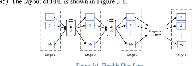
Flexible Flow Line (FFL) is a very prevalent production system which has extensive real-world applications in industry especially automotive, chemical, electronics, steel making, food, paper, pharmaceutical and textile (Linn and Zhang, 1999). A flexible flow line or hybrid flow shop can be considered as an extension of two classical systems, namely the flow shop and the parallel shop. The production line consists of several processing stages in series, separated by finite intermediate buffers, where each stage has one or more parallel identical machines (Pinedo, 1995). The layout of FFL is shown in Figure 3-1.

Stage 1 1

2

M1

Stage 2 1

2

M2

Stage 3 1

2

M3

Stage E 1

2

ME

B

u

ff

e

r

B

u

ff

e

r

[image:27.595.127.468.408.523.2]

Stages and Buffers

Figure ‎3-1: Flexible Flow Line

(28)

21

periods and stages. The finite planning horizon is divided into T macro-periods. The independent demand for all products is felt at the final stage at the end of each macro-period. It is known with certainty, but varies dynamically over the planning horizon.

The main assumptions of the problem were described in the following:

-Demand for items in other stages is dependent on the production of the next stage.

-Backlog shortages are permitted for products at the final stage and also are upper-bounded by a given proportion of demand (BP) in each macro-period for adding more flexibility to the production system. This is the practiced assumption in flow shop manufacturing system and is consistent with literature (Özdamar and Barbaroso lu, 1999). The backlog policy is appropriate in some situations and it can be other situations where we do not want to impose that. For example some products are more important than others so backlogs are allowed for them (by considering 𝐵𝑃 = 1) and not for the others (by considering 𝐵𝑃 = 0).

-The products may be manufactured in lots of varying size on any one of the parallel machines in each stage.

-The production rate can vary between products and machines, but is constant over the planning horizon.

-A changeover from one product to another requires a setup time during which the machine is unproductive. Setup times and costs are sequence dependent and can vary between machines.

-The setup state is conserved when no product is being processed.

-At the beginning of the planning horizon, each machine is setup for a specified product.

-A two-level time structure is assumed. Each macro-period consists of a variable number of periods with variable length. Each machine has its own micro-period segmentation, i.e., the number of micro-micro-period can differ between machines. Micro-periods do not have to be of equal durations on the same machine.

-At the start of a micro-period, a machine is setup and then produces just one product until the end of the micro-period.

(29)

22

there will be at most one setup per product per macro-period on each machine and so the number of micro-periods on a machine will be at most the number of products.

-Lot-splitting is permitted at any stage, i.e., each product can be simultaneously produced on more than one machine at any given stage.

-In order to obtain viable schedules, ―lead-time synchronization‖ is assumed means that there is the lead time of one period between different production stages. In this case, a product which is produced at a stage is available for production at the next stage only in the next periods. However in some industries, assuming a lead time of period may be unrealistic and lead to inferior model solutions.

The parameters and indices are:

Number of total products i, j, k

𝐽

Number of different stages e E

Number of different machines 𝑚_𝑒 available for production at stage e (so that the total number of machines over all stages is 𝑀 = 𝑀_𝑒 _𝑒)

𝑀_𝑒

Number of macro-periods t in the planning horizon

𝑇

The number of micro-periods f in macro-period t on machine 𝑚𝑒 𝐹_𝑚𝑡

Note that in the definition of 𝐹_𝑚𝑡 above, to avoid notational clutter such as 𝐹_𝑚_𝑒_𝑡, the simple index m is used when strictly speaking the subscripted index 𝑚𝑒 should

have been used. Similarly, the simple index f will be used when strictly speaking the subscripted index 𝑓𝑚𝑒𝑡 should be used. From now on, this convention will be used so

that the subscripts e and t are implied wherever the indices m and f are used. Figure 3-2 illustrates the segmentation of macro-periods into micro-periods on a machine m at any stage e. Note how the varying lengths of macro-periods differ between macro-periods.

Macro-period t = 1 … Macro-period t = T

𝑓 = 1 𝑓 = 2 … 𝑓 = 𝐹𝑚1 … 𝑓 = 1 𝑓 = 2 … 𝑓 = 𝐹𝑚𝑇

Micro-periods f … Micro-periods f

Figure ‎3-2: Micro-period segmentation on a machine differs between macro-periods

The data required are:

Demand for product i realised at the end of macro-period t

𝑑_𝑖𝑡

Available capacity of machine m in macro-period t

𝐶𝑚𝑡

Time needed to setup on machine m from product i to product j

𝑠𝑡_𝑖𝑗𝑚

Cost needed to setup on machine m from product i to product j

(30)

23

Capacity (processing time) on the machine m required to produce a unit of product i

𝑏_𝑖𝑚

Cost of holding a unit of product i from period t to t+1 at stage e

𝑕_𝑖𝑡𝑒

Cost of backordering a unit of end-item demand for product i from period t to t+1

𝑔𝑖𝑡

Maximum permitted proportion of total end-item demand that can be backordered. In case of having different backlog policies for products, it can be setup for each product distinctively (𝐵𝑃𝑖).

BP

The product setup on machine m at the end of period 0, i.e., the starting setup configuration

𝑖0𝑚

Cost of producing one unit of product i on machine m

𝑃𝑖𝑚

Upper bound 𝐶_𝑚𝑡 𝑏_𝑖𝑚 on the quantity of product i produced in macro-period t on machine m

𝑈𝐵_𝑖𝑚𝑡

Lower bound on the quantity of product i produced in macro-period t on machine m

𝐿𝐵𝑖𝑚𝑡

The objective of all three models presented below is to minimise backorders, inventory and setup costs of producing the 𝐽 products over the 𝑇 macro-periods in the planning horizon.

3.2

FFL-CC

Clark and Clark (2000) developed a mixed integer programming model for the multi-product lot-sizing problem with sequence-dependent set-up times that allows multiple set-ups per planning period. In the first model, the setup constraints are based on Clark and Clark‘s (2000) formulation. The decision variables are:

Inventory level of product i in stage e at the end of macro-period t.

𝐼_𝑖𝑒𝑡

Backordered amount of end-product i at the last stage E at the end of macro-period t.

𝐵𝑖𝐸𝑡

Production quantity of product i on machine m in micro-period f.

𝑥_𝑖𝑚𝑓

Binary variable, = 1 if there is a changeover from product i to product j on machine m at the start of micro-period f , = 0 otherwise.

𝑦_{𝑖𝑗𝑚𝑓}

The objective function minimises backorders, inventory and setup costs:

(3-1)

𝑠𝑐_𝑖𝑗𝑚 𝑦_{𝑖𝑗𝑚𝑓}

𝑖𝑗𝑒𝑚𝑡𝑓

+ 𝑕_𝑖𝑡𝑒 𝐼_𝑖𝑒𝑡 𝑖𝑡𝑒

+ 𝑔_𝑖𝑡 𝐵_𝑖𝐸𝑡 𝑖𝑡

Note how the implied summation limits and indices e and t avoid notational clutter in the first term in expression (3-1). The full cluttered version would be:

(cluttered 3-1)

𝑠𝑐𝑖𝑗 𝑚𝑒

𝐹𝑚𝑡

𝑓_{𝑚 𝑒𝑡}=1 𝑇

𝑡=1 𝑀𝑒

𝑚𝑒=1 𝐸

𝑒=1 𝐽

𝑗 =1,𝑖≠𝑗 𝐽

𝑖=1

(31)

24

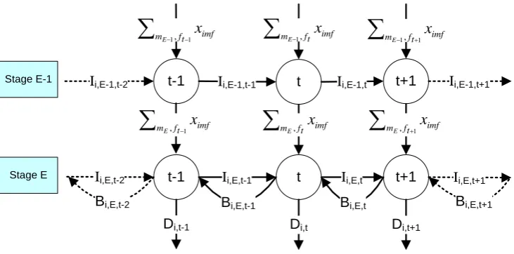
From now on, expressions will similarly be kept as concise as possible without sacrificing precision. Just occasionally, some clutter will be unavoidable, for example in constraints (3-3) and (3-9) below. If need be, production costs can be included in the objective function by appending the term 𝑖𝑒𝑚𝑡𝑓 𝑃𝑖𝑚 𝑥𝑖𝑚𝑓. Figure 3-3

shows the flow of production, inventory and backorders over different periods and stages. t-1 t-1 Di,t-1 t t Di,t t+1 t+1 Di,t+1 Ii,E,t-1

Ii,E-1,t-1 Ii,E-1,t

Ii,E,t

Ii,E-1,t-2

Ii,E,t-2

Ii,E-1,t+1

Ii,E,t+1

Bi,E,t-2 Bi,E,t-1 Bi,E,t Bi,E,t+1

Stage E-1

Stage E



mE ft imf

x

,

1



mE1,ft1 imf

x



 1,ft2 mE imf

x



mE1,ft_1 imf

x



mE,ft1 imf

x



t f mE imf

x

,



mE,ft1 imf

x



2 ,f_t mE imf

[image:31.595.152.501.204.371.2]

x

Figure ‎3-3: Flow diagram of GLSP-FFL

Constraints (3-2) and (3-3) follow from Figure 3-3:

∀ j, t (3-2)

𝐼_{𝑗𝐸 ,𝑡−1}− 𝐵_{𝑗𝐸 ,𝑡−1}+ 𝑥_𝑗𝑚𝑓 𝑚𝐸,𝑓𝑡

− 𝐼_𝑗𝐸𝑡 + 𝐵_𝑗𝐸𝑡 = 𝑑_𝑗𝑡

Constraint (3-2) expresses the material balance for end items, including backorders. Some clutter is required in order to be clear that the term 𝑚𝐸𝑓𝑥𝑗𝑚𝑓

refers only to the final stage E. However, note again how the implied use of the index 𝑓𝑚𝑒𝑡 in 𝑚𝐸𝑓𝑥𝑗𝑚𝑓 avoids further notational clutter. The context (∀ t) of (3-2)

makes it reasonable to assume that the values of f apply respectively to just the micro-periods within the specific macro-period t. The fully cluttered version would be:

𝑥_{𝑗 𝑚}_𝐸_𝑓_{𝑚 𝐸𝑡}

𝐹𝑚𝑡

𝑓_{𝑚 𝐸𝑡}=1 𝑀𝐸

𝑚𝐸=1

(32)

25

∀ 𝑗, 𝑡 𝑎𝑛𝑑 𝑒 = 1, … , 𝐸 − 1 (3-3)

𝐼𝑗𝑒 ,𝑡−1 + 𝑥𝑗𝑚𝑓 𝑚𝑒,𝑓𝑡

− 𝐼𝑗𝑒𝑡 = 𝑥𝑗𝑚𝑓

𝑚𝑒+1,𝑓𝑡+1

Constraint (3-4) bounds backorders of end items in any macro-period to be within a specified proportion of demand:

∀ i, t (3-4)

𝐵_𝑖𝑡𝐸 ≤ 𝐵𝑃 ∙ 𝑑_𝑖𝑡

Constraint (3-5) represents the limited capacity:

∀ 𝑒, 𝑚, 𝑡(3-5)

𝑠𝑡𝑖𝑗𝑚 𝑦𝑖𝑗𝑚𝑓 𝑖𝑗𝑓

+ 𝑏𝑖𝑚 𝑥𝑖𝑚𝑓 𝑖𝑓

≤ 𝐶𝑚𝑡

Constraints (3-6) and (3-7) specify the initial setup configuration in period one.

𝐿𝑚𝑡 refers to the first Micro-periods of period t on machine m.

∀ 𝑖 ≠ 𝑖_𝑜𝑚, 𝑗, 𝑒, 𝑚 (3-6)

𝑦_{𝑖𝑗𝑚 𝐿}_{𝑚 1} = 0

∀ , 𝑒, 𝑚 (3-7)

𝑦_𝑖_𝑜𝑚_{𝑗𝑚 𝐿}_{𝑚 1} 𝑗

= 1

Constraints (3-6) to (3-9) ensure that a setup on a machine in each micro-period may only occur between a single pair of different products.

∀ 𝑗, 𝑒, 𝑚, 𝑡 𝑎𝑛𝑑 𝑓 = 1, … , 𝐹_𝑚𝑡 − 1 (3-8)

𝑖

= 𝑦_{𝑗𝑘𝑚 ,𝑓+1}

𝑘

∀ 𝑗, 𝑒, 𝑚 𝑎𝑛𝑑 𝑡 = 2, … , 𝑇 (3-9)

𝑦𝑖𝑗𝑚 𝐹𝑚 ,𝑡−1 𝑖

= 𝑦𝑗𝑘𝑚 𝐿𝑚𝑡 𝑘

Constraint (3-10) enforces the appropriate setup before production:

∀ 𝑗, 𝑒, 𝑚, 𝑡, 𝑓(3-10)

𝑥𝑗𝑚𝑓 ≤ 𝑈𝐵𝑗𝑚𝑡 𝑦𝑖𝑗𝑚𝑓 𝑖

Constraint (3-11) enforces minimum lot sizes or specified lower bounds in order to avoid a setup change without subsequent production. If set-up costs or times do not satisfy the triangle inequality (𝑠𝑐_𝑖𝑗𝑚 + 𝑠𝑐_𝑗𝑘𝑚 ≥ 𝑠𝑐_𝑖𝑘𝑚 ∀𝑖, 𝑗, 𝑘, 𝑒, 𝑚), then (3-11) prohibits that a setup from i to k passes through a third product j without minimal production of j.

∀ 𝑒, 𝑚, 𝑡,j, f (3-11)

𝑥_𝑗𝑚𝑓 ≥ 𝐿𝐵_𝑗𝑚𝑡 𝑦_{𝑖𝑗𝑚𝑓}

𝑖≠𝑗

(33)

26

∀ 𝑗, 𝑒, 𝑚, 𝑡(3-12)

𝑦𝑖𝑗𝑚𝑓

𝑖,𝑓,(𝑖≠𝑗 )

≤ 1

∀ 𝑖, 𝑒, 𝑚, 𝑡(3-13)

𝑦𝑖𝑗𝑚𝑓

𝑗 ,𝑓,(𝑖≠𝑗 )

≤ 1

∀ 𝑖, 𝑒, 𝑚, 𝑡(3-14)

𝑗 ,𝑓,(𝑖≠𝑗 )

+ 𝑦_{𝑖𝑖𝑚 1}+ 𝑦_{𝑘𝑖𝑚𝐹} 𝑘

≤ 2

Constraints (3-12) and (3-13) ensure that there is at most one changeover from each product to a different one (𝑖 ≠ 𝑗). As shows in figure 3-4 Constraint (3-14) prohibits reproduction of a product which was the last product of the previous period (t-1) at the first and end of a current period (t).

A B C A

A D

t

[image:33.595.168.490.281.344.2]

t-1 t+1

Figure ‎3-4: Reproduction of the last product of the previous period t-1, at the first and end of a current period t.

Note that 𝐹_𝑚𝑡 is fixed by J, the number of products, therefore the number of setups may be less than J, but the remaining ones are treated as phantom setups from a product 𝑖 to itself (𝑦_{𝑖𝑖𝑚𝑓} = 1) with zero setup time (𝑠𝑡_𝑖𝑖𝑚 = 0) and no consequent production.

3.3

FFL-FM

Fleischmann and Meyr (1997)‘s adaptation of the General Lot sizing and Scheduling Problem (GLSP) to sequence-dependent setup times and parallel machines (Meyr, 2002) can be extended to the FFL. The parameters and continuous decision variables for this new model, denoted FFL-FM, are the same as for the FFL-CC model. However, to be consistent with Meyr‘s notation, the variable 𝑦_{𝑖𝑗𝑚𝑓} is renamed 𝑧𝑖𝑗𝑚𝑓, and y becomes a new setup-state variable as follows:

= 1 if machine m is setup for product i in the micro-period f, otherwise = 0.

𝑦_𝑖𝑚𝑓

= 1 if there is a setup changeover from product i to product j on machine

m at the start of micro-period f, otherwise = 0.

(34)

27

Note that there is no need to define 𝑧_{𝑖𝑗𝑚𝑓} a binary variable in the model since

𝑧𝑖𝑗𝑚𝑓 as a positive variable will take on the value 0 or 1 in any optimal solution

(Fleischmann and Meyr, 1997). As in model FFL-CC, the number 𝐹_𝑚𝑡of micro-periods within a macro-period is fixed at the number J of products and the objective function also minimises backorders, inventory and setup costs:

(3-15)

𝑠𝑐_𝑖𝑗𝑚 𝑧_{𝑖𝑗𝑚𝑓} 𝑖𝑗𝑒𝑚𝑡𝑓

Constraints (3-16) - (3-18) are identical to (3-2) - (3-4)of model FFL-CC .

∀ 𝑗, 𝑡 (3-16)

𝐼𝑗𝐸 ,𝑡−1− 𝐵𝑗𝐸 ,𝑡−1+ 𝑥𝑗𝑚𝑓 𝑚𝐸,𝑓𝑡

− 𝐼𝑗𝐸𝑡 + 𝐵𝑗𝐸𝑡 = 𝑑𝑗𝑡

∀ 𝑗, 𝑡 𝑎𝑛𝑑 𝑒 = 1, … , 𝐸 − 1 (3-17)

𝐼_{𝑗𝑒,𝑡−1} + 𝑥_𝑗𝑚𝑓 𝑚𝑒,𝑓𝑡

− 𝐼_𝑗𝑒𝑡 = 𝑥_𝑗𝑚𝑓

𝑚𝑒+1,𝑓𝑡+1

∀ 𝑖, 𝑡 (3-18)

Constraints (3-19) and (3-20) are (3-5) and (3-7) adapted to the new variables

𝑦𝑗𝑚𝑓 and 𝑧𝑖𝑗𝑚𝑓 :

∀ 𝑒, 𝑚, 𝑡 (3-19)

𝑠𝑡_𝑖𝑗𝑚 𝑧_{𝑖𝑗𝑚𝑓} 𝑖𝑗𝑓

+ 𝑏_𝑖𝑚 𝑥_𝑖𝑚𝑓 𝑖𝑓

≤ 𝐶_𝑚𝑡

∀ 𝑒, 𝑚, 𝑡 = 1 (3-20)

𝑧𝑖𝑜𝑚𝑗𝑚 1 𝑗

= 1

Note that this formulation has no strict equivalent of constraint (3-6) which states that the first setup in a macro-period t cannot be from a product which is not

𝑖𝑜𝑚. However, constraint (3-21) prohibits the value of 𝑦𝑖𝑚𝑓 from indicating that the

initial setup-state on a machine is any product which is not 𝑖_𝑜𝑚:

∀ 𝑖, 𝑒, 𝑚 𝑎𝑛𝑑 𝑡 = 1(3-21)

𝑦_{𝑖𝑚 1} ≤ 𝑧_𝑖_𝑜𝑚_{𝑖𝑚 1}

Constraint (3-22) imposes a minimum initial lot-size except for 𝑖𝑜𝑚:

∀ 𝑗 ≠ 𝑖𝑜𝑚 , 𝑒, 𝑚 𝑎𝑛𝑑 𝑡 = 1 (3-22) 𝑥𝑗𝑚 1 ≥ 𝐿𝐵𝑗𝑚𝑡 ∙ 𝑧𝑖𝑜𝑚𝑗𝑚 1

Constraint (3-23) is requires that a product can only be processed on a machine if it is setup for that product:

∀ 𝑒, 𝑚, 𝑗, 𝑡, 𝑓(3-23)

𝑥𝑗𝑚𝑓 ≤ 𝑈𝐵𝑗𝑚𝑡 ∙ 𝑦𝑗𝑚𝑓

(35)

28

∀ 𝑒, 𝑚, 𝑗, 𝑡, 𝑓 = 2, … , 𝐹_𝑚𝑡 (3-24)

𝑥_𝑗𝑚𝑓 ≥ 𝐿𝐵_𝑗𝑚𝑡 𝑦_𝑗𝑚𝑓 − 𝑦_{𝑗𝑚 ,𝑓−1}

∀ 𝑒, 𝑚, 𝑗, 𝑡 = 2, … , 𝑇 (3-25)

𝑥𝑗𝑚 1 ≥ 𝐿𝐵𝑗𝑚𝑡 𝑦𝑗𝑚 1− 𝑦𝑗𝑚 𝐹𝑚 ,𝑡−1

Constraint (3-26) ensures that only one setup state is defined in each micro period:

∀ 𝑒, 𝑚, 𝑡, 𝑓 (3-26)

𝑦𝑗𝑚𝑓

𝑗

= 1

Constraint (3-27) ensures that only one setup changeover occurs in each micro period:

∀ 𝑒, 𝑚, 𝑡, 𝑓 (3-27)

𝑧_{𝑖𝑗𝑚𝑓}

𝑖𝑗

= 1

Constraints (3-28) - (3-30) are (3-12) - (3-15) adapted to the new variable 𝑧_{𝑖𝑗𝑚𝑓}:

∀ 𝑗, 𝑒, 𝑚, 𝑡(3-28)

𝑧𝑖𝑗𝑚𝑓

𝑖,𝑓,(𝑖≠𝑗 )

≤ 1

∀ 𝑖, 𝑒, 𝑚, 𝑡(3-29)

𝑗 ,𝑓,(𝑖≠𝑗 )

≤ 1

∀ 𝑖, 𝑒, 𝑚, 𝑡(3-30)

𝑗 ,𝑓,(𝑖≠𝑗 )

+ 𝑧_{𝑖𝑖𝑚 1}+ 𝑧_{𝑘𝑖𝑚𝐹} 𝑘

≤ 2

Constraints (3-31) and (3-32) relate the setup state variables and changeover variables:

∀ 𝑒, 𝑚, 𝑖, 𝑗, 𝑡, 𝑓 = 2, … , 𝐹𝑚𝑎𝑥(3-31) 𝑧𝑖𝑗𝑚𝑓 ≥ 𝑦𝑖𝑚 ,𝑓−1+ 𝑦𝑗𝑚𝑓 − 1

∀ 𝑒, 𝑚, 𝑖, 𝑗, 𝑡 = 2, … , 𝑇(3-32)

𝑧𝑖𝑗𝑚 1 ≥ 𝑦𝑗𝑚 1+ 𝑦𝑖𝑚 𝐹𝑚 ,𝑡−1 − 1

3.4

FFL-ATSP

The Asymmetric Travelling Salesman Problem has been very extensively researched and can be adapted to model the problem of sequencing a set of lots with sequence dependent setups between them (Gupta and Magnusson, 2005). For example the CLSP with sequence-dependent setup times is related to the Travelling Salesman Problem (TSP) and the Vehicle Routing Problem (VRP) (Laporte, 1992a, Laporte, 1992b). Here, a novel MIP model is presented for GLSP-FFL via adaptation of ATSP.

The decision variables are:

Inventory level of product i in stage e at the end of macro-period t.

𝐼𝑖𝑒𝑡

Backordered amount of end-product i at the last stage E at the end of

(36)

29 period t.

Production quantity of product i on machine m in period t.

𝑥𝑖𝑚𝑡

Binary variable, = 1 if there is a changeover from product i to product j on machine m at the period t, = 0 otherwise.

𝑦_{𝑖𝑗𝑚𝑡}

Equals to 1 if product i is the setup state at the start of period t on machine m, otherwise = 0.

𝛼𝑖𝑚𝑡

Auxiliary variable to assign product i to machine m at period t.

𝑣𝑖𝑚𝑡

To avoid notational clutter, the simple index m is used when strictly speaking the subscripted index 𝑚_𝑒 except in some occasions, some clutter will be unavoidable. Note that the main novelty of ATSP adaptation is the elimination of the micro-period index 𝑓_𝑚_𝑒_𝑡 from changeover variables that causes the significant reduction in the number of binary variables in comparison with CC and FFL-FM. Thus, there is no need to pre-define a fix number of micro-periods in each period and assign products to them.

The objective function minimises backorders, inventory and setup costs:

(3-33)

𝑠𝑐_𝑖𝑗𝑚 𝑦_{𝑖𝑗𝑚𝑡} 𝑖𝑗𝑒𝑚𝑡

Constraints (3-34) and (3-35) express the material balance including backorders for end items and work in process respectively. Some clutter for m is required in order to be clear that the right-hand side refers to stages in both constraints:

∀ 𝑗, 𝑡(3-34)

𝐼𝑗𝐸 ,𝑡−1− 𝐵𝑗𝐸 ,𝑡−1+ 𝑥𝑗𝑚𝑡 𝑚𝐸

− 𝐼𝑗𝐸𝑡 + 𝐵𝑗𝐸𝑡 = 𝑑𝑗𝑡

∀ 𝑗, 𝑡 𝑎𝑛𝑑 𝑒 = 1, … , 𝐸 − 1(3-35)

𝐼𝑗𝑒 ,𝑡−1 + 𝑥𝑗𝑚𝑡 𝑚𝑒

− 𝐼𝑗𝑒𝑡 = 𝑥𝑗𝑚 ,𝑡+1 𝑚𝑒+1

Constraint (3-36) bounds backorders of end items in any macro-period to be within a specified proportion of demand:

∀ 𝑖, 𝑡 (3-36)

Constraint (3-37) represents the limited capacity:

∀ 𝑒, 𝑚, 𝑡 (3-37)

𝑠𝑡𝑖𝑗𝑚 𝑦𝑖𝑗𝑚𝑡 𝑖𝑗

+ 𝑏𝑖𝑚 𝑥𝑖𝑚𝑡 𝑖

≤ 𝐶𝑚𝑡

Constraint (3-38) indicates the first setup of each period which ensures that the machine is set up for exactly one product at the beginning of each period. The initial setup configuration at first period is expressed by constraint (3-39). Note that the

(37)

30

the first period and from constraint (3-40), it follows that 𝛼_𝑖𝑚𝑡 is an integer for i in the other periods. Finally constraints (3-38)-(3-40) enforce α_imt to be a binary variable.

∀ 𝑒, 𝑚, 𝑡(3-38)

𝛼𝑖𝑚𝑡

𝐽

𝑖=1

= 1

∀ 𝑒, 𝑚, 𝑡 = 1(3-39)

𝛼_𝑖_𝑜𝑚_𝑚𝑡 = 1

Constraints (3-38)–(3-41) entirely determine the sequence of products on a machine in each period and cause a setup carryover of the machine between periods.

∀ 𝑒, 𝑚, 𝑖 𝑎𝑛𝑑 𝑡 = 1 … , 𝑇 − 1(3-40)

𝛼_𝑖𝑚𝑡 + 𝑦_{𝑗𝑖𝑚𝑡}

𝑗

= 𝑦_{𝑖𝑗𝑚𝑡} 𝑗

+ 𝛼_{𝑖𝑚 𝑡+1}

∀ 𝑒, 𝑚, 𝑖 (3-40a)

𝛼_𝑖𝑚𝑇 + 𝑦_{𝑗𝑖𝑚𝑇}

𝑗

≥ 𝑦_{𝑖𝑗𝑚𝑇} 𝑗

To simplify constraints (3-40) and (3-40a) into a single constraint, it is considered that set 𝑡 = {1, . . , 𝑇 + 1} for the variable 𝛼_𝑖𝑚𝑡. Thus the constraint (3-40a) is cancelled and the domain of t in constraint (3-40) is changed to for all t(∀t).

Constraint (3-40) keeps a balanced network flow of the machine set up state and carries to next period. It means that if there is an input setup for product i

( 𝑦𝑗 𝑗𝑖𝑚𝑡 = 1) and no output setup ( 𝑦𝑗 𝑖𝑗𝑚𝑡 = 0) in period t then this setup is the

last one in period t and the machine carries the setup configuration of product i into the next period (𝛼_{𝑖𝑚 ,𝑡+1} = 1). On the other hand, if there is an output setup and no input setup, then the machine is configured for product i at the beginning of period t

(𝛼𝑖𝑚 ,𝑡 = 1). Moreover if no setup is performed in period t, then setup is carried to

the next period.

∀ 𝑒, 𝑚, 𝑖, 𝑗, 𝑡 (3-41)

𝑣𝑖𝑚𝑡 − 𝑣𝑗𝑚𝑡 + 𝐽 × 𝑦𝑖𝑗𝑚𝑡 ≤ 𝐽 − 1

Constraint (3-41) prohibits product subtours which is based on Miller, Tucker and Zemlin‘s (MTZ) subtours elimination constraint and it was originally proposed

(38)

31

vehicle routing problems. The MTZ‘s constraint is lifted by adding ( 𝐽 − 2) × 𝑦_{𝑗𝑖𝑚𝑡}

to the left hand side of the constraint:

∀ 𝑒, 𝑚, 𝑖, 𝑗, 𝑡 (3-41a)

𝑣_𝑖𝑚𝑡 − 𝑣_𝑗𝑚𝑡 + 𝐽 × 𝑦_{𝑖𝑗𝑚𝑡} + ( 𝐽 − 2) × 𝑦_{𝑗𝑖𝑚𝑡} ≤ 𝐽 − 1

Desrochers and Laporte (1991) compared the lifted MTZ formulation with the original formulation for different TSP and VRP problems, though the lifted MTZ formulation has shown low improvement in the case of Asymmetric TSP test problems. Similarly in this thesis, both constraints (MTZ constraint with and without lifting) will be tested for all the problems in the next section.

Constraint (3-42) enforces the appropriate setup before production, either at the beginning or within a period:

∀ 𝑒, 𝑚, 𝑗, 𝑡 (3-42)

𝑥_𝑗𝑚𝑡 ≤ 𝑈𝐵_𝑗𝑚𝑡 𝑦_{𝑖𝑗𝑚𝑡}

𝑖

+ 𝛼_𝑗𝑚𝑡

Constraint (3-43) enforces minimum lot sizes to avoid a setup change without subsequent production in case of non-triangle setup. Furthermore it does not enforce a minimum lot size to the product which already setup at the start of a period.

∀ 𝑒, 𝑚, 𝑗, 𝑡 (3-43)

𝑥_𝑗𝑚𝑡 ≥ 𝐿𝐵_𝑗𝑚𝑡 𝑦_{𝑖𝑗𝑚𝑡}

𝑖

− 𝛼_𝑗𝑚𝑡

3.5

Comparison of variables and constraints in FFL-CC, FFL-FM

and FFL-ATSP

The main difference between models FFL-CC and FFL-FM is the setup variables. As Clark and Clark (2000) did, the FFL-CC setups are modelled with just one set of binary variables, 𝑦_{𝑖𝑗𝑚𝑓}, whereas in the FFL-FM model setups are formulated with one set of binary variables 𝑦_𝑖𝑚𝑓 and one set of positive variables

𝑧_{𝑖𝑗𝑚𝑓} , similar to Fleischmann and Meyr (1997). However in FFL-ATSP, as a result

(39)

[image:39.595.104.562.93.221.2]

32

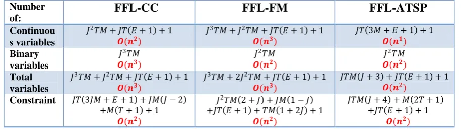
Table ‎3-1: Number of variables and constraints in FFL-CC , FFL-FM and FFL-ATSP

Number of:

FFL-CC FFL-FM FFL-ATSP

Continuou s variables

𝐽2_{𝑇𝑀 + 𝐽𝑇 𝐸 + 1 + 1}

𝑶(𝒏𝟐₎ 𝐽

3_{𝑇𝑀 + 𝐽}2_{𝑇𝑀 + 𝐽𝑇 𝐸 + 1 + 1}

𝑶(𝒏𝟑₎ 𝐽𝑇 3𝑀 + 𝐸 + 1 + 1_𝑶(𝒏𝟏₎

Binary variables

𝐽3_𝑇𝑀

𝑶(𝒏𝟑₎ 𝐽

2_𝑇𝑀

𝑶(𝒏𝟐₎ 𝐽

2_𝑇𝑀 𝑶(𝒏𝟐₎

Total variables

𝐽3_{𝑇𝑀 + 𝐽}2_{𝑇𝑀 + 𝐽𝑇 𝐸 + 1 + 1}

𝑶(𝒏𝟑₎ 𝐽

3_{𝑇𝑀 + 2𝐽}2_{𝑇𝑀 + 𝐽𝑇 𝐸 + 1 + 1}

𝑶(𝒏𝟑₎ 𝐽𝑇𝑀 𝐽 + 3 + 𝐽𝑇 𝐸 + 1 + 1_𝑶(𝒏2₎

Constraint 𝐽𝑇 3𝐽𝑀 + 𝐸 + 1 + 𝐽𝑀 𝐽 − 2

+𝑀 𝑇 + 1 + 1

𝑶(𝒏𝟐₎

𝐽2_{𝑇𝑀 2 + 𝐽 + 𝐽𝑀 1 − 𝐽}

+𝐽𝑇 𝐸 + 1 + 𝑇𝑀 1 + 2𝐽 + 1

𝑶(𝒏𝟐₎

𝐽𝑇𝑀 𝐽 + 4 + 𝑀 2𝑇 + 1 +𝐽𝑇 𝐸 + 1 + 1

𝑶(𝒏𝟐₎

FFL-ATSP has fewest constraints while the order of magnitude of the number of constraints is the same in all the three models. The computational tests in the next section will provide more insights into the relative efficiencies of the three models.

3.6

Experimental design

The aim of this section is to compare the novel linear MIP model FFL-ATSP with FFL-CC and FFL-FM through computational tests on small and larger problems. Özdamar and Barbarasoglu (1999) designed test problems to solve the CLSP in FFLs. Later Quadt(2004) also used their testing method. This thesis will do the same by varying the attributes of the problem data to test the performance of the models under different conditions. These attributes are conspicuously used in various lotsizing problems in the literature (Buschkühl et al., 2010) and tend to have a significant effect on solution quality.

The experimental design used the following factors: 1. Model formulation

2. Attribute and Dimensionality of Problem 3. Variability of demand

4. Inventory holding cost 5. Tightness of capacity

The problem parameters outside the statistical experimental design are randomly generated as follows: Processing times 𝑏_𝑖𝑚 (in hours) are generated from uniform distribution U(1,5) for all products i and machines m. Setup costs 𝑠𝑐_𝑖𝑗𝑚 are generated from U(300,500). Set-up times are related to the total processing time:

(3-44)

(40)

33

where 𝑆 is generated from U(0.05,0.10) and 𝑀𝑎𝑥𝑓𝑎𝑐 = 𝑚𝑎𝑥_𝑒{𝑀_𝑒} is the maximum number of machines at any stage. In the other words setup times are proportional to the mean production time per machine-period.

The factor levels within the experimental design are randomly generated as follows:

1. Model Formulation: FFL-ATSP, FFL-CC and FFL-FM

2. The attributes and dimensionality of Problem (discussed further below): a. Small: 𝐸 = 2, 𝑀_𝑒 = 2, 𝐽 = 4, 𝑇 = 6

b. Large: 𝐸 = 3, 𝑀_𝑒 = 3, 𝐽 = 8, 𝑇 = 6

3. Demand variability is either low, 𝑑𝑖𝑡 being generated from U(90,110), or high,

from U(50,150).

4. Holding and backordering costs assume that successive stages add value, so that work-in-process holding costs will increase as material progresses along the line. To reflect this, a value-added percentage factor 𝑉𝐴𝑃 is used, whose value is 1.1 (low) or 1.3 (high). Inventory costs are then generated consecutively as follows: The first stage‘s unit holding cost 𝑕_𝑖𝑡1 for product i is generated from U(1,20).

For subsequent stages, 𝑕_𝑖𝑡𝑒 = 𝑉𝐴𝑃 ∙ 𝑕_{𝑖𝑡 ,𝑒−1} for 𝑒 ≥ 2. The backordering cost for product i is 𝐵_𝑖𝑡 = 1.25 ∙ 𝑕_𝑖𝑡𝐸.

5. Capacity tightness is measured by a factor 𝐶𝐴𝑇 with value 1.2 (tight) or 1.6 (loose). The mean capacity requirement C per machine at each stage is calculated as:

(3-45)

𝐶 = 𝑚𝑎𝑥 𝑒

𝑏_𝑗𝑚 ∙ 𝑑_𝑗𝑡 𝑗𝑡𝑚

�