A Correlation-Test-Based Validation Procedure for
Identified Neural Networks
Li Feng Zhang, Quan Min Zhu, and Ashley Longden
Abstract—In this study, an enhanced correlation-test-based val-idation procedure is developed to check the quality of identified neural networks in modeling of nonlinear systems. The new com-putation algorithm upgrades the validation power by including a direct correlation test between residuals and delayed outputs that have been quoted indirectly in the most previous approaches. Fur-thermore, based on the new validation procedure, three guidelines are proposed in this study to help explain the validation results and the statistic properties of the residuals. It is hoped that this study could promote awareness of why the correlation tests are an effec-tive method of validating identified neural networks, and provide examples how to use the tests in user applications.
Index Terms—Correlation functions, model validation, neural networks, nonlinear dynamical systems, residuals.
I. INTRODUCTION
N
EURAL NETWORK (NN) has been extensively studiedand applied as a generic and powerful black-box mod-eling technique to enhance complex nonlinear system modmod-eling and identification [1]–[4]. In system identification procedure, validation is the final step to check the adequacy of identified models. Because an NN could be incorrectly designed due to many problems such as incorrect network selection, incorrect input vector selection, insufficient training, and overfitting, val-idation is a very important means to determine if the NN agrees sufficiently well with the observations. Generally, the basic sta-tistics of residuals, e.g., mean and variance or standard devia-tion, are considered to be critical indices for the identified NNs to check whether the residuals are reduced to the lowest possible levels. However, the levels of the residuals sometimes cannot clearly and directly indicate the adequacy of the identified NNs since the original systems are always contaminated in unknown noisy environments.
To properly validate linear and nonlinear models, several methods for model validation based on correlation tests have been developed that are based on the concept that if a model is valid, the residuals should be reduced to a white noise and uncorrelated to the delayed system inputs and outputs [5].
Manuscript received September 21, 2006; revised August 23, 2007 and April 04, 2008; accepted April 16, 2008. First published December 02, 2008; current version published January 05, 2009.
L. F. Zhang is with the Department of Economic Information Management, School of Information, Renmin University of China, Beijing, 100872, China.
Q. M. Zhu and A. Longden are with the Faculty of Computing, Engineering and Mathematical Sciences, University of the West of England, Bristol BS16 1QY, U.K. (e-mail: [email protected]).
Color versions of one or more of the figures in this paper are available online at http://ieeexplore.ieee.org.
Digital Object Identifier 10.1109/TNN.2008.2003223
For linear model validation, autocorrelation function (ACF) and cross-correlation function (CCF) have been successfully applied to detect the whiteness and randomness of the residuals [6]–[9]. For nonlinear model validation, several higher order correlation-test-based approaches have been developed for detecting the nonlinear correlationships between residuals and delayed residuals, inputs and outputs [10]–[16]. Recently, two sets of novel first-order correlation functions named combined omnidirectional autocorrelation function (ODACF) and com-bined omnidirectional cross-correlation function (ODCCF) have been proposed to detect nonlinear correlations between variables [17]. Then, they have been used to construct a set of new nonlinear model validity tests [18]. In comparison to pre-vious higher order correlation-test-based approaches, the new method provides an enhanced nonlinear correlation detection power and a condensed correlation illustration.
It should be mentioned that almost all previous validity tests only focus on the correlation computation for residuals and in-puts. In these methods, the correlation between residuals and delayed outputs is indirectly detected so that they sometimes display less detection power particularly when relatively large uncorrelated noise exists in the residuals. Moreover, since the previous methods do not individually detect all possible omitted regressors in residuals, they cannot provide a comprehensive in-dication of the statistics of the residuals. To overcome the prob-lems, the combined ODACF- and ODCCF-based model valida-tion method is further developed in this study and applied to check the quality of identified NNs. The purpose of the study is outlined as follows.
1) To provide an effective solution for neural network valida-tion. So far, most of the publications on the identification of NNs have only used the observation of residuals and its basic statistics (mean and variance) to check the goodness of the networks. As mentioned above, correlation tests can be used to indicate the accuracy of NNs. Without such tests, the performance of the identified NNs cannot be assured. 2) To develop a direct correlation test between residuals and
delayed outputs. This is the further expansion from the re-cent study [18]. In this study, a combined ODCCF test be-tween residuals and delayed outputs is proposed to upgrade the detection power. Furthermore, since the enhanced va-lidity tests individually and directly detect all the possible omitted regressors in residuals, they can provide a com-prehensive indication of the statistics of the residuals. A set of guidelines will be proposed to further explain the validation results and reveal the insufficiencies of invalid NNs. These guidelines can be used as a reference to sug-gest how to improve an invalid NN during the identification procedure.
3) To test the developed method with two simulated examples in neural network modeling of complex nonlinear systems. It is hoped that these two bench tests also can provide ex-amples for users considering applying this validation pro-cedure to their identified neural networks.
The rest of the study is organized as follows. In Section II, the principles of NN and nonlinear system identification are briefly explained to lay a basis for validating neural networks using cor-relation tests. In Section III, the new corcor-relation-based validity tests are developed with analytical proof and numerical demon-strations. In Section IV, two simulation examples are studied with neural network modeling of both nonlinear static and dy-namical systems. The identification and validation results are analyzed to demonstrate the effectiveness of the new validation procedure. In Section V, conclusions are drawn to summarize the study.
II. NEURALNETWORK, SYSTEMIDENTIFICATION ANDMODELVALIDATION
A. Neural Networks for System Identification and the Needs of Validity Tests
An NN is a massively parallel distributed processing para-digm made up of simple processing units (neurons) with highly interconnected by parameters (weights and biases), which are used to store acquired knowledge. Learning algorithms for jus-tifying the parameters with illustrative examples (training sets) are implemented to train the NNs to achieve acquired perfor-mance. For static modeling, various types of NNs, such as multi-layer perception (MLP, also referred to as feedforward network) networks, radial basis function (RBF) networks, have been de-veloped and successfully applied to map the linear and non-linear static relationships between the inputs and the outputs of the systems. For dynamic modeling, two main types of NNs have been widely studied, in particular, recurrent neural network that represents the dynamic behaviors by adding inner feedback loops to the neurons, and time delay neural network (TDNN) that uses the external time delay elements to perform temporal processing.
For the black-box modeling applications, the ultimate objec-tive of NN design is to find a network whose response matches the outputs of the underlying system for the given inputs. Finding a proper NN can be considered as a typical system identification problem. The major steps of identifying an NN to represent an underlying system are outlined in Fig. 1.
During the entire NN design procedure, various potential problems could result in an inadequate identification. Looking through the above NN training loop, the main problems are listed step by step.
Experimental design: This step involves a number of choices with regard to the system output signals to measure and the input signals to manipulate. It is important that testing signals and past system responses excite the system signifi-cantly in the region of the system space so that comprehensive modeling within this space is accomplished. These choices are mainly concerned with the prior knowledge of the underlying system but not the validity of the NN.
Data: Then, the data of the measured or simulated inputs and outputs are collected from the underlying systems. The main problem in aspect of validation is that the level of the actual noise, which is the unpredictable part of the measured data, is always unknown. The basic statistics of residuals, therefore, cannot be used to directly indicate the adequacy of the identified NN. For example, when large noise signals exist in measured outputs and inputs, the variance of residuals will maintain high level even though the NN is adequate. On the other hand, an NN with low-level residuals could be invalid while the level of the actual noise in contaminated data is comparatively low.
Setting up the NN: This step is concerned with the choice of the types of networks, number of layers and neurons, the input set of the network, and the initialization of the weights and bi-ases. Each type of NN has individual advantages and disadvan-tages for different applications. The number of layers and the number of neurons in each layer also significantly affect the ca-pability of the network. An oversimple NN structure will result in underfitting and an overcomplex NN structure can result in overfitting. This selection is equivalent to the model structure determination in terms of classical system identification. Fur-thermore, the selection of the input set that includes the delayed input and output signals is a crucial issue that could result in an insufficient lag terms or omission of input signals. Accordingly, in these circumstances, the system can never be identified prop-erly. This selection is equivalent to the variable and lag selection in terms of classical system identification. In other words, all these factors need to be determined properly to ensure that the NN can be used to adequately represent the underlying system.
Learning algorithm and training: NNs are trained through specified learning algorithms to obtain a set of weights and bi-ases to attain desired design objectives. Unsuitable initializa-tion, insufficient training iterations including local minimum problem, and too many training iterations with the resulting po-tential problem of overfitting (also related to network structure selection) will result in invalid networks. This training proce-dure is, respectively, equivalent to the parameter estimation in terms of classical system identification.
Network validation: Since many problems could result in an invalid NN identification, it is necessary to check the ade-quacy of the network representation before applying the NN in practice.
B. The Uncorrelated Properties of Residuals
To derive the new NN validity tests, the principles of identifi-cation and validation for a nonlinear dynamic system are briefly summarized as follows. Consider the general mathematical de-scription of nonlinear SISO system expressed as
(1)
of system (1) is NARMAX model (nonlinear autoregressive moving average with exogenous inputs) [19], [20], which has been extensively studied in nonlinear system identification. Alternatively, neural networks can be used to approximate the relationships between the data sequences observed from system (1). Then, the input set of the network to be identified is defined as follows [21]:
(2)
The one-step-ahead predicted outputs and residuals are ex-pressed as
(3) (4)
where and denote the predicted outputs and the resid-uals (also called prediction error), respectively, and denotes the identified nonlinear relationship, which is described by the trained network and used to approximate the behaviors of the underlying system. If the NN is adequate, the entire informa-tion contained in the input vector should be completely utilized to predict the outputs of the system. For a noise-free system,
therefore, and . A lower level of residuals
indicates a better identification.
For a noisy system, it has been commonly accepted that the predicted outputs obtained from using a valid NN should be the predictable part of the actual system outputs, and the resid-uals should be the unpredictable part of the outputs. Hence, if an NN is valid, the residuals should be reduced to a white noise sequence and random to all the NN inputs, expressed as where denotes an uncorrelated noise sequence with zero mean and finite variance. In contrast, if an NN is in-valid, the residuals should contain predictable information. In other words, the residuals should correlate to the delayed in-puts, outin-puts, and residuals. Then, the residuals for an invalid NN can be express as follows:
(5)
where is a linear or nonlinear relationship that needs to be superadded into the estimated relationship .
Since and is usually unknown in the real
applications, it is difficult to directly indicate the quality of the NN, e.g., proper fitted, overfitting, or underfitting, by just using the variance or standard deviation of the residuals.
III. CORRELATION-TEST-BASED NEURAL
NETWORKVALIDATION
To provide better solutions, ACF- and CCF-based linear model validation methods have been proposed to check if the residuals are correlated to delayed residuals, inputs, and outputs [6]–[9]. For nonlinear model validation, ACF and CCF are obviously insufficient since nonlinear terms may exist in residuals. To overcome this problem, several higher order cor-relation-based nonlinear model validation methods have been developed in the last three decades. These include multidimen-sional CCF and higher order CCF tests [10], [15], [22]–[24],
a combination of five first- and second-order ACF and CCF tests [11], higher order ACF and CCF between outputs, inputs, and residuals [13], [14], and multidirectional correlation tests [16]. In 2007, a set of new first-order correlation functions, ODCCFs, has been proposed and applied to cope with the prob-lems of nonlinear model validation [17], [18]. Compared to the previous methods, the new approach provides an enhanced nonlinear correlation detection power and a more condensed correlation illustration.
A. Combined ODACF and ODCCF Tests for Validation
ODCCFs can be generally expressed as follows [17]. Con-sider two data sequences and
(6)
(7)
(8)
(9)
where in (6)–(9) denotes that the mean level has been removed from the corresponding data sequence, and
(10)
Then, the results obtained using ODCCFs are combined to constitute a much condensed formulation to provide better il-lustration for detected correlations [17].
Definition [Combined ODCCFs ]: If
then
(11)
else
(12)
com-bined ODACF. Subsequently, a set of model validity-test-based combined ODACF and combined ODCCF have been proposed [18] and formulated as follows.
Combined ODACF validation of residuals
otherwise (13)
Combined ODCCF validation between inputs and residuals
(14)
and directly detect the correlations between residuals, delayed residuals, and inputs. In addition, the corre-lation between residuals and delayed outputs can also be indi-rectly detected by (13) and (14). Consider a single-input–single-output (SISO) dynamic system as
(15)
If the effect of exists in the residuals so that the identified model or network is inadequate, the residuals and
can be derived as
(16)
Since is in terms of both and ,
should be correlated to both and .
Consequently, and can be used to indicate the
correlation between and .
However, the indirect indication of the correlation between residuals and delayed outputs still has two drawbacks. First, the
correlation between and is indirectly computed as
and so that it sometimes displays less detec-tion power, practically, when the variance of
is much smaller than the variance of . Second, since the de-layed outputs are always used as crucial regressors in system identification, the omitted effects of delayed outputs in the resid-uals need to be detected clearly. A clear indication of the cor-relation between residuals and delayed outputs will provide the modeler or the network designer with further information about how to improve the performance of the model or the network. Moreover, all the previous approaches have the same problem since they all mainly concentrate on detecting the autocorrela-tion of residuals and the cross correlaautocorrela-tion between residuals and inputs.
B. The Enhanced Validity Tests
To provide a more comprehensive and effective detection, a direct correlation test between residuals and outputs is incorpo-rated into the validity tests. For a valid model or network, the residuals should be completely uncorrelated to the delayed out-puts at all the delay time instants except .
Fact: should be a nonzero number with absolute value smaller than 1, even though the network is valid. This is proved as follows.
Proof: Consider an identified NN expressed as (3) and (4). As formulated in (4), the relationship between and can be generally described as a linear combination. Hence, the relationship between and can be properly detected by CCF, which is the third function in ODCCFs. CCF
can be computed as follows:
(17)
where the bar on the variables denotes the mean value of the variables. When the identified network is valid, should be reduced to an uncorrelated noise sequence with zero mean and finite variance [11]. Then, is used to replace to yield
(18)
Since is uncorrelated to and , then
. Since , it gives
(19)
Then
(20)
Consequently, the enhanced validity tests are proposed as follows.
The enhanced validity tests:
Combined ODACF validation of residuals
Combined ODCCF validation between inputs and residuals
(22)
Combined ODCCF validation between outputs and residuals
otherwise. (23)
Remark: For a large data length , all the correlation func-tion estimates are asymptotically normal with zero mean and finite variance from the center limit theorem [25], which states that the sum of a large number independent and identically tributed random variables will be approximately normally dis-tributed. If the identified model is acceptable, the correlation functions should lie inside the 95% confidence interval, which
is from to .
Compared to the previous methods, the enhanced validity tests directly detect all the regressors that may exist in resid-uals so that they can provide a more comprehensive indication of the potential insufficiencies of invalid NNs. Three guidelines for distinguishing the potential problems of invalid NNs, which can be revealed through using the new validity tests, are pro-posed as follows.
Analysis of the validation results
1) While lies outside the confidence interval, the resid-uals can be primarily assumed as including omitted pre-dictable information in terms of delayed outputs.
2) While lies outside the confidence interval and lies inside the confidence interval, the residuals can be primarily assumed as including omitted predictable information in terms of delayed inputs.
3) While only lies outside the confidence interval, the residuals can be assumed as including correlated noise. If an identified NN is invalid because part of the correlation functions lie outside the confidence interval, after assuring the network is selected and trained properly, the NN can be im-proved based on these guidelines by involving more regressors into the network step by step. A simple example is employed to illustrate the new validity tests and the proposed guidelines. Consider a nonlinear system expressed as
(24)
The following five residual equations are possibly resulted from ill model structure selection or inadequately estimated model parameters:
(25)
where was the uniformly distributed random input
[image:5.594.335.518.61.288.2]se-quence with zero mean and amplitude from to . was
Fig. 1. Loop for identifying an NN.
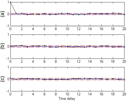
Fig. 2. Validity tests for" in (25): (a) (); (b) (); and (c) ().
the normally distributed random noise sequence with zero mean and variance of . All these data sequences have length of . Figs. 2–6, respectively, show the results obtained from using the new method for the five residual sequences in (25). In each figure, the dash lines indicate the confidence interval.
In Fig. 2, there is no correlation function that exceeds the con-fidence limits so is an uncorrelated residual. In Figs. 3–6, the correlations lie outside the confidence interval, so to are correlated residuals. As indicated in (25), all these four residual sequences include omitted predictable terms.
According to the three guidelines, the validation results can be extensively analyzed as follows. In Fig. 3, only ex-ceeds the confidence limits so that can be diagnosed as col-ored noise, which is correlated to the delayed residuals. Fig. 4, clearly shows that only lies outside the confidence in-terval that is correlated with the delayed inputs. In Fig. 5,
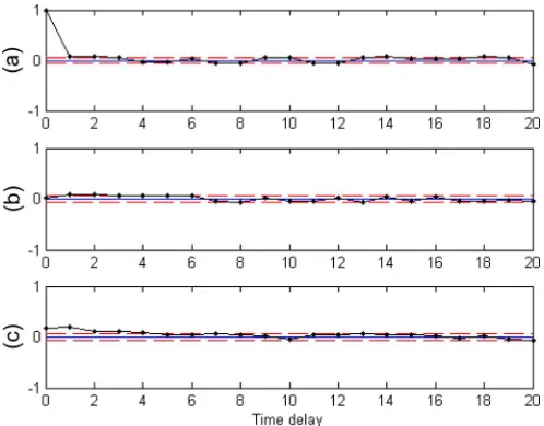
[image:5.594.303.551.321.517.2]Fig. 3. Validity tests for" in (25): (a) (); (b) (); and (c) ().
[image:6.594.304.553.65.260.2]Fig. 4. Validity tests for" in (25): (a) (); (b) (); and (c) ().
[image:6.594.41.289.302.498.2]Fig. 5. Validity tests for" in (25): (a) (); (b) (); and (c) ().
Fig. 6. Validity tests for" in (25): (a) (); (b) (); and (c) ().
so can be primarily considered as including omitted pre-dictable information in terms of delayed outputs. Fig. 6 clearly suggests that only lies outside the confidence interval that is correlated to the delayed outputs. It is clear that the three-guidelines-based analytic results are properly consistent with (25). The new guidelines can provide a useful indication of the insufficiencies of poor models.
Furthermore, consider the last two residuals that are all correlated to the delayed outputs. In Fig. 5, all the corre-lation functions significantly exceed the confidence limits,
particularly, and . It is because the variance of
(i.e., ) is much greater than the
variance of . Hence, the previous validity tests,
which only include and , can be used to
effec-tively detect the omitted term. Nevertheless, after decreasing
the parameter from to , both and display
very weak detection power since the variance of
(i.e., ) is much smaller than the variance of .
As shown in Fig. 6, only lies outside the confidence interval and detects correlated residual . It is evident that the new model validation method can provide an enhanced detection power.
Finally, table representations of the correlation function tests for (25) are presented in the Appendix to provide more numer-ical demonstrations.
IV. SIMULATIONSTUDIES
In this section, the new correlation test procedure is applied to two simulated examples to test the trained NNs in modeling of both nonlinear static function and nonlinear dynamical system.
Example 1: Using MLP to Approximate a Nonlinear Static Model
Consider a nonlinear discrete static model formulated as
[image:6.594.41.290.539.735.2]Fig. 7. Validity tests for network 1: (a) (); (b1) (); and (b2) ().
where and denote the noise-free output and measured noise contaminated output, respectively. The inputs and were set as uniformly distributed random data sequences with zero mean and amplitude from to . The noise was selected as a normally distributed random sequence with zero mean and variance of . Totally 500 data points were generated for each data sequence. In this study, MLP net-work with one hidden layer was used to identify the underlying model. Typically, MLP consists of a set of source neurons that constitutes the input layer, one or more hidden layer of com-putation neurons, and an output layer of comcom-putation neurons. Each layer was fully connected to the next layer and the input signal propagated through the network in a forward direction, on a layer-by-layer basis.
First, a 2-4-1 network (network 1) was determined to approx-imate the underlying model. The input vector and predicted output of network 1 are formulated as follows:
(27)
(28)
where denotes the number of the neurons in hidden layer, which is four. , , and denote the connection weight vector of output layer, connection weight, and bias vectors of hidden layer, respectively. is the activation functions of output layer and chosen linear combination. is the activa-tion funcactiva-tions of hidden layer and chosen tan-sigmoid funcactiva-tions. Levenberg–Marquardt algorithm [26] was used to train the net-work. After 5000 training epochs, the variance of the residuals converged to . Then, the validation procedure was used to check the quality of network 1. Since the underlying system
is static, has no significance but , , and
[image:7.594.304.550.325.514.2]were detected and displayed in Fig. 7.
Fig. 8. Validity tests for network 2: (a) (); (b1) (); and (b2) ().
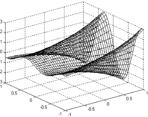
Fig. 9. Map ofz(t)versusu (t)andu (t)for (25).
As shown in Fig. 7, both and lie outside the
confidence interval at . Thus, the network is invalid. In other words, network 1 cannot comprehensively approximate the nonlinearity of the underlying system. To improve the quality of the identification, the number of neurons in the hidden layer was increased to ten (network 2). The inputs and predictive output were computed to be the same as in (27) and (28) with . After 2000 training epochs, the variance of residuals was reduced to , which is extremely close to the variance of the preset noise. Fig. 8 shows the results ob-tained from using the new validity tests that all the correlation functions lay inside the confidence interval that network 2 is valid.
[image:7.594.60.291.555.610.2]Fig. 10. Map of^z(t)versusu (t)andu (t)for network 1.
Fig. 11. Map of^z(t)versusu (t)andu (t)for network 2.
Figs. 9 and 10 suggest that the two maps are different so that network 1 did not capture all the characteristics of (25). In Fig. 11, the map for network 2 is nearly the same as the map of (25) in Fig. 9. Thus, network 2 can be used to properly ap-proximate the original model. It is clear that the results obtained from using the new validity tests are exactly in accord with the graphical analysis.
Example 2: Using NARX Network to Approximate Duffing Equation
In this study, the well-known Duffing [27] equation was se-lected to illustrate the validation of NN in approximating a com-plex nonlinear dynamic system. The most generally forced form of the Duffing equation is expressed as follows:
(29)
Fig. 12. Measured outputs and inputs for (30).
Subsequently, the Duffing equation was written as a system of first-order ordinary differential equations and the parameters were chosen as
(30)
where denotes an additive white noise such as measurement error and and denote the noise-free output and mea-sured output, respectively.
It should be noticed that for simulating continuous systems by computer, approximate solutions are obtainable by the applications of numerical methods, where a numerical solution is obtained at discrete values of the independent variable with a specified integration interval. To solve the ordinary differential equation, a number of numerical solutions, also named numer-ical integration, have been developed such as Euler’s method, Euler–Cauchy method, midpoint method, and fourth-order Runge–Kutta method. In this study, fourth-order Runge–Kutta algorithm with an integration interval of 3000 s was applied to simulate the response of the system to the input . The
initial values were set as , and . Equation
(30) on the interval of was investigated. A
sampling interval of 30 s was chosen and the resulting data sequences with length of 1500 were generated. Further details about the simulation method, integration interval, and sampling interval selections can be found from the studies of Aguirre and Billings [12], [28]. The noise was selected as a normally distributed data sequence with zero mean and
variance of . The measured inputs and outputs are
shown in Fig. 12.
[image:8.594.44.289.307.500.2]Fig. 13. NARX network.
selection method was used to select the lags of delayed inputs and outputs. The architecture of the network is shown in Fig. 13 [29].
The NN input selection for nonlinear system identification, which refers to the corresponding variable and lag (delay) se-lection, is to select significant regressors out of all the possible regressors. There are three main strategies for efficient input se-lection including forward sese-lection, backward elimination, and stepwise selection. In this study, forward selection associated with the new validity tests was applied to select the NN in-puts. First, regressors were added into the NN input set step by step. Then, the correlation tests were executed after each new input set was applied. While an NN was invalid, the three guide-lines were used as reference to assist in finding new significant regressors.
Initially, the lags of the inputs and outputs were selected as
, , and , respectively. The input set
and a 3-3-10-1 NARX network (network 3) were determined and expressed as shown in (31) and (32) at the bottom of the page, where denotes the length of the input vector which is three. , , and the training algorithm were determined to be the same as in Example 1. In addition, early stopping [29] was employed to avoid overfitting and improve the generalization of the network. The first 1000 pairs of data points were used to train the network. The inputs and the outputs with from 1001
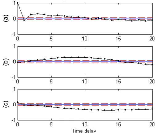
Fig. 14. Validity tests for network 3: (a) (); (b) (); and (c) ().
to 1500 were used as the validation set. After 22 training epochs, the variance of the residuals for the training set converged to and the variance of the residuals for the validation set converged to . Fig. 14 shows the validity tests for network 3.
As shown in Fig. 14, all correlation functions lie outside the confidence interval that network 3 is invalid. As discussed in Section III, whether and lie inside or outside, if lies outside the confidence interval, more regressors in terms of delayed outputs need to be initially superadded into to the network. To improve the quality of identification, the max-imum lag of the outputs was extended to 15. The corresponding 10-3-10-1 network (network 4) was determined with the same hidden layers and output layer as network 3 [(32) with ]. The input set for network 4 was assigned as
(33)
After 29 epochs, the variances of the training dada set residual and the validation data set residual were, respectively,
reduced to and . Compared to network 3, the
levels of the residuals were massively reduced. However, Fig. 15 shows the validity tests for network 4 that the network is still in-adequate and can be further improved since lies outside the confidence interval.
To improve the performance of the network, the maximum lag of delayed inputs was extended to 3. A 12-3-10-1 network
(31)
[image:9.594.62.268.65.310.2]Fig. 15. Validity tests for network 4: (a) (); (b) (); and (c) ().
Fig. 16. Validity tests for network 4: (a) (); (b) (); and (c) ().
(network 5) was determined and the corresponding input vector was assigned as
(34)
After 37 training epochs, and were, respectively,
re-duced to and . Compared to network 4, all
resid-uals have been obviously reduced. Fig. 16 shows that all corre-lation functions lie inside the confidence interval that network 5 is valid.
Discussion on the Validation Results: Two other sets of data sequences were also generated to comprehensively com-pare the performance of the three networks.
[image:10.594.39.556.301.514.2]Fig. 17. Noise-free outputs with different initial conditions.
Fig. 18. Measured outputs (output 3) and inputs (input 2).
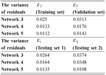
TABLE I
PERFORMANCECOMPARISON FOR THETHREENETWORKS
First, the underlying system displays exponentially sensitive dependence on initial conditions due to the chaotic behaviors of nonlinear dynamical systems [30]. To demonstrate the system under this condition, the initial values were slightly varied and
[image:10.594.340.517.561.686.2]TABLE II
VALIDATIONTESTS FORRESIDUAL" (t)
TABLE III
VALIDATIONTESTS FORRESIDUAL" (t)
TABLE IV
VALIDATIONTESTS FORRESIDUAL" (t)
TABLE V
VALIDATIONTESTS FORRESIDUAL" (t)
(testing set 1) was generated. Fig. 17 shows the noise-free out-puts with the different initial conditions. It is evident that the dif-ference between two outputs grows very rapidly with increasing time.
Second, the input signal of the system was replaced by a new signal as shown in Fig. 18. The measured outputs (testing set 2) of the system excited by the new inputs are also shown in Fig. 18. It is to be noticed that all the testing outputs are cor-rupted by new additive noise with the same level as in (30).
To compare the performance of the three networks under these conditions, the networks were applied to predict the measured outputs by using the new testing set. Table I shows
the variances of the residuals obtained from using the three networks that compared to the other two networks; network 5 provides a much better approximation to the underlying system. It is consistent with the correlation test results that only network 5 is adequate.
V. CONCLUSION
TABLE VI
VALIDATIONTESTS FORRESIDUAL" (t)
TABLE VII
VARIANCE OF THERESIDUALS ANDTERMS IN(25)
modeling and identification since it includes a direct com-bined ODCCF test between residuals and outputs. Compared to the previous approaches, it provides a more effective and comprehensive validity detection. In addition, based on the new validity tests, three guidelines have been also proposed in this study to provide some useful advise to tell why the NN is invalid and how to improve it. It has been shown through the simulation studies that the new methodology can be effectively used to validate static and dynamic NNs. As mentioned at the beginning of the study, it is hoped that this study could promote the awareness of why correlation tests should be used to validate identified neural networks and provide examples how to use the tests. Finally, with its generic applicability, the test procedure could be applied to validate other model sets such as classical linear and nonlinear models, wavelet models, fuzzy logic models, and so on.
APPENDIX
TABLE REPRESENTATION OF VALIDATIONRESULTS FOREXAMPLE(25)
Tables II–VI show the correlation test results for (25). As mentioned in Section III, if a correlation function is less than or around the confidence limits, the association between the two variables can be considered as uncorrelated or very weakly cor-related. In this study, the 95% confidence limits are computed
as . In Tables II–VI, bold face number
presents the correlation value, which is significantly greater than the confidence limits. As shown in the tables, the new correla-tion tests not only can detect the validity of the residuals, but also can indicate the insufficient of the residuals.
Table VII shows the variance of the residuals and terms in (25) that even though the variance of the omitted terms is much smaller than the variance of the residuals, the enhanced validity tests still can effectively detect the insufficiencies.
ACKNOWLEDGMENT
The authors would like to thank the editors and the anony-mous reviewers for their helpful comments and constructive suggestions during the revision of this paper.
REFERENCES
[1] D. Wedge, D. Ingram, D. McLean, C. Mingham, and Z. Bandar, “On global-local artificial neural networks for function approximation,” IEEE Trans. Neural Netw., vol. 17, no. 4, pp. 942–952, Jul. 2006. [2] M. Martinez-Ramon, J. L. Rojo-Alvarez, G. Camps-Valls, J.
Munoz-Mari, A. Navia-Vazquez, and E. Soria-Olivas, “Support vector ma-chines for nonlinear kernel ARMA system identification,”IEEE Trans. Neural Netw., vol. 17, no. 6, pp. 1617–1622, Nov. 2006.
[3] M. Liu, “Delayed standard neural network models for control systems,” IEEE Trans. Neural Netw., vol. 18, no. 5, pp. 1376–1391, Sep. 2007. [4] T. Hayakawa, W. M. Haddad, and N. Hovakimyan, “Neural network
adaptive control for a class of nonlinear uncertain dynamical systems with asymptotic stability guarantees,”IEEE Trans. Neural Netw., vol. 18, no. 5, pp. 80–89, Jan. 2007.
[5] L. Ljung, System Identification—Theory for the User, 2nd ed. Upper Saddle River, NJ: Prentice-Hall, 1999.
[6] T. Bohlin, “On the problem of ambiguities in maximum likelihood identification,”Automatica, vol. 7, pp. 199–200, 1971.
[7] T. Bohlin, “Maximum power validation of models without higher order fitting,”Automatica, vol. 14, pp. 173–146, 1978.
[8] G. E. P. Box and G. M. Jenkins, Time Series Analysis Forecasting and Control. San Francisco, CA: Holden-Day, 1976.
[9] T. Söderström and P. Stoica, “On covariance function tests used in system identification,”Automatica, vol. 26, pp. 125–133, 1990. [10] S. A. Billings and W. S. F. Voon, “Structure detection and model
va-lidity tests in the identification of nonlinear system,”Proc. Inst. Elec-tron. Eng., vol. 130, pt. D, pp. 193–199, 1983.
[11] S. A. Billings and W. S. F. Voon, “Correlation based model validity tests for nonlinear models,”Int. J. Control, vol. 44, pp. 235–244, 1986. [12] L. A. Aguirre and S. A. Billings, “Validating identified nonlinear models with chaotic dynamics,”Int. J. Bifurcat. Chaos, vol. 4, pp. 109–125, 1994.
[13] S. A. Billings and Q. M. Zhu, “Nonlinear model validation using cor-relation tests,”Int. J. Control, vol. 60, pp. 1107–1120, 1994. [14] S. A. Billings and Q. M. Zhu, “Model validation tests for multivariable
nonlinear models including neural networks,”Int. J. Control, vol. 62, pp. 749–766, 1995.
[15] Q. M. Zhu and S. A. Billings, “Properties of higher order correlation function tests for nonlinear model validation,” inProc. 23rd Int. Conf. Ind. Electron. Control Instrum., New Orleans, LA, 1997, vol. 1, pp. 306–310.
[16] K. Z. Mao and S. A. Billings, “Multi-directional model validity tests for non-linear system identification,”Int. J. Control, vol. 73, pp. 132–143, 2000.
[17] L. F. Zhang, Q. M. Zhu, and A. Longden, “A set of novel correlation tests for nonlinear system variables,”Int. J. Syst. Sci., vol. 38, no. 1, pp. 47–60, 2007.
[19] I. J. Leontaritis and S. A. Billings, “Input-output parametric models for nonlinear systems, part 1 and part 2,”Int. J. Control, vol. 41, 1985, pp. 303–328, 329–344.
[20] S. Chen and S. A. Billings, “Representation of nonlinear systems: The NARMAX,”Int. J. Control, vol. 49, pp. 1012–1032, 1989.
[21] , G. W. Irwin, K. Warwick, and K. J. Hunt, Eds., Neural Network Appli-cations in Control. London, U.K.: Institution of Electrical Engineers, 1995.
[22] L. A. Aguirre, “A nonlinear correlation function for selecting the delay time in dynamical reconstructions,”Phys. Lett. A, vol. 203, pp. 88–94, 1995.
[23] L. A. Aguirre, “On the structure of nonlinear polynomial models: Higher order correlation functions, spectra, and term clusters,”IEEE Trans. Circuits Syst. I, Fundam. Theory Appl., vol. 44, no. 5, pp. 450–453, May 1997.
[24] H. Hjalmarsson, “Asymptotic correction tests in model validation,” inProc. 32nd Conf. Decision Control, San Antonio, TX, 1993, pp. 2058–2059.
[25] A. H. Bowker and G. J. Lieberman, Engineering Statistics. Engle-wood Cliffs, NJ: Prentice-Hall, 1972.
[26] M. T. Hagan and M. Menhaj, “Training feedforward networks with the Marquardt algorithm,”IEEE Trans. Neural Netw., vol. 5, no. 6, pp. 989–993, Nov. 1994.
[27] A. H. Nayfeh and D. T. Mook, Nonlinear Oscillations. New York: Wiley, 1979.
[28] L. A. Aguirre and S. A. Billings, “Digital simulation and discrete mod-eling of chaotic system,”J. Syst. Eng., vol. 4, pp. 195–215, 1994. [29] S. Haykin, Neural Networks: A Comprehensive Function. Upper
Saddle River, NJ: Prentice-Hall, 1999.
[30] P. G. Drazin, Nonlinear Systems. Cambridge, U.K.: Cambridge Univ. Press, 1992.
Li Feng Zhangreceived the B.Sc. degree in elec-tronic engineering from Heilongjiang University, Harbin, China, in 1999, the M.Sc. degree in radio frequency and communication engineering from the University of Bradford, Bradford, U.K., in 2003, and the Ph.D. degree from the Faculty of Computing, Engineering and Mathematical Sciences (CEMS), University of the West of England (UWE), Bristol, U.K., in 2007.
Currently, he is a Lecturer at the Department of Economic Information Management, School of In-formation, Renmin University of China, Beijing, China. His research interests lie in the following fields: nonlinear dynamic system identification, mathemat-ical modeling (e.g., NARMAX model), intelligence modeling [artificial neural networks (ANN) and fuzzy inference systems (FIS)], model validation, variable selection, and model structure selection.
Quan Min Zhu received the Ph.D. degree from Faculty of Engineering, University of Warwick, Warwick, U.K., in 1989.
Currently, he is the Professor in Control Systems at the Faculty of Computing, Engineering and Math-ematical Sciences (CEMS), University of the West of England (UWE), Bristol, U.K. His main research interest is in the area of nonlinear system modeling, identification, and control. Recently, he started inves-tigating electrodynamics of acupuncture points and sensory stimulation effects in human body, modeling of human meridian systems, and building up electro-acupuncture instruments. He has published over 100 papers on these topics.
Prof. Zhu is an Associate Editor of theInternational Journal of Systems Sci-enceand an editor of theInternational Journal of Modeling, Identification and Control.
Ashley Longdenreceived the B.Sc. degree in elec-trical and electronic engineering from University of Bath, Bath, U.K., in 1971.