The First Stage Studies of U-State Space Control System Design
LIU Xin
1, ZHU Quanmin
1, NARAYAN Pritesh
1, YANG Ye
21. Department of Engineering Design and Mathematics, University of the West of England, Frenchay Campus, Coldharbour Lane, Bristol, BS16 1QY, UK
E-mail: [email protected], [email protected], [email protected]
2. Beijing Aerospace Automatic Control Institute, Beijing, China E-mail: [email protected],
Abstract: In this study, a basic idea of U-state feedback control system design method is proposed based on U-model principle. Compared with U-model based nonlinear polynomial systems, the U-state space design is to determine the desired state variable equation x td( ), therefore to find the controller output u t( 1) . The desired state equation can be designed/specified and transformed into the U-state space expression easily. The controller output can be obtained from resolving the equation. The desired state variables are updated by the corresponding state variables x t( ). Assume that the state variables are measurable or obtained by a proper observer in this study. In case studies, two nonlinear discrete time state space models are selected to test the proposed approach. Computational experiments, that is, simulation studies, are used to demonstrate the procedure effectiveness.
Key Words: U-model framework, U-control approach, U-state space framework, feedback linearization
1
Introduction
State space model based linear control system design approaches have been well studied in research and adopted in wide range of applications. In linear case, the polynomial models can be easily converted into state space model by standard realization approaches. However a nonlinear polynomial model is very difficult to convert it into state space expression. The most popular method of nonlinear state space control system design is feedback linearization [1, 2] (input-state linearization and input-output linearization), which is to convert the nonlinear state space model into linear expression. The central idea of feedback linearization is to convert the non-linear model into a linear form by coordinate transform, so as to cancel the non-linear dynamics in the closed-loop [3]. Then use linear state space approaches to design the corresponding control systems. However this is a case by case approach with certain degree of skills in manipulating different equations and selecting coordinates.
In regarding to nonlinear polynomial models, there is a generic systematic approach, which is called U-model approach, to convert nonlinear polynomial model into a controller output u t( 1) based time-varying polynomial model. The U-model covers almost all existing smooth nonlinear discrete time polynomial models as its subsets. This original U-model polynomial expression was first proposed in [4]. In progression along this route, the first time of the U-model was named in a study of pole placement controller design for nonlinear plants [5]. A summary of the first decade research development has been reported [6]. Although various linear controller design approaches such as predictive control, adaptive control and sliding model control have been developed and demonstrated for nonlinear
* This work is partially supported by Department of Engineering Design
and Mathematics, University of the West of England under PG travel grant, the National Nature Science Foundation of China under Grant 61273188, and Taishan Scholar Funding, Shandong, China
models within U-model framework, the emphasis has been put on nonlinear polynomial models. In regarding to using linear state space design approaches for nonlinear polynomial models, there has been a recent research proposing a U-block model [3] defined as a general input output model, which is formulated by a revised U-model based pole placement control system from polynomial models. Then linear equivalent U-state space model can be realised. The U-block model bridges between the linear state space control system design and nonlinear polynomial models.
The U-state space model framework has been explained in [7], which is converted state equation and output equation into a prototype model with respect of controller output
( 1)
u t and the corresponding time-varying state variables. However the model properties and control design methods have not been developed. The related analysis and ideas on the model expression, mapping and operations need to be studied and discussed.
2
U-model based control system design
2.1 U-model
Consider a general nonlinear polynomial plant model below.
0
( )
( (
1) ,..., (
), (
1) ,..., (
))
( )
( )
y u
L
l l l
y t
f y t
y t n
u t
u t n
y t
p t
(2.1) where y t( )R and u t( )R are the output and input (also known as controller output in control system design) of the plant respectively at discrete time instant t(1, 2, …), the regression terms
p t
l( )
are the products of past inputs and outputs such as u t( 1) ( y t3), u t( 1) ( u t2), y t2( 1),and
l are the associated parameters. Typically, forexample, linear time invariant difference equation based plant models and NARMA (nonlinear auto-regressive moving average) models [8].
U-model is defined as, under a U mapping from the above polynomial model, a controller output u t( 1) oriented polynomial below,
2
( ) ( (*), U( 1))
(*) ( ( 1) ,..., ( ), ( 2) ,..., ( ), )
U( 1) ( 1) ( 1) M( 1)
y t f t
y t y t n u t u t n
t const u t u t u t
(2.2)
The corresponding U-model is defined as below
0
( )
M( ) (
j1)
j j
y t
t u t
(2.3)This is expanded from the above nonlinear function f(.) as a polynomial with respect to u t( 1) . where M is the degree of model input (controller output) , the time varying
parameter vector
10
( ) ( ) ( ) M
M
t t t R
is afunction of past inputs, outputs (u(t-2), …, u(t-n), y(t-1), …,
y(t-n)), and the parameters
(
0
L)
in (2.1).Such an example, from polynomial model to the U-model conversion, is shown below.
The polynomial model is [11]
2
( ) 0.1 ( 1) ( 2)
0.5 ( 1) ( 1) 0.8 ( 1) ( 2)
y t y t y t
y t u t u t u t
(2.4)
And the U-model can be determined in notation of (2.3)
2
0 1 2
( ) ( ) ( ) ( 1) ( ) ( 1)
y t t t u t t u t (2.5)
where 0( ) 0.1 ( 1) (t y t y t2), 1( ) 0.8 (t u t2), and 2( )t 0.5 ( 1)y t
.
2.2 U-control system design
In order to use linear polynomial mode based design approaches, define the desired plant output as y td( ), which is specified either by designers or customers in advance. Accordingly the relationship between a specified plant output y td( ) and the requested corresponding controller output u t( 1) can be expressed in terms of U-model
0
( ) M ( ) (j 1)
d j
j
y t t u t
(2.6)Accordingly this establishes a prototype for proposing a new two-step design procedure [3].
Step 1(design y td( )): The first task of the design is to determine the desired plant output y td( ) according to a specified performance index, for example, pole placement control (PPC) [5]
( ) ( ) ( ) d
Ry t Tw t Sy t (2.7)
where y t( ) , y td( ) and w t( ) are the plant output, desired/designed plant output, and reference input respectively. The polynomials R, S, and T are used to specify the desired plant output y td( ).
Step 2 (workout u t( 1) ): Then the remaining design task is to resolve one of the roots of (2.7) to obtain the controller output u t( 1) . That is
1
0
( 1) ( ) M ( ) (j 1) 0
d j
j
u t y t t u t
(2.8)where 1
is a root-solving algorithm, such asNewton-Raphson algorithm [13]. A detailed analysis on the root solving issues has been presented [14]. The block diagram of U-model based pole placement control system is shown in figure 2.
) 1 (t
Fig. 1: U-model based pole placement control system
2.3 U-block model
As mentioned in previous section, the U-block model is converted from nonlinear polynomial through U-model expression (2.3) and then assigned with required poles through a linear feedback controller design. The function of U-block model can be expressed as
( ) d( ) ( ) ( )
c
T T
y t y t w t w t
R S A
(2.9)
where w t( ) is the reference input, y t( ) is system output, ( )
d
y t is desired plant output and R S, and T are the polynomial of the forward shift operator. The polynomial
c
A is the closed loop characteristic equation. Figure 1 shows the U-block model structure
Fig. 2: U-block model
3
U-state space Control system design
3.1 Design with U-state space models
Consider a nonlinear discrete time state space system ( 1) ( ( ), ( ))
( ) ( ( )) x t f x t u t y t h x t
(3.1)
where x t( )Rn, u t( )R, y t( )R are the state variable, system input and output respectively. ( , ) n l
f R R is a n-dimensional smooth vector field.
In order to use linear state feedback design approaches, define the desired state variable as x td( ).
( 1) ( ) ( )
d d d
x t A x t B w t (3.2)
Accordingly the task of the design is to determine the desired state variable x td( ) according to specified performance index A Bd, d.
With reference to U-model (2.3), in simple mathematical expression, it is clear to express (3.2) as
0
( ) M ( ) (j 1)
dn j
j
x t t u t
(3.3)where j( )t contains the state variable x t( ).
Consider a desired closed loop state space model [4]
1
d d d
d d
x t A x t B w t y t C x t D w t
(3.4)
where A B C Dd, d, d, d is the state description matrices desired closed loop system. Ad is determined by the closed loop characteristic equation. Cd is determined by the closed loop zeroes. The state equation is expressed as
1 1
2 2
1 1
( 1) ( 2) 1
0 1 0 0
( 1) ( ) 0
0 0 1 0
( 1) ( ) 0
0 0 1
( 1) ( ) 0
( 1) ( ) 1
k k
dk d k d k d
k k
x t x t
x t x t
w t
x t x t
a a a a
x t x t
(3.5)
The output equation is expressed as
1 2
1 2 1
1 ( ) ( ) ( ) , , , , ( ) ( ) ( )
dk dk d d
n n
x t x t
y t dw t
x t x t (3.6)
The corresponding transfer function of (3.4) is
1 2 1 2 1 1 ... ( ) ... n n
d d dn
n n
d dn
z z
g z d
z a z a
(3.7)
where the closed loop characteristic equation is determined by the denominator of (3.7).
Assume that the state variable x t( ) are measurable or obtained by a proper observer, the desired state space equation can be updated from (3.2).
As mentioned in section 2.2, the remaining design task is to resolve one of the roots of (3.3) to obtain the controller output. That is
1( ( ), )
d y t Nonlinear plant ( (u t 1), )
y(t) ( 1)
u t
( ) d y t T R S R
-
U-control systemw(t) y(t)
1
0
( 1) ( ) M ( ) ( 1) 0j
d j
j
u t x t
t u t
(3.8)where 1
* is a root-solving algorithm, such asNewton-Raphson algorithm. A detailed analysis on the root solving issues has been presented [15].
For the U-state space design approach, the desired plant output x td( ) is obtained by closed loop state equation (3.2), and then controller output u t( 1) equation can be converted from the state equation x t( ) (3.3). To resolve the criterion function (3.2) to determine the designed/desired state variable x td( 1). Then obtain the controller output
( 1)
u t through equation (3.8), that is, resolve one of the roots from the equation (3.8). With this procedure, it only uses the state space equation, in U-state space expression, to obtain controller output u t( 1) in the first stage. The system output can be obtained by the state equation. For a nonlinear state space model, the calculation is merely to resolve one of the roots from the U-state space (3.3).
Especially, it has the following root solver for a linear desired state space equation (3.8)
0 1
( ) ( ) ( 1)
( ) dn
x t t
u t
t
(3.9)
3.2 State observer for nonlinear model
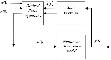
In this study, assume all the state variables are measurable. Otherwise proper observers must be designed, which will be presented in the future publications. The desired block diagram of the U-state space control system with a proper observer is show in the figure 3.
Fig. 3: Block diagram of U-state space control system
3.3 The proposed state feedback control system design procedure
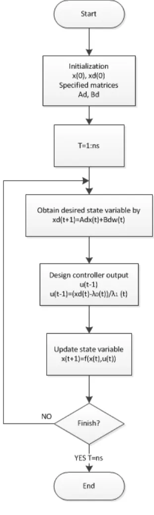
Without losing generality, assume all state variables are measurable or could be obtained by the proper state observer. Accordingly a step-by-step procedure for the U-state space control system design for state space models can be specified as following:
Step 1. Setup the initial state variables value (0), (0)
d
x x . Specify the dynamic matrix Ad, input matrix Bd of the desired state equation.
Step 2. To predict the next step desired state variable ( 1)
d
x t , substitute the corresponding specified matrices and state variables x t( ) (3.2).
Step 3. Obtain controller output u t( 1) from (3.8). Step 4. Update state variable x t( ) from (3.1)
Step 5. Go back to Step 2 until the end of the simulation time.
Figure 4 shows the flow chart of the Matlab program implementation.
Desired State equations
State observer
Nonlinear state space model
y(t) u(t)
x(0)
t xˆ [image:4.595.65.301.562.691.2]Fig. 4: Matlab program flow chart
4
Case studies
In case study, two nonlinear discrete time state space models are selected to test the proposed methodology. The same closed loop specifications are assigned for these models to demonstrate that the proposed method is generally suitable for controlling different dynamics. Assume that the state variables are measurable or obtained by a proper observer.
The desired closed loop characteristic equation is specified with
2 0.2 0.3
c
A q q (4.1)
Therefore the closed loop poles are a complex conjugate pair of 0.1 0.5385 i , which gives equivalently in continuous time domain of damping ratio 0.3980 and undamped natural frequency 1.5100 rad/s. To achieve zero steady state error, specify
0 c(1) 1 0.2 0.3 1.1
w A (4.2)
According to (3.5) and (3.6), the specified closed loop standard controllable realisation of (4.1) is
0 1 0
1.1 0 0
0.3 0.2 1
d d d d
A B C D
(4.3)
It can be found that
2( 1) ( ( ), ( ), ( ))1 2
d
x t f x t x t u t (4.4)
Therefore the controller output u(t) can be determined by solving the equation (3.9).
Case I: Consider a nonlinear discrete time state space system [13]
2
1 1 2
2 2 1
1
( 1) ( ) ( ) ( 1) ( ) cos ( ) ( ) ( ) ( )
x t x t x t
x t x t x t u t y t x t
(4.5)
where x ii, 1, 2 are state variables, and u t( ), y t( )are control input and system output.
From system (4.5), the desired state equation xd2( )t can
be expressed as
2( 1) 0( ) 1( ) ( 1)
d
x t t t u t (4.6)
where 0( )t x t2( 1)cos ( 1) x t1 , 1( ) 1t .
From (4.6), the controller output is determined by
2 0
1
( 1) ( ) ( 1)
( ) d
x t t
u t
t
(4.7)
Set up the initial state variables
1(0) 0.5, (0)2 0.5
x x , and the desired state variables
1(0) 0, 2(0) 0
d d
Fig. 5: Response of state variable x t1( )
Fig. 6: Response of state variable x t2( )
Fig. 7: Controller output u t( )
It can be inspected from Figures 5-7 that the state variable
1( )
x t reaches the peak value at 5s with overshoot 0.12. After 13s, the responseofstatevariable x t1( ) settles down. Compared with x t1( ), the state variable x t2( ) has a lower
overshoot but similar oscillation. Within the first 8s, the controller output fluctuates between 0.04 to -0.1, and it settles down at about 13s. The results of the controller output show an appropriate amplitude level and tuning profile.
Case II: Consider the following nonlinear discrete time
model [1]
1 1 2 1
2 2 2 1 1
1
( 1) ( ) ( ) sin ( )
( 1) (t) ( ) cos ( ) cos 2 x ( ) ( ) ( ) ( )
x t x t x t x t
x t x x t x t t u t
y t x t
(4.8)
where x t( ) is state variable, and u t( ), y t( )are control input and system output.
From (4.8), the desired state equation xd2( )t can be
expressed as
2( 1) 0( ) 1( ) ( 1)
d
x t t t u t (4.9)
where 0( )t x t2( )x t2( )cos ( )x t1 , 1( ) cos 2 ( )t x t1 .
The controller output is determined by solve equation (4.9). The same initial specification in previous case is used in simulation. The simulation results are shown in the following figures 8-10.
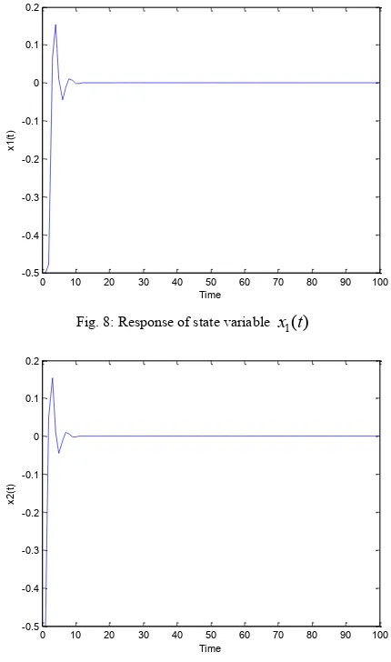
Fig. 8: Response of state variable x t1( )
Fig. 9: Response of state variable x t2( )
0 10 20 30 40 50 60 70 80 90 100 -0.5
-0.4 -0.3 -0.2 -0.1 0 0.1 0.2
Time
x1
(t
)
0 10 20 30 40 50 60 70 80 90 100 -0.5
-0.4 -0.3 -0.2 -0.1 0 0.1 0.2
Time
x2
(t
)
0 10 20 30 40 50 60 70 80 90 100 -0.12
-0.1 -0.08 -0.06 -0.04 -0.02 0 0.02 0.04
Time
C
on
tr
ol
le
r
ou
tp
ut
u
(t
) -0.50 10 20 30 40 50 60 70 80 90 100
-0.4 -0.3 -0.2 -0.1 0 0.1 0.2
Time
x1
(t
)
0 10 20 30 40 50 60 70 80 90 100 -0.5
-0.4 -0.3 -0.2 -0.1 0 0.1 0.2
Time
x2
(t
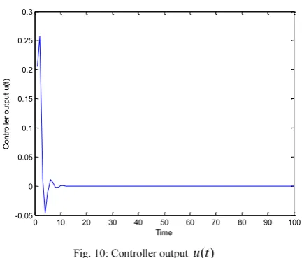
[image:6.595.56.272.367.619.2]Fig. 10: Controller output u t( )
It can be inspected from Figures 8-10 that the state variable x t1( ) reaches the peak value at 4s with overshoot
0.16. After 15s, the responseofstate variable x t1( ) settles down. Compared with x t1( ), the state variable x t2( ) has a
similar oscillation.
The simulation results give a strong indication that the proposed U-state space approach could be applied to design most practical industrial systems (subject to certain level of nonlinearity) initially, even though a lot of bench tests will be conducted in the following thorough validation work.
5
Conclusions
This work has established a platform for using linear state space approach to design nonlinear state space models. Initial simulation studies have indicated the feasibility of the procedure to be expanded to the design of nonlinear robust control system in a straightforward routine.
References
[1] Slotine, J.E. and Li, W., Applied nonlinear control, Prentice Hall, London, 1991.
[2] Isidori, A., Nonlinear control systems (3rd ed.), Berlin: Springer-Verlag, 1995.
[3] Zhu, Q.M., Zhao, D.Y. and Zhang, J.H., A general U-block model based design procedure for nonlinear polynomial control systems, 2014 (have been accepted).
[4] Zhu, Q.M., Identification and Control of nonlinear systems, PhD thesis, University of warwick, UK, 1989.
[5] Zhu, Q.M. and Guo, L.Z., A pole placement controller for nonlinear dynamic plants, Journal of Systems and Control Engineering, Proceedings of the Institution of Mechanical Engineers Part I, 216(6): 467-476, 2002.
[6] Xu, F.X., Zhu, Q.M., Zhao, D.Y., and Li, S.Y., U-model based design methods for nonlinear control systems–A survey of the development in the 1st decade, Control and Decision, 28(7): 961-971, 2013 (in Chinese).
[7] Zhu, Q.M., Li, S.Y. and Zhao, D.Y., A universal U-model based control system design. In Proceedings of the 33rd Chinese Control Conference, July 28-30, Nanjing China, 28-30 July 2014: 1839-1844.
[8] Billings, S.A., Nonlinear System Identification: NARMAX Methods in the Time, Frequency, and Spatio-Temporal Domains, Wiley, John & Sons, Chichester, West Sussex, 2013.
[9] Chong, E.K.P. and Zak , S.H., An Introduction to Optimization, (4th ed.), Wiley, Purdue University, 2013. [10] Ogata, K., Modern Control Engineering (5th ed.),
Prentice-Hall, 2009.
[11] Du, W.X., Wu, X.L, and Zhu, Q.M., Direct design of U-model based generalized predictive controller (UMGPC) for a class of nonlinear (polynomial) dynamic plants, Proc. Instn. Mech. Enger, Part I: Journal of Systems and Control Engineering, 226: 27-42, 2012.
[12] Dorf, R.C. and Bishop, R.H., Modern control systems (8th ed), Addison-Wesley, 1998.
[13] Xiang, Z.R., Cheng, Q.W. and Hu, W.L., Feedback control of nonlinear discrete-time systems based on observers, Control Theory and Applications, 18(1): 80-82,2001 (in Chinese). [14] Zhu, Q.M., Wang, Y.J,, Zhao, D.Y., Li, S.Y., and Billings,
S.A., Review of rational (total) nonlinear dynamic system modelling, identification and control, Int. J. of Systems Science, 2014 (in press).
[15] Liu, X., Peng, Y., Zhu, Q.M., and Narayan, P. and Xu, F.X., U-model based LMI robust controller design.In Proceedings of the 33rd Chinese Control Conference, July 28-30, Nanjing China, 28-30 July 2014: 2200-2205.
[16] Astrom, K.J. and Wittenmark, B., Adaptive control (2nd ed).
Reading: Dover, 1995.
0 10 20 30 40 50 60 70 80 90 100 -0.05
0 0.05 0.1 0.15 0.2 0.25 0.3
Time
C
on
tr
ol
le
r
ou
tp
ut
u
(t