Original citation:
Halac, Marina and Prat, Andrea. (2016) Managerial attention and worker performance. American Economic Review.https://www.aeaweb.org/journals/aer
Permanent WRAP URL:
http://wrap.warwick.ac.uk/81644
Copyright and reuse:
The Warwick Research Archive Portal (WRAP) makes this work by researchers of the University of Warwick available open access under the following conditions. Copyright © and all moral rights to the version of the paper presented here belong to the individual author(s) and/or other copyright owners. To the extent reasonable and practicable the material made available in WRAP has been checked for eligibility before being made available.
Copies of full items can be used for personal research or study, educational, or not-for-profit purposes without prior permission or charge. Provided that the authors, title and full
bibliographic details are credited, a hyperlink and/or URL is given for the original metadata page and the content is not changed in any way.
Publisher’s statement:
Permission to make digital or hard copies of part or all of American Economic Association publications for personal or classroom use is granted without fee provided that copies are not distributed for profit or direct commercial advantage and that copies show this notice on the first page or initial screen of a display along with the full citation, including the name of the author. Copyrights for components of this work owned by others than AEA must be honored. Abstracting with credit is permitted.
A note on versions:
The version presented here may differ from the published version or, version of record, if you wish to cite this item you are advised to consult the publisher’s version. Please see the ‘permanent WRAP URL’ above for details on accessing the published version and note that access may require a subscription.
Managerial Attention and Worker Performance
∗
Marina Halac
†Andrea Prat
‡May 5, 2016
Abstract
We present a novel theory of the employment relationship. A manager can
invest in attention technology to recognize good worker performance. The
technology may break and is costly to replace. We show that as time passes
without recognition, the worker’s belief about the manager’s technology
worsens and his effort declines. The manager responds by investing, but
this investment is insufficient to stop the decline in effort and eventually
becomes decreasing. The relationship therefore continues deteriorating,
and a return to high performance becomes increasingly unlikely. These
deteriorating dynamics do not arise when recognition is of bad performance
or independent of effort.
∗An earlier version of this paper was circulated under the title “Managerial Attention and
Worker Engagement.” We thank Dirk Bergemann, Simon Board, Patrick Bolton, Alessandro Bonatti, Sylvain Chassang, Wouter Dessein, Marco Di Maggio, Bob Gibbons, Ricard Gil, Chris Harris, Ben Hermalin, Johannes H¨orner, Navin Kartik, Amit Khandelwal, Qingmin Liu, Michael Magill, Jim Malcomson, David Martimort, Niko Matouschek, Meg Meyer, Daniel Rap-poport, Paolo Siconolfi, Matt Stephenson, Steve Tadelis, various seminar and conference audi-ences, and four anonymous referees and the Co-editor for helpful comments. Enrico Zanardo and Weijie Zhong provided excellent research assistance.
What motivates employees to work hard? A large literature in economics
has been devoted to this question, focusing for the most part on the optimal
design of (explicit or implicit) incentive contracts and on how workers respond to different forms of compensation.1 In this paper, we provide a novel theory of
the employment relationship: workers’ effort depends not only on compensation,
but also on their beliefs about whether management is paying attention to their
behavior. Only when paying attention can management recognize (good or bad)
worker behavior. Because attention is costly and not directly observable, the
moral hazard problem that arises inside the firm is two-sided: workers must be
incentivized to exert effort; managers must be incentivized to invest in attention.
The idea that workers care about whether they are being “watched” is related
to the widely studied Hawthorne effect, namely the improvement in workers’ per-formance possibly caused by the “feeling that they are being accorded some
at-tention” (Oxford English Dictionary). Interpretations of the original Hawthorne
experiments and why workers’ behavior may change with their awareness of being
observed vary.2 Our focus is on workers who care about managerial attention
be-cause this attention can produce some form of recognition of their performance.
Workers value recognition for either psychological or financial reasons, or both.
More broadly, our theory is in line with the psychology literature that examines
the determinants of worker productivity. This literature finds that employee job
satisfaction and workers’ perceptions about management matter for both produc-tivity and profits (Judge et al. 2001; Ostroff 1992; Harter, Schmidt and Hayes
2002). In particular, whether workers believe that they are given “recognition
or praise for doing good work” affects their engagement and performance (
Har-ter et al., 2002, p. 269), and these beliefs can have a significant impact on an
organization’s bottom line (Harter et al.,2010).3
We model managerial attention as a technology that recognizes worker
per-formance. For example, consider a chief operating officer (COO) and a division
1For an excellent survey, seePrendergast (1999).
2The Hawthorne effect originated in a set of experiments conducted in a Western Electric factory in the 1920s, where workers’ productivity was shown to increase each time a change in lighting was made. For a recent reassessment, seeLevitt and List(2011).
head or director in a firm. These parties meet regularly to discuss how the
di-rector is handling business, yet the relevant cost of monitoring for the COO is
not attending the meetings but rather learning and thinking about the tradeoffs, challenges, constraints, and opportunities in the director’s division. The acquired
understanding allows the COO to recognize good ideas and decisions by the
di-rector for some time. Eventually, however, the COO’s attention is needed in
other areas and she may lose grasp of the division’s issues—something the
direc-tor cannot directly observe. We capture these ideas by introducing an attention
technology, an intangible asset that is subject to depreciation and in which a
manager can invest. At any point in time, the manager can recognize a worker’s
performance only if she has a high attention technology in place.4
Can managers be induced to invest in attention technology? How is workers’ effort affected by their perceptions of managerial attention? We provide a model
where these two variables are interlinked and explore their dynamic interaction.
We show that relationship dynamics depend on the monitoring structure. When
recognition is of good performance, dynamics are deteriorating: absent
recogni-tion, worker effort and eventually managerial investment decrease, and a return
to high productivity becomes less likely over time. These dynamics contrast with
those that arise when recognition is ofbad performance or independent of effort.
Our model is cast in continuous time. At each moment, a myopic agent
privately chooses effort which generates output for a principal. Output is unob-servable; instead, the parties observe a verifiable signal—“recognition”—whose
instantaneous arrival rate depends on the principal’s attention technology and
the agent’s effort. If the principal’s technology is high, the arrival rate is
propor-tional to effort; if the technology is low, recognition cannot arrive. Recognition
yields the agent a fixed reward, which may be purely psychological or also
en-tail a monetary bonus. The principal’s attention technology follows a stochastic
process akin to those used for productive assets in the industrial organization
lit-erature (e.g., Besanko and Doraszelski,2004): a high technology can “break” at
4Another illustrative example of managerial attention is in continuous process improvement, pioneered by Toyota and imitated by scores of manufacturing firms (Gibbons and Henderson,
any point and become low, and the principal can invest at some cost to instantly
“fix” it. The agent observes neither the principal’s investment nor her
atten-tion technology, which we thus call the principal’s type. Naturally, the agent’s incentive to exert effort depends on his belief that the principal’s type is high.
There are several important features of managerial attention that our model
tries to capture. First, workers cannot perfectly assess the quality of the
atten-tion technology. A manager’s ability to identify and document the contribuatten-tions
made by workers depends on many different and interrelated aspects of
manage-ment, which are themselves difficult to observe.5 Second, the signals produced by
the attention technology are (at least in part) verifiable, typically because they
describe the details of contributions made by workers in a specific context
famil-iar to them. As the COO in the example above, a manager cannot learn those details unless a high technology is in place; hence, she cannot simply “fake”
recognition at random times. Third, as noted, attention is an asset, although
our analysis imposes no restrictions on how likely the technology is to break at
any point.6 Lastly, unlike with productive assets, the manager does not care
about the attention technology directly; attention is valuable only insofar as it
incentivizes the agent to exert effort.
We focus on continuous equilibria, where the agent’s belief about the
prin-cipal’s type is continuous in the absence of observable events. This belief is a
function of recognition (or lack thereof) and the agent’s belief about the princi-pal’s investment. Because recognition reveals that the principrinci-pal’s type is high,
the belief jumps up to one when the agent is recognized. Without investment,
the agent’s belief, and thus his effort, would then decrease continuously as time
passes without recognition, due to Bayesian updating and the possibility that
the attention technology breaks down. But a principal whose technology breaks
could invest to fix it, with certainty or with a high probability, and if the agent
5One reason for this is that management practices display synergies with other practices and attributes of the firm, as stressed byMilgrom and Roberts(1990,1995),Ichniowski, Shaw and Prennushi(1997),Bartling, Fehr and Schmidt(2012), andBrynjolfsson and Milgrom(2013).
expected that to be the case, his belief about the principal’s type would stop
de-creasing. We show however that this does not occur in equilibrium: the principal
invests in attention technology as the agent’s belief declines, but this investment is insufficient and in fact becomes decreasing when the agent gets pessimistic
enough. Relationship dynamics as a result feature continuous deterioration:
ab-sent recognition, effort and eventually investment go down, and the chances of
obtaining recognition and reverting to high performance decline.
We contrast the dynamics of this model in which the principal can recognize
good performance with those that arise when she can also recognize bad
perfor-mance. Suppose that if a high attention technology is in place, a verifiable bad
signal arrives at a rate that is decreasing in the agent’s effort. The agent incurs a
(psychological or monetary) penalty when a bad signal arrives. We show that if recognition is primarily of bad performance, or symmetric and thus independent
of effort, the model is essentially static: the agent’s belief and effort, as well as
the principal’s investment, remain constant absent recognition once the principal
starts investing. The relationship therefore does not fall into deterioration.
Our results show that the presence in an organization of the two-sided moral
hazard problem we study has important implications for the dynamics of the
employment relationship. When a manager must invest in attention to recognize
a worker’s behavior, the worker’s belief about attention affects both his incentives
to work and the manager’s incentives to invest, with non-obvious consequences that depend on how recognition relates to worker effort. Our findings illuminate
a distinction that had not been identified: the literature on firm reputation
(reviewed below) assumes that learning is exogenous, hiding the implications of
different forms of endogenous learning.
Related literature. This paper fits into the literature on firm reputation; see
Cripps(2006) andBar-Isaac and Tadelis(2008) for surveys. Most closely related
are Board and Meyer-ter-Vehn (2013,2014) and Dilm´e(2014), where a firm can
invest in product quality and consumers learn about quality through Poisson
signals.7 We apply the theory of reputation to study dynamics inside the firm:
rather than analyzing how a firm’s reputation for quality affects sales, we
ex-amine how a firm’s reputation for attention affects worker productivity. More
importantly, we depart from the literature by endogenizing the learning process: whereas in these models of firm reputation consumers observe exogenous signals
of firm quality, in our model the rate at which information arrives depends on
the agent’s action. Marinovic, Skrzypacz and Varas(2015) study firm reputation
when information is endogenously generated by the firm via voluntary
certifi-cation. We instead focus on the dynamics generated by the complementarity
between the principal’s and agent’s actions.8
Our work is also related to an extensive literature on monitoring, which
stud-ies the problem of monitoring or auditing an agent when the monitor cannot
commit to a strategy. Early contributions such asGraetz, Reinganum and Wilde
(1986), Khalil(1997), and Strausz(1997) analyze static settings. More recently,
Dilm´e and Garrett (2014) study a dynamic model where in each period an
in-spector can either wait or inspect a short-lived potential offender, incurring a
cost for changing her action. While our focus is on recognition of good behavior,
monitoring in this literature is of bad behavior, as in the case that we study in
Section 3.
Often motivated by the persistent performance differences across seemingly
similar firms thatGibbons and Henderson(2013) document, a series of recent
pa-pers emphasize path dependence in equilibrium dynamics. For example,
Callan-der and Matouschek (2014) study a search model in which managers learn about
the quality of managerial practices by trial and error, and show that if practices
are complementary, quality is persistent over time. Chassang (2010) finds that
efficient equilibria can be path dependent in a repeated game in which a party
learns to predict her partner’s cost of cooperating over time. Li and Matouschek
(2012) show that bad shocks can have persistent effects in a relational contracts
model in which a principal’s cost of making payments to an agent is privately
observed. Our paper is related in that it also generates persistent relationship
about the principal’s type in our model; we distinguish between good and bad signals about the (uninformed) agent’s performance.
8Unlike in our model, moral hazard is only one-sided inBoard and Meyer-ter-Vehn (2013,
2014), Dilm´e (2014), and Marinovic et al. (2015). This is also the case in Ely and V¨alim¨aki
dynamics. Unlike these articles, however, we consider a model of reputation, in
which workers’ beliefs about management’s attention play a central role.
Finally, by studying managerial attention, our paper relates to Geanakop-los and Milgrom (1991) and other work on organizations under cognitive limits,
although we address different issues.9 This literature is concerned with the
coor-dination of agents without conflicting interests, while we consider how an
atten-tion technology interacts with incentive provision.10 The role of attention is also
stressed in empirical work on the time use of managers and firm productivity,
including Bandiera et al. (2011) and Bandiera, Prat and Sadun (2013).
1
The model
Setup. Consider a principal and an agent. Time t ∈ [0,∞) is continuous
and infinite. At each time t, the agent privately chooses effort at ∈ [0,1] at
instantaneous cost c(at) = 12a2t. The principal receives an output flow equal to
at. This output however is unobservable; instead, the parties observe a verifiable
signal which we call recognition.
Recognition arrives via a (non-homogeneous) Poisson process with parameter
µθtat, where µ > 0 and θt ∈ {L, H} is the state of the principal’s attention
technology at time t, with L= 0 and H = 1. The agent receives a reward b >0 each time he is recognized. For most of our analysis, we take this reward to be
a purely psychological benefit, so it is exogenously fixed and entails no costs for
the principal. This is in line with our motivation and allows us to focus on the
problem of attention costs rather than the problem that the principal may want
to save on agent compensation. Section 4considers the case in which the reward
is a monetary bonus chosen and paid by the principal.
The evolution of θt is determined by an exogenous Poisson process and
en-dogenous investment. Specifically, at any time t, a high attention technology
becomes low (“the technology breaks”) with instantaneous probability γ > 0,
9SeeGaricano and Prat(2013) for a survey of this literature.
and the principal can invest at any point by paying a lump sum cost F > 0 to
instantly transform a low technology into a high one (“fix the technology”).11
The simple form of depreciation is assumed for tractability. The assumption that the principal can instantly fix the technology is not only convenient but also
appealing: it removes additional frictions and thus yields a simple benchmark
for our model, as we show below.
The agent observes neither the principal’s investment nor her attention
tech-nology, which we thus call the principal’s type.
A “heuristic timing” of the game within each instant is as follows: first, the
principal decides whether to fix the technology (if low) and the agent chooses
ef-fort; next, recognition arrives or not and the agent receives a reward accordingly;
finally, the attention technology (if high) breaks or not.
A remark on terminology: the principal’s attention technology is a
“monitor-ing technology.” However, “monitor“monitor-ing” is typically used in the literature (see our
review in the Introduction) as referring to monitoring that is of bad rather than
good performance, and a flow rather than an asset. We use the term “attention”
to make clear the distinction with our assumptions.
Strategies and payoffs. Let hAt− be the agent’s private history up to (but
not including) time t, consisting of the history of effort choices and recognition
(public signal) arrival times up tot. A (pure) strategy for the agent specifies, for
each hAt−, a choice of effort at t, at. This strategy, a= {at}t≥0, is progressively measurable with respect to the filtration induced by the histories hAt−. The principal’s private history is denoted hP t− and consists of the history of type
realizations (equivalently, θ0, investment decisions, and depreciation shocks) and
recognition arrival times up to t. A strategy for the principal specifies, for each
time t at which the technology breaks (i.e. the type switches from high to low)
11We model attention as a capital asset in dynamic industrial organization models. In
and history up to time t, hP t−, a cumulative distribution Q(z, t) over the time
z ≥ t to invest in fixing it. This strategy, Q = {Q(z, t)}z≥t,t≥0, is progressively measurable with respect to the filtration induced by the historieshP t−. Note that the investment plan chosen by the principal at any timetat which the technology
breaks will be sequentially optimal. In particular, since nothing happens until
the principal invests—as the type remains low in the absence of investment and
no recognition can occur while the type is low—the principal will want to follow
the prescribed distribution.
The agent’s belief that the principal’s type is high at (the beginning of) time
t is xt ≡ EQ,xe 0[θt|hAt−] ∈ [0,1], where Qe = {Qe(z, t)}z≥t,t≥0 is the agent’s belief about the principal’s investment strategy and x0 ∈ (0,1] is the exogenous and
commonly known prior belief.12 That is, the agent’s belief about the principal’s type depends on the history of effort and recognition arrival times through the
conjectured investment strategy Qe and prior x0. Since xt is then a function of
hAt− only and we assume the agent’s effort strategy to be progressively
measur-able, x={xt}t≥0 is also progressively measurable.
Both parties are risk neutral. For tractability and to focus on the dynamic
incentives of the principal, we assume that the agent is myopic;Section 4
consid-ers the case of a forward-looking agent. Given belief xt and effortat, the agent’s
(instantaneous) expected payoff at time t≥0 is
Ut=µxtatb−
1 2a
2
t.
The first-order condition for the optimal choice of effort, given belief xt, is
at=µxtb. (1)
To rule out corner solutions, we assume:
Assumption 1. µb≤1.
Hence, condition (1) always pins down the agent’s optimal level of effort.
12
e
Qcould be a non-trivial probability distribution overQ. In this case,Qeis a Borel
The principal discounts future payoffs at rate r > 0. Denote by (Tj)∞j=1 the (stochastic) instants at which the principal’s attention technology breaks. Let
P(z, Tj, Tj+1)≡ Q(QT(z,Tj)
j+1,Tj) be the cumulative distribution over the time to invest
in fixing the technology that the principal chooses at time Tj given that the
technology breaks again at Tj+1, which implies that the principal must have invested in between these times (only a high technology can break). Then given
a={at}t≥0 andQ={Q(z, t)}z≥t,t≥0, the principal’s expected payoff at time 0 is
π0 =EQ,θ0
"
Z ∞
0
e−rtatdt−
∞
X
j=1
Z Tj+1
Tj
e−rzF dP(z, Tj, Tj+1)
#
.
Equilibrium. Each time there is recognition, the agent learns that the
prin-cipal’s type is high, so his belief is reset to xt = 1. The agent receives no
information about the principal’s type until recognition again occurs. We there-fore restrict attention to equilibria in strategies that depend only on what has
happened since the last recognition (see, e.g.,Board and Meyer-ter-Vehn,2014).
With a slight abuse of notation, we drop the time index in our analysis and write
all variables as a function of the time that has passed since recognition, denoted
by s.
Analogous to the definitions above, a strategy for the agent is a = {as}s≥0 (progressively measurable with respect to the filtration induced by the
histo-ries hAs−) and a strategy for the principal is Q={Q(z, s)}z≥s,s≥0 (progressively measurable with respect to the filtration induced by the histories hP s−). An equilibrium is a quadruple (a, Q,Q, xe ) such that: (i) given x, a maximizes the
agent’s (instantaneous) expected payoff; (ii) givena,Qmaximizes the principal’s
expected payoff; (iii) Qeis correct; and (iv) given aandQe,xis updated by Bayes’
rule. Acontinuous equilibrium is an equilibrium in which xsis continuous for all
s ≥0.13 That is, in a continuous equilibrium, the agent’s belief as a function of
time t is continuous in the absence of publicly observable events. In any
contin-uous equilibrium,Q(z, s) must be continuous, and we will further assume in this
case that it is absolutely continuous, so it admits a density function. We then
take the principal’s strategy in a continuous equilibrium to simply specify an
instantaneous probability of investment as a function of the time since
recogni-tion and the principal’s current type (note that past type realizarecogni-tions are payoff irrelevant for the principal given her current type). More precisely, in a
contin-uous equilibrium, the principal’s strategy specifies an instantaneous investment
probability qs for each time s ≥ 0 conditional on a low type at s, θs = L (and
zero investment if θs =H). The agent’s belief about qs is denoted qes.
Observable attention benchmark. Before turning to the equilibrium
analy-sis, consider a benchmark in which the principal’s attention technology is
observ-able by the agent. It follows from (1) that the agent’s effort at any time t ≥ 0
is at = µb if θt = H and at = 0 if θt = L. Take now any time t at which the
technology breaks. For any δ >0, the principal prefers to fix the technology at
time tand then again at t+δ if it breaks by then, rather than waiting and fixing
the technology at time t+δ, if and only if
Z δ
0
e−(γ+r)τµbdτ −F − 1−e−γδ
e−rδF ≥ −e−rδF.
Integrating and simplifying this expression yields that the principal fixes her
at-tention technology whenever it breaks if and only ifµb≥(γ+r)F, that is, if and
only if the resulting increase in output is larger than the instantaneous rental
cost of capital, given by the risk of breakdown plus the interest rate. It is imme-diate that this condition is also necessary for the principal to invest in attention
technology when the technology is unobservable by the agent. Throughout our
analysis, we thus assume that parameters are such that this condition is satisfied:
Assumption 2. µb≥(γ+r)F.
2
Relationship dynamics
Unlike in the observable attention benchmark described above, in equilibrium the principal cannot fix her attention technology each time it breaks when attention is
type is high isxs = 1 at alls ≥0, but then the agent always exerts effortas =µb
and the principal has no incentives to invest at cost F.
We construct a continuous equilibrium in which the principal does not invest if the time that has passed since recognition iss < s, for an endogenous threshold
time s∈(0,∞), and she mixes between investing and not investing ifs ≥s. We
show that any continuous equilibrium with positive investment must take this
form, and one such equilibrium exists if the cost of investmentF is small enough.
Consider first the agent’s belief about the principal’s type, xs. At s = 0 this
belief is x0 = 1, since recognition fully reveals that the type is high. Then, given
no recognition, the change in xs is given by three sources: (i) the possibility
that a high attention technology breaks, with instantaneous probability γ; (ii)
learning about the technology in the absence of recognition, according to Bayes’ rule; and (iii) the agent’s belief about the principal’s investment, which must be
correct in equilibrium (i.e. qes=qs). If qs is continuous on a given open interval,
then locally in that interval the evolution of xs is governed by
˙
xs=−γxs−xs(1−xs)µas+ (1−xs)qs. (2)
This law of motion is similar to that in Board and Meyer-ter-Vehn (2013), with an important difference: our Bayesian learning term, xs(1−xs)µas, depends on
the agent’s action as, while it is only a function of xs in their paper (see their
equation 2.2). In our setting the learning process is endogenous and depends
on the agent’s behavior; as shown in Section 3, this difference has important
implications for the dynamics of the relationship.
In the equilibrium we are constructing, the principal does not invest before the
threshold time s is reached. Hence, for s < s, the law of motion for xs becomes
˙
xs=−γxs−xs2(1−xs)µ2b, (3)
where we have substituted as = µxsb. Solving this differential equation with
initial condition x0 = 1 uniquely pins down the agent’s belief and effort ats < s.
Naturally, xs and as are strictly decreasing over this time period: since the
high as time passes without recognition, both because of Bayesian updating and
because the probability that the principal’s technology has broken goes up.
Consider next the principal’s incentives to invest. Let πHs be the principal’s expected payoff at s when her type is θs =H and πLs when her type is θs = L.
The principal is willing to invest atsonly ifπL
s ≤πHs −F. Since, by construction,
at any point in this equilibrium the principal either does not want to invest or
is indifferent between investing and not, πL
s ≥πHs −F for all s ≥ 0 and we can
write the expected payoffs for the two principal types as
πLs =
Z ∞
s
e−r(τ−s)aτdτ , (4)
πHs =
Z ∞
s
e−(γ+r)(τ−s)−Rsτµazdz a
τ +γπLτ +µaτπH0
dτ . (5)
The low type’s expected payoff at any point is simply the output given by
the agent’s effort. To interpret the high type’s expected payoff, note that the
instantaneous probability that her technology breaks at any time is γ, and the
instantaneous probability that recognition occurs given a high type at time z is
µaz. Thus, between times s and τ, the probability that no breakdown occurs is
e−γ(τ−s), and the probability that no recognition occurs, given no breakdown, is
e−Rsτµazdz. So long as neither breakdown nor recognition occurs, the high type
receives the output flow. If the technology breaks at time τ, her continuation
payoff is πLτ, whereas if recognition occurs, her continuation payoff is πH0 .
To convey the economic intuitions more clearly, let Ψs ≡ πH0 − πHs denote
the principal’s value of recognition at time s and Λs ≡ πHs −πLs her value of
investing at s. At each time s ≥ s in the equilibrium, the principal follows a
mixed strategy, so she must be indifferent between investing and not investing:
Λs=F. (6)
It follows that ˙Λs = 0 for alls ≥s, which combined with (4)-(6) yields
Ψsµas= (γ+r)F. (7)
s, given by the value of recognition times the instantaneous probability of
recog-nition conditional on a high type. Equation (7) says that, for the principal to be
indifferent at each time s ≥ s, her instantaneous benefit of investment must be equal to the instantaneous rental cost of capital at all such times. The
instanta-neous benefit of investment must therefore be constant for s ≥s, which implies
that the agent’s effort must be decreasing (increasing) at any such time at which
the value of recognition is increasing (decreasing). Our main result shows that
the value of recognition is in fact strictly increasing, and hence effort strictly
decreasing, at all times s ≥ s in the equilibrium; moreover, effort becomes low
enough that the principal’s investment must become strictly decreasing as well.
Proposition 1. Fix any set of parameters (γ, µ, b, r). There exist F > 0 and
F ∈ (0, F) such that a continuous equilibrium with positive investment exists if and only if the cost of investment is F ≤ F, and all continuous equilibria have
positive investment if F ≤F. In any continuous equilibrium with positive
invest-ment, the principal does not invest if the time that has passed since recognition
is s < s, for a threshold time s ∈ (0,∞); at s ≥ s, the principal invests with a
continuous instantaneous probability qs ∈ (0,∞) which is strictly decreasing for
s > s large enough. The agent’s belief xs and effort as, and thus the
uncondi-tional instantaneous probability of recognition µxsas, are continuous and strictly
decreasing for all s ≥ 0. If r ≤ γ, the value of s, and thus the continuous
equilibrium with positive investment, are unique.
Proof. See Appendix A. Q.E.D.
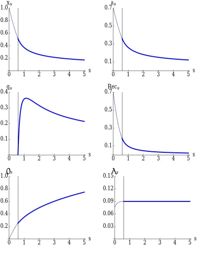
Figure 1illustrates the equilibrium. When the agent’s belief is relatively high,
the principal’s benefit from being revealed to be a high-attention type is small. Following recognition, there is thus a period of time during which the principal
does not invest. As time passes and the agent’s belief and effort go down, the
principal’s value of recognition increases, until at time s the principal finds it
optimal to start investing. The principal’s investment however is insufficient to
stop the decline in effort, and at some point it also begins to decline. Hence,
as time goes by without recognition, both the agent’s effort and the principal’s
0 1 2 3 4 5 s 0.2
0.4 0.6 0.8 1.0xs
0 1 2 3 4 5 s
0.1 0.3 0.5 0.7as
0 1 2 3 4 5 s
0.1 0.2 0.3 0.4qs
0 1 2 3 4 5 s
0.1 0.3 0.5 0.7Recs
0 1 2 3 4 5 s
0.2 0.4 0.6 0.8 1.0Ys
0 1 2 3 4 5 s
[image:16.612.112.500.122.617.2]0.03 0.06 0.09 0.12 0.15Ls
Figure 1: Equilibrium dynamics. Parameters are γ = 1, F = 0.09, µ = 1,
b = 0.7, and r = 0.01. Recs is the unconditional instantaneous probability of
As mentioned, the intuition for why the agent’s effort decreases prior to s
is immediate. But why must effort continue going down at s ≥ s while the
principal invests? Recall from (7) that the principal’s indifference condition yields Ψs = (γ+µars)F. Moreover, by definition, ˙Ψs = ˙Λs − π˙Ls, and thus for s ≥ s,
˙
Ψs =−π˙Ls =as−rπLs; that is, the value of recognition increases (decreases) ats
if current effort is above (below) the long-run future average. We can then show
that ˙Ψsand ˙ascannot change signs at a times > s. For a stark intuition, suppose
effort were decreasing up to s0 and increasing from then on, for s0 > s. Then both the value of recognition Ψs and the conditional probability of recognition
µas would be lower at s0 than right before this time. But since the principal
is indifferent at s0, she would have strict incentives to invest right before, a contradiction. Hence, effort as must be a monotonic function over s≥s, and in
fact an analogous argument shows that it cannot be a strictly increasing function.
It follows that the agent’s effort is either constant or strictly decreasing for
all s ≥ s. We prove that it must indeed be strictly decreasing in equilibrium
by showing that not only the agent’s belief is continuous but also the change in
the belief must be continuous. Specifically, the equilibrium must satisfy smooth
pasting: ˙xs is continuous at s. Since ˙xs <0 for s < s, this implies that ˙xs, and
thus ˙as, are strictly negative in a right neighborhood of s, and therefore for all
s ≥s. The logic for smooth pasting is similar to that above, namely it is needed
to provide the principal the right amount of incentives to invest at each point. Suppose for the purpose of contradiction that ˙xs and thus ˙as were to jump at
s. Clearly, they can only jump up (recall qs = 0 at s < s), and since ˙Ψs is
continuous,14 the change in the principal’s instantaneous benefit of investment,
µ Ψ˙sas+Ψsa˙s
, would then also jump up ats. However, sinceµ Ψ˙sas+Ψsa˙s
= 0
froms on by condition (7), this would implyµ Ψ˙sas+ Ψsa˙s
<0 for s < s close
enough to s, and therefore (using (7) again) Ψsµas > (γ +r)F for such times.
The contradiction is then immediate: the principal would have strict incentives
to invest in attention technology before reaching the threshold time s.15
14Note that ˙Ψ
s= ˙Λs−π˙Ls, where ˙π L
s =−as+rπLs and ˙Λs= (γ+r)Λs−µasΨsare continuous. 15More formally: observe that, as noted infn. 14, ˙Λ
A principal who delays investment is therefore punished with continuous
dete-rioration of the relationship. The agent becomes more pessimistic and his effort
declines over time, so that even if the principal then decides to invest, it is harder to obtain recognition and return to high performance. In fact, we can show that
in the limit for an infinitely patient principal, the equilibrium gives rise to a
trap as the moral hazard problem becomes more severe. Consider the limit as
the discount rate r goes to zero and let the principal’s cost of investment be
F < F so that the equilibrium of Proposition 1 exists. Appendix B shows that
as F approaches F, lims→∞xs and lims→∞as vanish: the probability of
obtain-ing recognition and revertobtain-ing to high performance goes to zero as time passes
without recognition.16
Proposition 1also shows that the equilibrium investment path is hump-shaped. The logic is elaborate because the principal uses a mixed strategy, but to see the
main idea, take the aforementioned case in which the agent’s belief and effort
go to zero absent recognition. At one extreme, it is clear that the principal will
not invest when the agent’s belief is close to one, as the value of recognition
is then close to zero. At the other extreme, it is also clear that as the agent’s
belief approaches zero, the principal’s investment must go to zero: as shown
by (2), if xs = 0, ˙xs is determined by (the agent’s correct belief over) qs, so
xs, and hence as, would increase in equilibrium if qs > 0. More generally, we
show that punishing the principal for not investing requires effort to become low enough over time that investment must eventually become decreasing for effort
to continue declining.
Finally, about uniqueness: two arguments are used to show that any
contin-uous equilibrium with positive investment must be as characterized in
Proposi-tion 1. First, we show that any such equilibrium where, at each time s ≥ 0,
the principal either is indifferent or does not have incentives to invest, must take
this form. Second, we show that a continuous equilibrium where the principal
has strict incentives to invest over some time interval does not exist. Intuitively,
in any such equilibrium, the principal should strictly want to invest at s = 0;
otherwise, if she has strict incentives to invest at s0 >0 but not before, xs must
either increase continuously toward one as s approaches s0 or jump to one at s0, neither of which can occur. However, since Ψ0 = 0, the principal will not want to invest at s = 0. As for the result that any continuous equilibrium must be as
described in Proposition 1 ifF is small enough, this follows from the fact that a
no-investment equilibrium does not exist in that case: without investment, effort
decreases as time passes without recognition, but then for F sufficiently small
the principal eventually has strict incentives to invest to obtain recognition.17
3
Recognition of good and bad performance
We have considered a principal who can recognizegood performance by the agent.
What happens if she can also recognize bad performance? Recognition is more
likely to be of good performance in jobs based on innovation, where the verifiable
event is the presence of something positive like a breakthrough. Recognition of
bad performance, on the other hand, may arise in jobs where employees perform
well-defined tasks, like maintenance or quality control, and the verifiable event
is the presence of something negative like a fault.
Take the model of Section 1 but assume now that there are two types of
(verifiable) signals: good-performance signals and bad-performance signals. A good signal arrives via a Poisson process with parameter µθtat, whereas a bad
signal arrives via a Poisson process with parameter νθt(1−at), where µ, ν ≥0.
The agent receives a rewardb >0 when a good signal arrives and incurs a penalty
b < 0 when a bad signal arrives. Analogous to (1) and Assumption 1, for any
t ≥0, the agent’s effort isat=xt(µb−νb), where we assume µb−νb≤1.
The benchmark case where the principal’s attention technology is observable
is qualitatively the same as that inSection 1. In this setting with good- and
bad-performance signals, the principal invests in attention if and only if µb−νb ≥
(γ+r)F; analogous to Assumption 2, we assume that this condition holds.
Now suppose that the principal’s attention technology is unobservable by the
agent. Each time recognition—of either good or bad performance—occurs, the
agent learns that the principal’s type is high and thus his belief is reset to one.
As in Section 2, we consider equilibria in strategies that depend only on what has happened since recognition last occurred. Let s be the time since
recogni-tion. We characterize a continuous equilibrium (i.e., an equilibrium in which the
agent’s beliefxs is continuous) in which the principal does not invest in attention
technology if s <bs, for an endogenous threshold time bs∈(0,∞), and she mixes
between investing and not if s ≥sb.
Consider the law of motion for the agent’s belief xs. At s = 0, the belief
is x0 = 1. Then, given no recognition, the evolution of the belief on any open
interval over which qs is continuous is governed by
˙
xs =−γxs−xs(1−xs)[µas+ν(1−as)] + (1−xs)qs. (8)
Before timebsis reached, the principal does not invest. Substitutingas =xs(µb−
νb) andqs = 0 into (8), the law of motion for s <bs is
˙
xs =−γxs−xs(1−xs)[(µ−ν)xs(µb−νb) +ν]. (9)
Solving this differential equation with initial condition x0 = 1 pins down the
agent’s belief and effort at s <bs.
Consider nows ≥bs. The principal must be indifferent between investing and
not investing at these times. Analogous to (7), indifference yields
Ψs[µas+ν(1−as)] = (γ+r)F. (10)
Condition (10) shows that the sign of µ−ν is key in determining the qualitative
properties of the solution. If µ−ν > 0, the solution is qualitatively the same
as that in Section 2. Suppose instead that µ−ν ≤ 0. Then (10) shows that
the agent’s effort as and the principal’s value of recognition Ψs must move in
the same direction for the principal’s instantaneous benefit of investment to be
constant for s ≥ bs. Now since ˙Ψs = as−rπLs, it follows that effort must be
strictly increasing (decreasing) at any time s ≥ bs at which it is strictly above
from the long-run average at any such time. Therefore, when µ−ν ≤0, as and
Ψs must be constant for s ≥bs.
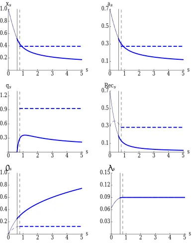
Proposition 2. Consider a setting with recognition of good and bad performance.
If recognition is primarily of good performance (i.e. µ > ν), the continuous
equi-libria are as characterized in Proposition 1. Suppose instead that recognition is
primarily of bad performance or symmetric (i.e. µ ≤ ν). Then in any
continu-ous equilibrium with positive investment, the principal does not invest if the time
that has passed since recognition is s < bs, for a threshold time bs ∈ (0,∞), and
she invests with a constant instantaneous probability qb∈ (0,∞) for s ≥ bs. The
agent’s belief xs and effort as are decreasing for s < bs and constant for s ≥ bs.
The unconditional instantaneous probability of recognition, xs[µas +ν(1−as)],
is constant for s≥bs.
Proof. See Appendix C. Q.E.D.
Figure 2 illustrates the equilibria. When recognition is primarily of bad
per-formance or symmetric, the equilibrium is essentially static: the principal’s in-vestment is zero initially and constant after it jumps up at the threshold time
b
s; the agent’s belief and effort and the unconditional instantaneous probability
of recognition are also constant for s ≥ bs.18 Hence, unlike when recognition is
primarily of good performance, the relationship does not continue deteriorating
over time.
The intuition for these results stems from the principal’s incentives to invest
in attention technology. The principal’s instantaneous benefit of investment is
the product of the instantaneous probability of recognition conditional on a high
attention technology and the value of recognition. When recognition is of bad performance or symmetric, a decline in the agent’s effort has a direct effect of
(weakly) increasing the principal’s incentive to invest because it (weakly)
in-creases the probability of obtaining recognition. However, when recognition is of
good performance, a decline in effort has a negative direct effect, as the
probabil-ity of recognition goes down. Consequently, incentivizing the principal to invest
0 1 2 3 4 5 s 0.2
0.4 0.6 0.8 1.0xs
0 1 2 3 4 5 s
0.1 0.3 0.5 0.7as
0 1 2 3 4 5 s
0.3 0.6 0.9 1.2 qs
0 1 2 3 4 5 s
0.1 0.3 0.5 0.7Recs
0 1 2 3 4 5 s
0.2 0.4 0.6 0.8 1.0Ys
0 1 2 3 4 5 s
[image:22.612.113.501.99.587.2]0.03 0.06 0.09 0.12 0.15Ls
Figure 2: Equilibrium dynamics when recognition is of good performance (solid lines) and when recognition is of bad performance (dashed lines). We set µ= 1 and ν = 0 in the former case and µ = 0 and ν = 1 in the latter; all other parameters are the same as in Figure 1. Recs is the unconditional instantaneous
probability of recognition, given byxs[µas+ν(1−as)]. The vertical lines indicate
in this case requires that her value of recognition increase; that is, she must be
threatened with continuously decreasing effort over time.
Our results have implications for the study of firm reputation. Note that when recognition is symmetric (µ = ν), the instantaneous probability with which a
signal arrives is independent of the agent’s effort. This case corresponds to
the one typically studied in models of firm reputation. For example, Board
and Meyer-ter-Vehn(2013) consider a setting in which consumers observe public
signals of the quality of a firm’s product, but the arrival rate of these signals
is independent of consumers’ actions (which are not explicitly modeled). The
reputational dynamics they obtain are as we characterize for the case ofµ≤ν.19
In reality, however, consumers are more likely to learn about the quality of
a product when the volume of sales is larger, both because more consumers experience with the product directly and because more consumers are likely to
learn from the experience of others.20 To map our model into this problem,
take θs to be firm quality, xs consumers’ expectation of firm quality, and as
the volume of sales at time s. The case studied in Board and Meyer-ter-Vehn
(2013) is one in which the firm sells a single unit at each time and consumers
compete in a Bertrand fashion, so the product price equals xs and as is fixed.
But another possibility is for the price to be fixed and quantity to adjust, so that
the volume of salesasis an increasing function of perceived qualityxs, analogous
to our model in Section 2. Here sales will change with perceived quality and in turn affect the rate at which information about quality is generated. As shown
in Proposition 1 and Proposition 2, this effect leads to qualitatively different
reputational dynamics.
4
Discussion
Forward-looking agent. For tractability and to focus on the principal’s
dy-namic incentives, we assumed throughout that the agent is myopic. The presence
of a forward-looking player and a myopic one is in line with the literature on firm
19Specifically, see the case of a convergent cutoff in their perfect good news setting.
reputation. In practice, however, workers are not fully myopic, and they can
ben-efit from experimenting: unlike a myopic agent, they value having information
in the future about whether managerial attention is high or low.
While we cannot solve the model with a forward-looking agent analytically, we
can numerically construct an equilibrium analogous to the one in Proposition 1
and show that it yields qualitatively the same relationship dynamics as with a
myopic agent. Consider the setting of Section 1, in which recognition is of good
performance, but assume now that the agent is forward-looking and discounts
the future at the same rate r >0 as the principal. The agent’s expected payoff
following recognition is
U0 =
Z ∞
0
e−R0s(r+µxτaτ)dτ
µxsas(b+U0)− 1 2a
2
s
ds.
For intuition, note that the instantaneous probability assigned by the agent to
recognition occurring at a time τ is µxτaτ, and hence his belief that recognition
will not occur by time s is e−R0sµxτaτdτ. When recognition occurs, the agent
receives the reward b plus an expected continuation payoff U0.
The agent chooses an effort plan {as}s≥0 to maximize U0 subject to the law of motion for xs given in equation (2), where qs is taken as given. Appendix D
sets up the Hamiltonian for the agent’s problem and derives the first-order con-ditions.21 We then solve for a continuous equilibrium that parallels the one we
constructed in Section 2: for a threshold time s ∈ (0,∞), the principal does
not invest if the time that has passed since recognition is s < s and she mixes
between investing and not investing if s≥s.
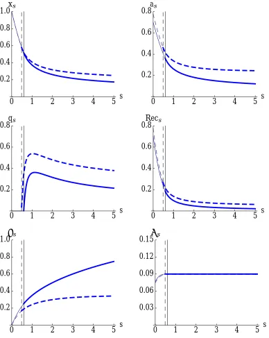
Figure 3 provides a graphical illustration. The figure shows that the
equilib-rium dynamics are qualitatively the same with a forward-looking agent and with
a myopic agent. As expected, though, there are quantitative differences. We
find that in the forward-looking agent case, the agent’s effort and the principal’s
investment are higher. The intuition is related to the value of experimentation
mentioned above: because a forward-looking agent benefits from knowing in the
0 1 2 3 4 5 s 0.2
0.4 0.6 0.8 1.0xs
0 1 2 3 4 5 s
0.2 0.4 0.6 0.8as
0 1 2 3 4 5 s
0.2 0.4 0.6 0.8qs
0 1 2 3 4 5 s
0.2 0.4 0.6 0.8Recs
0 1 2 3 4 5 s
0.2 0.4 0.6 0.8 1.0Ys
0 1 2 3 4 5 s
[image:25.612.113.501.114.601.2]0.03 0.06 0.09 0.12 0.15Ls
Figure 3: Equilibrium dynamics with a myopic agent (solid lines) and with a forward-looking agent (dashed lines). Parameters are the same as in Fig-ure 1. Recs is the unconditional instantaneous probability of recognition, given
future whether the principal’s type is high or low, for any given belief about
the principal’s current type, his incentive to exert effort is higher than that of
a myopic agent. Given the complementarity between effort and investment, the principal in turn invests more when the agent is forward-looking.
Recognition reward. In our model, the recognition reward b entails no costs
to the principal and has a fixed exogenous value. This formulation is appealing if
the reward is taken to be purely psychological. Suppose we instead take b to be
(partly) a monetary bonus. Then our model has assumed that this bonus is paid
not by the principal but by some external, unmodeled party, and that its value is
set exogenously. The first assumption is convenient to focus on the moral hazard
problem due to the principal’s cost of investment and abstract from another source of moral hazard: if the principal incurs the cost of the bonus directly, she
may want to decrease her investment in attention technology to save on this cost.
The second assumption is a natural consequence of the first.
Our qualitative results are unchanged if we remove the first assumption while
keeping the second one. That is, suppose b is an exogenously set bonus but
the principal bears the cost of bonus payments. We can incorporate this by
simply re-defining the principal’s payoff following recognition asπH0 ≡πH0 −b; our analysis can then be performed without change. The dynamics of the relationship
are qualitatively the same as in our main model; quantitatively, of course, the
principal’s incentives to invest will now be lower.
Allowing for an endogenous (and time-varying) bonus, on the other hand, can
lead to different dynamics, as the principal may increase the bonus over time
to boost the agent’s incentives. While a full solution to this case is beyond the
scope of this paper, we highlight here a negative result: endogenizing the bonus
does not eliminate the inefficiency in effort. To see why, suppose by contradiction
that the agent’s effort is always at the efficient level. Then the principal does not
invest, as she receives the largest possible payoff when her attention technology
is low and she bears no investment nor bonus costs. It follows that in
equilib-rium the agent’s belief about the principal’s type must go down as time passes without recognition,22 and inducing efficient effort requires the bonus to become
arbitrarily high over time. However, the high type is not willing to offer such a
high bonus: the gain is no larger than the present value of future efficient effort,
while the cost is proportional to the bonus as the high type has to pay the agent if recognition occurs before her technology breaks.
5
Conclusion
This paper has studied a dynamic two-sided moral hazard problem in which a
worker chooses effort and the manager chooses whether to invest in an attention
technology to recognize worker performance. We showed that when recognition is
of good performance, the relationship falls into deterioration: absent recognition, worker effort and eventually managerial investment decrease, and a return to high
productivity becomes less likely as time passes. These deteriorating dynamics do
not arise when recognition is of bad performance or independent of effort.
Our work highlights the role of workers’ beliefs about managerial attention.
These beliefs have important implications for the dynamics of the employment
relationship, particularly in jobs such as those based on innovation, where workers
are rewarded for good contributions rather than punished for bad outcomes.
We find that, as workers get pessimistic about the presence of a monitoring
system that can recognize their contributions, they reduce their effort, and even if management then improves its monitoring system, it will find it difficult to
restore its reputation. More broadly, our paper contributes to the theory of
reputation by endogenizing the learning process and uncovering the effects of
different forms of endogenous learning.
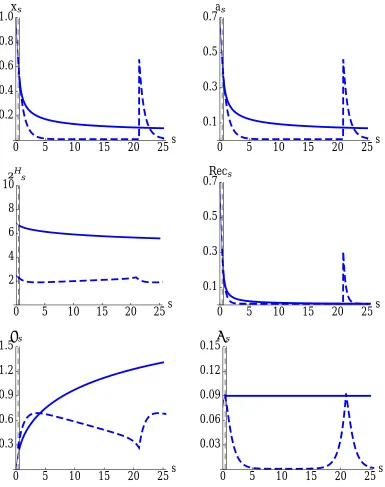
Our analysis restricted attention to continuous equilibria. There also exist
discontinuous equilibria of our game, in which the worker’s belief jumps in the
absence of recognition. Discontinuous equilibria can in principle take many
arbi-trary forms. In Appendix E, we study a simple class of stationary discontinuous
equilibria: as a function of the time since recognition, the manager invests only in
countably many points, where the time in between these points is fixed and the manager invests with the same mass probability at each of them. We show that
the manager prefers a continuous equilibrium, as characterized in Proposition 1,
to any discontinuous equilibrium in this class. A characterization of the whole
set of equilibria and their properties is left for future work.
References
Abreu, Dilip, Paul Milgrom, and David Pearce, “Information and Timing
in Repeated Partnerships,” Econometrica, 1991, 59 (6), 1713–1733.
Aliprantis, Charalambos and Kim Border, Infinite Dimensional Analysis:
A Hitchhiker’s Guide, Berlin: Springer-Verlag, 3rd ed., 2007.
Bandiera, Oriana, Andrea Prat, and Raffaella Sadun, “Managing the
Family Firm: Evidence from CEOs at Work,” 2013. NBER Working paper
No. 19722.
, Luigi Guiso, Andrea Prat, and Raffaella Sadun, “What Do CEOs
Do?,” 2011. CEPR Working paper No. 8235.
Bar-Isaac, Heski and Steven Tadelis, “Seller Reputation,” Foundations and
Trends in Microeconomics, 2008, 4 (4), 273–351.
Bartling, Bj¨orn, Ernst Fehr, and Klaus Schmidt, “Screening, Competi-tion, and Job Design: Economic Origins of Good Jobs,” American Economic
Review, 2012, 102(2), 834–864.
Besanko, David and Ulrich Doraszelski, “Capacity Dynamics and
Endoge-nous Asymmetries in Firm Size,” RAND Journal of Economics, 2004, 35 (1),
23–49.
Bloom, Nicholas, Raffaella Sadun, and John Van Reenen, “Management
as a Technology?,” 2012. Working paper.
Board, Simon and Moritz Meyer-ter-Vehn, “Reputation for Quality,”
Econometrica, 2013,81 (6), 2381–2462.
Brynjolfsson, Erik and Paul Milgrom, “Complementarity in Organizations,”
in Robert Gibbons and John Roberts, eds., The Handbook for Organization
Economics, Princeton: Princeton University Press, 2013.
Callander, Steven and Niko Matouschek, “Managing on Rugged
Land-scapes,” 2014. Working paper.
Chassang, Sylvain, “Building Routines: Learning, Cooperation and the Dy-namics of Incomplete Relational Contracts,” American Economic Review,
2010, 100, 448–465.
Corrado, Carol and Charles Hulten, “How Do You Measure a “Technological
Revolution”?,” American Economic Review, 2010,100 (2), 99–104.
Cripps, Martin, “Reputation,” New Palgrave Dictionary of Economics, 2006,
Second edition.
Dilm´e, Francesc, “Reputation Building through Costly Adjustment,” 2014.
Working paper.
and Daniel Garrett, “Residual Deterrence,” 2014. Working paper.
Dur, Robert, “Gift Exchange in the Workplace: Money or Attention?,”Journal
of the European Economic Association, 2009,7 ((2-3)), 550–560.
, Arjan Non, and Hein Roelfsema, “Reciprocity and Incentive Pay in the
Workplace,” Journal of Economic Psychology, 2010,31, 676–686.
Ely, Jeffrey and Juuso V¨alim¨aki, “Bad Reputation,” Quarterly Journal of
Economics, 2003,118, 785–812.
Garicano, Luis and Andrea Prat, “Organizational Economics with Cognitive
Costs,” in D. Acemoglu, M. Arellano, and E. Dekel, eds., Advances in
Eco-nomics and Econometrics, Tenth World Congress of the Econometric Society,
Cambridge: Cambridge University Press, 2013.
Geanakoplos, John and Paul Milgrom, “A Theory of Hierarchies Based
on Limited Managerial Attention,”Journal of the Japanese and International
Gibbons, Robert and Rebecca Henderson, “What Do Managers Do?
Ex-ploring Persistent Performance Differences among Seemingly Similar
Enter-prises,” in R. Gibbons and J. Roberts, eds., Handbook of Organizational Eco-nomics, Princeton: Princeton University Press, 2013.
Gil, Ricard and Jordi Mondria, “Introducing Managerial Attention
Allo-cation in Incentive Contracts,” SERIEs – Journal of the Spanish Economic
Association, 2011,2 (3), 335–358.
Graetz, Michael, Jennifer Reinganum, and Louis Wilde, “The Tax
Com-pliance Game: Toward an Interactive Theory of Law Enforcement,” Journal
of Law, Economics, and Organization, 1986,2 (1), 1–32.
Harter, James, Frank Schmidt, and Theodore Hayes, “Business-Unit-Level Relationship Between Employee Satisfaction, Employee Engagement,
and Business Outcomes: A Meta-Analysis,” Journal of Applied Psychology,
2002, 87(2), 268–279.
, , James Asplund, Emily Killham, and Sangeeta Agrawal, “Causal
Impact of Employee Work Perceptions on the Bottom Line of Organizations,”
Perspectives on Psychological Science, 2010,5 (4), 378–389.
Hartman, Philip, Ordinary Differential Equations, Boston: Birkh¨auser, 2nd
ed., 1982.
Ichniowski, Casey, Kathryn Shaw, and Giovanna Prennushi, “The
Ef-fects of Human Resource Management Practices on Productivity: A Study of
Steel Finishing Lines,” American Economic Review, 1997,87 (3), 291–313.
Judge, Timothy, Carl. Thoresen, Joyce Bono, and Gregory Patton,
“The Job Satisfaction–Job Performance Relationship: A Qualitative and
Quantitative Review,” Psychological Bulletin, 2001,127 (3), 376–407.
Levitt, Steven and John List, “Was There Really a Hawthorne Effect at the
Hawthorne Plant? An Analysis of the Original Illumination Experiments,”
American Economic Journal: Applied Economics, 2011,3 (1), 224–238.
Li, Jin and Niko Matouschek, “Managing Conflicts in Relational Contracts,”
American Economic Review, 2012, 103(6), 2328–2351.
Marinovic, Iv´an, Andrzej Skrzypacz, and Felipe Varas, “Dynamic
Certi-fication and Reputation for Quality,” 2015. Working paper.
Milgrom, Paul and John Roberts, “The Economics of Modern
Manufactur-ing: Technology,”American Economic Review, 1990, 80 (3), 511–528.
and , “Complementarities and Fit: Strategy, Structure, and Organizational Change in Manufacturing,”Journal of Accounting and Economics, 1995,19
(2-3), 179–208.
Ostroff, Cheri, “The Relationship Between Satisfaction, Attitudes, and
Per-formance: An Organizational Level Analysis,” Journal of Applied Psychology,
1992, 77(6), 963–974.
Prendergast, Canice, “The Provision of Incentives in Firms,” Journal of
Eco-nomic Literature, 1999, 37 (1), 7–63.
Rob, Rafael and Arthur Fishman, “Is Bigger Better? Customer Base Ex-pansion through Word-of-Mouth Reputation,” Journal of Political Economy,
2005, 113(5), 1146–1162.
Saunderson, Roy, “Survey Findings of the Effectiveness of Employee
Recogni-tion in the Public Sector,” Public Personnel Management, 2004, 33 (3), 255–
275.
Strausz, Roland, “Delegation of Monitoring in a Principal-Agent
A
Appendix: Proof of
Proposition 1
This proof is divided into six steps. Steps 1-2 solve for the equilibrium
dynam-ics; we proceed backwards by first solving for the dynamics at s ≥ s and then
considering s < s. Step 3 proves smooth pasting. Step 4 shows existence. Steps
5-6 deal with the uniqueness results.
Step 1: Dynamics at s ≥s. At each time s ≥ s, the principal must be
indifferent between investing and not investing. Using (4)-(6), the evolution of
Λs, Ψs, and πLs ats ≥s is given by
˙
Λs = 0, (11)
˙
Ψs = −π˙Ls, (12)
˙
πLs = −as+rπLs, (13)
with initial conditions Λs = F, Ψs = Ψ, and πLs = πL, where Ψ and πL are
derived subsequently. To solve, note that as shown in the text, (4)-(6) and (11)
imply that condition (7) holds for s≥s; that is, Ψsµas = (γ+r)F at each such
time.23 Combining these equations we obtain that the evolution of Ψ
s for s≥s
is given by24
˙ Ψs =
(γ+r)F µΨs
+rΨs−r(Ψ +πL). (14)
Condition (7) implies that Ψs is bounded away from zero for all s ≥ s. Hence,
the right-hand side of equation (14) is uniformly Lipshitz continuous and, by the Picard-Lindel¨of theorem (Hartman,1982), the initial value problem given by (14)
and the initial condition Ψs = Ψ>0 has a unique solution on the whole interval
[s,∞). Let Ψ∗s denote this unique solution given initial value Ψ. Then using (7) and the fact that as =µbxs for all s ≥ 0, we can express the equilibrium belief
23To derive this equation, note that, differentiating (4) and (5), we have
˙
Λs= ˙πHs −π˙ L
s =−as−γπ L
s −µasπ H
0 + (r+γ+µas)π H
s +as−rπ L s.
Canceling terms, substitutingF =πHs −πLs and Ψs=πH0 −πHs, and setting ˙Λs= 0 yields the equation.
24To obtain this equation, substitute (13) into (12) and use (7) to substitute for a s. To substitute for πL
s, note that by definition, πH0 = Ψs+ Λs+πLs for anys≥0; hence, given Ψ andπL, we haveπH
and effort at s≥s in terms of Ψ∗s:
x∗s = (γ+r)F Ψ∗
sµ2b
, (15)
a∗s = (γ+r)F Ψ∗
sµ
. (16)
Furthermore, note that qs must be continuous for s > s. This follows from the
fact that, by condition (7), xs = (µγ2+brΨ)F
s , which is a C
∞ function of Ψ
s, which
is C1; hence, x
s is also C1 and in particular ˙xs, and thus qs, are continuous for
s > s. Using (2), the equilibrium investment for s > s is then given by
qs∗ = x˙
∗
s+γx
∗
s
(1−x∗
s)
+x∗sµa∗s. (17)
Remark 1. As shown in Step 4 below, the equilibrium conditions imply that qs∗
given in (17) is positive for all s≥s.
Observe that if ˙Ψs>0, the solution to (14) has ˙Ψ∗s >0 for alls > s(since the
solution is unique, no stationary point can be reached in finite time). We show
below that ˙Ψs >0 must indeed hold. Using (15) and (16), this implies that the
agent’s belief x∗s and the agent’s effort a∗s are strictly decreasing for all s≥s. Finally, we show that the principal’s investment qs∗ is decreasing for s > s
large enough. We write the proof assuming that xs is twice differentiable and
hence qs differentiable once. However, a similar argument can be used if xs is
differentiable only once, in which case ˙˙xs must be replaced with ( ˙xs+δ−x˙s)/δ
and ˙qs with (qs+δ−qs)/δ. Since the main point of the argument involves taking
limits on s→ ∞leaving δ fixed, the result obtains for the case of xs onlyC1.
Differentiating (17) (and omitting the symbol∗ below to ease the exposition), ˙
qs fors > s is given by
˙
qs=
˙˙
xs(1−xs) +γx˙s+ ˙xs2+ 2µ2bxs(1−xs)2x˙s
(1−xs)
Rearranging terms,
(1−xs)
˙
qs
˙
xs
= x˙˙s ˙
xs
+ γ+ ˙xs+ 2µ 2bx
s(1−xs)2
(1−xs)
. (19)
We will show that lims→∞(1−xs)xq˙˙s
s > 0. Since ˙xs < 0 and 1−xs > 0 for all s ∈[s,∞), this implies ˙qs <0 fors large enough. Using (14) and (15), note that
˙˙
xs
˙
xs
= −2 ˙Ψs
Ψs
+ ˙˙Ψs ˙ Ψs
= −2 ˙Ψs
Ψs
− µbxs
Ψs
+r.
As s → ∞, ˙xs → 0 and ˙Ψs → 0. Thus, substituting in (19) and denoting
x≡lims→∞xs and Ψ≡lims→∞Ψs,
lim
s→∞(1−xs)
˙
qs
˙
xs
=−µbx
Ψ +r+
γ+ 2µ2bx(1−x)2
(1−x) . (20)
It follows that lims→∞(1−xs)xq˙˙ss >0 if and only if
0 < −µbx(1−x) +rΨ(1−x) +γΨ + 2µ2bx(1−x)2Ψ
= r(Ψ−πL)(1−x) +γΨ + 2µ2bx(1−x)2Ψ, (21)
whereπL≡lim
s→∞πLs and we have used the fact that−µbx+rπL= lims→∞π˙Ls =
0. Observe that for all s >0,
r(Ψs−πLs) = r(π H
0 −π
H s )−rπ
L s
> rµb Z s
0
e−rτxτdτ−µbxs
> µbxs 1−e−rs
−µbxs,
where we have used the fact that xτ > xs for all τ ∈[0, s). Therefore, we obtain
lims→∞r(Ψs−πLs) = r(Ψ−πL)>0, implying that the right-hand side of (21) is
Step 2: Dynamics at s<s. The agent’s belief xs for s ≤ s is pinned down
by the solution to the differential equation (3) with initial condition x0 = 1.
Since the right-hand side of (3) is Lipshitz continuous in x, it follows from the Picard-Lindel¨of theorem that there exists a solution and it is unique. Note that
this solution does not depend ons. Using this solution and (1), the agent’s effort
at s≤s isas=µbxs. Note that both xs and as are decreasing for all s < s. We
denote the values at s byxs ≡x(s) and as≡a(s); when not confusing, we omit
the dependence of xand a ons. It follows from (7) that
Ψ = (γ+r)F
µa . (22)
Using (4)-(5), the evolution of Ψs, Λs, and πLs ats ∈[0, s] is given by
˙
Λs = (γ+r)Λs−µasΨs, (23)
˙
Ψs = −Λ˙s−π˙Ls, (24)
˙
πLs = −as+rπLs, (25)
where the following boundary conditions must be satisfied: Λs =F by definition
of s, Ψ0 = 0 by definition, and πLs = πL by continuity of πLs. To solve, note
that given as for s ≤ s and the boundary condition πLs =πL, there is a unique
solution to (25). Moreover, by definition, Λs =F + Ψ +πL−Ψs−πLs. Hence,
having the solution for πLs, we can obtain Λs and Ψs for s < s by solving25
˙
Ψs =−(γ+r)(F + Ψ +πL−Ψs−πLs) +µasΨs+as−rπLs, (26)
with initial condition Ψ0 = 0. This differential equation is linear and thus has a
simple closed-form integral solution.
Step 3: Smooth pasting. We next prove smooth pasting, namely that ˙xsmust
be continuous at s. This implies ˙xs <0 fors <∞, and hence ˙as <0 and ˙Ψs>0
as claimed above. Note also that smooth pasting implies qs continuous at s (i.e.
qs = 0) and thus qs is continuous for all s≥0 in the equilibrium (see Step 1).
25To obtain this equation, substitute (23), (25), and Λ