Bayesian complementary clustering, MCMC and Anglo Saxon placenames

(1)

University of Warwick institutional repository: http://go.warwick.ac.uk/wrap

A Thesis Submitted for the Degree of PhD at the University of Warwick

http://go.warwick.ac.uk/wrap/78043

This thesis is made available online and is protected by original copyright.

Please scroll down to view the document itself.

(2)

Bayesian Complementary Clustering, MCMC and

Anglo-Saxon Placenames

by

Giacomo Zanella

Thesis

Submitted to the University of Warwick

for the degree of

Doctor of Philosophy

Department of Statistics

(3)

List of Tables

2.1 Number of settlements in the Anglo-Saxon placenames location dataset supplied by Prof. Blair. The historians expect the clustering behavior

mainly to involve 13 of those placenames (underlined and emboldened

in this table). Settlements with less precise locations (third column) are settlements whose location is given with 1 km accuracy, rather

than 100 m, or having a more uncertain location (see Section 2.2). The term “couples” (last two columns) refers to multiple records of

the same settlements (see Section 2.2.1 for discussion). The “total

number” column refers to the count after merging the couples classi-fieds by historians. . . 7

2.2 Exemplary data available for the first 6 settlement with the name

Burton. The acronym DB stands for Domesday Book, compiled in

1086. . . 8

6.1 Performances of the four proposals of Section 6.1.1 tested on the

configuration in Figure 6.3(a) and averaged over 5 independent runs for each proposal. GR denotes the multivariate Gelman and Rubin

statistic (potential scale reduction factor). See Section 6.1.3 for more

details. The running time indicated in brackets is evaluated using R software on a desktop computer with Inteli7-2600 processor, 3.40GHz

CPU and 16GB of RAM. . . 86

6.2 Performance of the multiple proposal scheme for l = 1,4,9 on the configuration in Figure 6.6(a) averaged over 5 independent runs for

each value of l. GR denotes the multivariate Gelman and Rubin

(7)

List of Figures

2.1 A cluster of four Anglo-Saxon settlements (circled and highlighted in green) in the region of Great Glen (written in short as Gt.Glen). . . 6

2.2 Plot of the full dataset together with UK coastline. Each point

repre-sents a settlement. Different symbols represent different placenames. The “couples” (see Table 2.1 and the paragraph “Multiple records”

above) have already been merged and the resulting number of settle-ments is 1273. . . 9

2.3 Plot of the reduced dataset with UK coastline. Each point represents

a settlement. Different symbols represent different placenames. The reduced dataset corresponds to the 13 placenames that historians

expect to be more involved in the clustering behavior. The “couples”

(see Table 2.1) have already been merged. . . 10 2.4 Boxplots ofx and y coordinates (expressed in kilometers with

refer-ence axes given by the national OS grid system) divided by

place-names. These plots provide an indication of the heterogeneity among the locations of settlements with different placenames. The reduced

dataset is on the left (black solid line) and the rest is on the right

(red dashed line). . . 12 2.5 Estimates of the intensity function for each placename obtained through

Gaussian kernel smoothing (and truncation) with bandwidth chosen

using the functionbw.relriskfrom the Spatstat R package (Baddeley & Turner, 2005), which is based on the cross-validation method (see

for example Diggle, 2003, p.115-118). Edge correction is performed

according to Diggle (1985). The color scales are different for each placename, but they all start from 0. These estimates are used in

Section 2.3.1 to simulate synthetic samples from the no-interaction

(8)

2.6 The centredL-function ˆLcross(r)−E[ ˆLcross(r)] for the observed

pat-tern is represented by (black) solid lines, the 95% envelopes (gray areas) are obtained using 99 simulated patterns and the (red) dashed

lines indicate the upper deviations. Deviation test: if the (black)

solid line rises above the (red) dashed line then the interaction can be considered significant at significance levelα= 0.05. The values of

E[ ˆLcross(r)] are estimated using independently simulated point

pat-terns generated according to the null hypothesis. . . 16 2.7 Graphical representation of significant pairwise interaction among

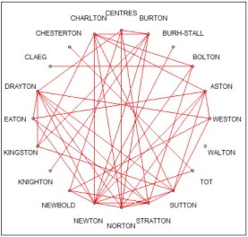
placenames based on K-cross functions. A line connecting two

place-names indicates that the deviation test described in Section 2.3.2 re-ports significant interaction when applied to the bivariateL-function

corresponding to such two placenames (see Section 2.3.2 for more

details). . . 17 2.8 Testing the null hypothesis of Section 2.3.3, based on Strauss point

processes, with the procedure described in Section 2.3.2. The

cen-tred L-function ˆLcross(r) −E[ ˆLcross(r)] for the observed pattern is

represented by (black) solid lines. The 95% envelopes (gray areas)

are obtained using 99 simulated patterns and the (red) dashed lines indicate the upper deviations. Deviation test: if the (black) solid line

rises above the (red) dashed line then the interaction can be

consid-ered significant at significance levelα= 0.05. . . 18

3.1 Estimate of the density function for the full dataset obtained through

Gaussian kernel smoothing (and truncation) with bandwidth chosen

using the functionbw.relriskfrom the Spatstat R package (Baddeley & Turner, 2005), which is based on the cross-validation method (see

e.g. Diggle, 2003, p.115-118). Edge correction has been performed

according to Diggle (1985). This function is used as an estimate of the probability densityg(·) of the center process z (Section 3.3). . . 24 3.2 Conditional independence structure of the random elements involved

in the Poisson Model. . . 31 3.3 Conditional independence structure of the random elements involved

in the Dirichlet-Multinomial model. . . 34

(9)

5.1 Average acceptance rates of the MH algorithm with proposals QU,

QT and QB for different values ofnand σ. . . 63 5.2 (a)-(c) Traceplots of a summary statistic defined asS(ρ) =Pn

i=1iρ(i).

(d) Distance from the target measure defined asD(T) =Pn i,j=1(ˆp

(T)

ij −

pij)2, where pij is the probability of {(i, j) ∈ ρ} under π(ρ)

(es-timated with a long MCMC run independently from the rest) and

ˆ

p(_ijT) = PT

t=11((i, j) ∈ ρt)/T, with (ρt)Tt=1 being the samples from

the MCMC algorithm under consideration. . . 64

6.1 Example of allowed moves induced by (6.1). In this case n1 = 3

and n2 = 2, where n1 and n2 are the number of red and blue points

respectively. Note that the index i in ρnew =ρold◦(i, j) refers to a

red point, while the indexj refers to a blue point. . . 79

6.2 Traceplots of the number of differences from a reference matching. . 84

6.3 The results of the diagnostic performed with four convergence diag-nostic techniques described in Section 6.1.3. . . 85

6.4 Configurations corresponding to local maxima of ˆπ(ρ) for (a) a syn-thetic sample and (b) an artificially designed configuration. . . 87

6.5 Left: the observed windowW divided into squares. Right: in this case

R1₁ ={1,3,4,5,7,9,17}andB₁1={3,4,6,7,8,9,10,11,13,16,18,19,21,24}. 90

6.6 Comparison of the multiple proposal scheme forl= 1,4,9 using the

convergence diagnostic techniques of Section 6.1.3. . . 92

6.7 The action of a transition kernel P(A) for a givenA. . . 94 7.1 (a) Estimated posterior distribution of p(₁c) (see Chapter 3) for the

reduced and full dataset (13 and 20 placenames respectively). The

hypothesis of no clustering (p(₁c) = 1) lies outside the support of the posterior for the real dataset. (b) Measure of association between

placenames (see end of Chapter 7). . . 99

7.2 (a) π(σ|x) for the reduced dataset. (b) π(σ|x) considering only a high-density region (see Chapter 8). . . 99

7.3 (a) Posterior distribution ofY= (Y1, . . . , Yk) for the reduced dataset.

(10)

7.4 Graphical representation of π(ρ|x), where x is the reduced dataset (13 placenames) in the whole observed region. The intensity of gray corresponds to the estimated posterior probability of the cluster. The

truncated kernel density estimation ofgis plotted in the background,

with values express in relative terms with respect to the uniform measure. . . 101

7.5 Comparison of the Dirichlet-Multinomial model (see Section 3.7.1)

and the Poisson one (see Section 3.5.1) on the reduced dataset in the high-density region. (a) Posterior distribution ofσ and (b) posterior

distribution ofY = (Y1, . . . , Yk) (see Section 3.7.1 for a definition of

Y). . . 103 7.6 Comparison of the posterior distributions of (a) p(₁c) and (b) σ,

ob-tained with and without the assumption of the marks being sampled

(11)

Acknowledgments

I would like to thank my supervisor, Wilfrid Kendall, for his generous availability

and constant support, for having put my professional growth ahead of his academic

interests and for his kindness and esteem towards me.

I am also grateful to many members of the Department of Statistics at the

University of Warwick: the countless number of colleagues who have been

avail-able to discuss the research of this thesis, the various friends, especially my fellow

PhD students, that contributed to make my time in the department enjoyable, and

finally the administrative staff for their prompt support with organizational and

bureaucratic issues.

I acknowledge John Blair for collaboration and arranging supply of data and

the Engineering and Physical Sciences Research Council for funding through the

(12)

Declarations

This thesis is submitted to the University of Warwick in support of my application

for the degree of Doctor of Philosophy. It has been composed by myself and has not

been submitted in any previous application for any degree.

The work presented was carried out by the author except where explicitly

indicated otherwise by references. Large part of the work in this thesis (excluding

Chapter 5) has formed the following paper:

Zanella, G. (2015) Random Partition Models and complementary clustering of

(13)

Abstract

Common cluster models for multi-type point processes model the aggregation of

points of the same type. In complete contrast, in the study of Anglo-Saxon

set-tlements it is hypothesized that administrative clusters involving complementary

names tend to appear. We investigate the evidence for such a hypothesis by

devel-oping a Bayesian Random Partition Model based on clusters formed by points of

different types (complementary clustering).

As a result we obtain an intractable posterior distribution on the space of

matchings contained in a k-partite hypergraph. We use the Metropolis-Hastings

(MH) algorithm to sample from such a distribution. We consider the problem of

what is the optimal, informed MH proposal distribution given a fixed set of allowed

moves. To answer such a question we define the notion of balanced proposals and

we prove that, under some assumptions, such proposals are maximal in the Peskun

sense. Using such ideas we obtain substantial mixing improvements compared to

other choices found in the literature. Simulated Tempering techniques can be used

to overcome multimodality and a multiple proposal scheme is developed to allow

for parallel programming. Finally, we discuss results arising from the careful use of

convergence diagnostic techniques.

This allows us to study a dataset including locations and placenames of 1316

Anglo-Saxon settlements dated around 750-850 AD. Without strong prior

knowl-edge, the model allows for explicit estimation of the number of clusters, the average

intra-cluster dispersion and the level of interaction among placenames. The results

support the hypothesis of organization of settlements into administrative clusters

(14)

Chapter 1

Introduction

The starting point of this work is a dataset supplied by John Blair of Queen’s College Oxford, Professor of History at the University of Oxford. The dataset consists of

the locations and placenames of 1316 Anglo-Saxon settlements dated approximately

around 750-850 AD. Professor Blair’s hypothesis is that those settlements were organized into administrative districts involving settlements with complementary

roles and that such roles were indicated by the different placenames (see Section

2.1).

If present, such a phenomenon would induce clusters of closely located

set-tlements with different placenames (complementary clustering). On the contrary,

typical cluster models for marked point processes deal with the aggregation of ele-ments of thesame type (or with similar features). In the latter case, one can treat

the marks/types as an additional dimension and perform clustering in a higher

di-mensional space (e.g. two spatial dimensions plus one marks dimension), while in our scenario the spatial dimensions and the marks/types dimension have different

roles. This has both modeling and computational implications.

We develop a Bayesian Random Partition Model (RPM) to study comple-mentary clustering phenomena. RPMs provide a general, flexible framework and

allow to make explicit inferences on the unobserved partition. Because of the

com-plementarity requirement, the posterior sample space uses the space of matchings contained in a k-partite hypergraph. We devote much attention to computational

aspects, both from the theoretical and practical point of view.

The model and algorithm we develop allow the study of the Anglo-Saxon set-tlements dataset. Without strong prior knowledge, the model allows for explicit

(15)

of organization of settlements into administrative clusters based on complementary

names and provide additional information and insight into such a phenomenon.

Thesis contributions

This work arises out of a specific applied problem presented to us by distinguished

historians. In trying to provide satisfactory answers to their questions, we develop

novel theory and methodology having wider implications, both from the modeling and especially from the computational point of view.

First we develop a Bayesian Random Partition Model tailored to study com-plementary clustering scenarios (see Chapter 3). Such a model may have

appli-cations to other scenarios (such as ecology, see e.g. Chapter 8) where clusters of

distinct elements occur, rather than clusters of similar objects. In particular two prior distributions (see Sections 3.5.1 and 3.7.1) are proposed to model clustering

scenarios with many small clusters with a bounded number of points each. We

de-scribe these models in terms of matchings contained in hypergraphs (Chapter 4), thus relating computational tasks to the Complexity Theory literature.

Secondly we study Markov chain Monte Carlo (MCMC) algorithms in

dis-crete spaces such as matchings contained in hypergraphs, in particular consider-ing the problem of designconsider-ing informed Metropolis-Hastconsider-ings (MH) proposals in such

spaces. Under some assumptions (satisfied by our model) we derive the class of

asymptotically optimal proposal distributions (Section 5.4). To prove such opti-mality we use the so-called Peskun ordering (Peskun, 1973), extending it to cases

involving a constant in the off-diagonal comparison (see Theorem 4). These results

motivate the introduction of the apparently new notion of balanced proposals (see Chapter 5). Such a notion provides a general and coherent way to incorporate

lo-cal information into MH proposal distributions and has the potential to extend the

benefits of gradient-based MCMC algorithms to discrete settings (see Section 8.3). Finally we describe practical implementations of the ideas in Chapter 5 for

the applied problem under consideration. We discuss various practical issues

(tem-pering, parallel computing, convergence diagnostic) and we study the Anglo-Saxon settlements dataset, managing to provide informative answers to the historians’

questions (Chapter 7).

Organization of the thesis

Chapter 2 is divided in two parts. The first part describes the historical problem,

(16)

second part contains a preliminary analysis of the dataset with traditional spatial

statistics tools such as K-cross functions. This exploratory analysis suggests that there is some attractive interaction between settlements with different placenames

and motivates further analysis.

In Chapter 3 we define a Bayesian RPM for complementary clustering sce-narios. Some attention is devoted to the choice of prior distribution for the

parti-tion. This is necessary because the commonly used prior distributions, such as the

Dirichlet Process prior, are not appropriate for this context, for example because they model situations with few big clusters, while our scenario leads to many small

clusters.

The posterior distribution induced by the model of Chapter 3 is intractable. To address this more precisely, in Chapter 4 we study the computational complexity

of tasks associated with such a posterior distribution by appealing to known results

from the Complexity Theory literature. To do so we exploit the fact that the poste-rior distribution is proportional to the weight of a corresponding matching contained

in a weighted k-partite hypergraph. We thus link the problems of sampling from

the posterior and finding the posterior mode (or the maximum likelihood estimator) to the more classical problems of Data Association and Optimal Assignment.

Given the results discussed in Chapter 4 we need to use approximate meth-ods to perform inferences on the posterior distribution of interest. Motivated by

the results recalled in Section 4.2.4, we use Monte Carlo methods and in particular

MCMC algorithms. In Chapter 5 we introduce MCMC methods, in particular the Metropolis-Hastings (MH) algorithm and some theoretical notions related to

mea-suring MCMC efficiency. Then we consider the problem of choosing the optimal

proposal distribution given a fixed set of allowed moves (in a fairly general frame-work). To solve such a problem we introduce the notions of balanced proposals and

we show that under some assumptions such a family of proposals is optimal in terms

of (asymptotic) Peskun ordering (see Theorems 4, 5 and 6).

In Chapter 6 we return to the applied problem and we describe the actual

MCMC algorithm we use to obtain approximate samples from the posterior of

inter-est. To do so we deal with sampling matchings contained in hypergraphs (a problem often encountered, for example, in Data Association problems) and we use ideas from

Chapter 5 to speed up such sampling process. We consider convergence diagnostic

issues, we explore the use of Simulated Tempering to overcome multimodality and we develop a multiple proposal scheme to allow for parallel computation.

In Chapter 7 we analyze the Anglo-Saxon settlements dataset, fitting the

(17)

sup-port the hypothesis of settlements being organized into administrative clusters and

provide explicit inferences of various quantities of historical interest.

Finally in Chapter 8 we summarize the results and discuss possible

(18)

Chapter 2

Historical problem and

preliminary analysis

2.1 The historical question under consideration

As already mentioned in Chapter 1, the starting point of this work is the

Anglo-Saxon settlements dataset provided by Professor John Blair, which contains the locations and placenames of more than a thousand settlements. In the dataset there

are 20 different kinds of placenames in total. Placenames form an important source

of information regarding the Anglo-Saxon civilization and are intensively studied by the historical community (see for example Gelling & Cole, 2000 and Jones &

Semple, 2012).

In particular, the placenames included in this dataset are often described asfunctional placenames, as they were probably used to indicate specific functions

or features of their corresponding settlements. For example Burton is thought to

label fortified settlements having a military role, Charlton the settlements of the peasants andDraytonthe settlements dedicated to portage.

Moreover, historians expect the settlements in this dataset (especially those

having one of the placenames underlined in Table 2.1) to have been formed approx-imately at the same time and in the same context (specifically, royal administration

in the period c.750-850). This suggests that there could be some coherence in the distribution of such placenames. In particular Professor Blair’s hypothesis is that

those settlements were not independent units but rather that they were organized

into administrative clusters (or districts) where placenames were used to indicate the role of each settlement within the district. According to this hypothesis such

(19)

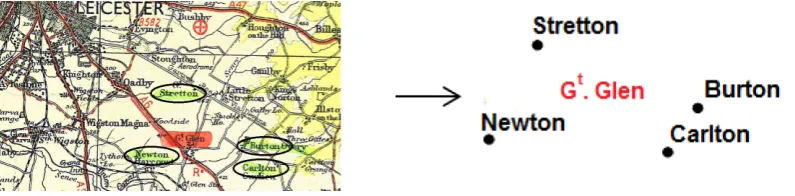
them. For example Figure 2.1 indicates a plausible administrative cluster made of

[image:19.595.123.521.166.264.2]

four settlements, with, for example, a settlement dedicated to military functions (Burton) and one dedicated to agriculture (Carlton).

Figure 2.1: A cluster of four Anglo-Saxon settlements (circled and highlighted in green) in the region of Great Glen (written in short as Gt.Glen).

The objective of our statistical approach to the study of settlements names

and geographical locations is to address the following questions: is there statistical support for Blair’s hypothesis? What is the typical distance between settlements in

the same cluster? How many settlements are clustered together and how many are

singletons? Which placenames tend to cluster together? Can we provide a list of those clusters that are more strongly supported by the analysis?

Our intention is to provide a useful contribution to historical research on this topic based on a quantitative approach, bearing in mind the scarcity of textual

evidence regarding the Anglo-Saxon period. Since there is much uncertainty and

controversy regarding the meaning of placenames, even the apparently obvious ones, we should try to be fairly neutral from the historical point of view, avoiding strong

assumptions on the functions of placenames and relationships among them. This will

help our statistical analysis to be a genuine contribution to the ongoing historical debate on this topic.

We note that there has already been statistical work related to Anglo-Saxon

placenames. In particular see the work of Keith Briggs on this topic (see http: //keithbriggs.info/place-names.htmlfor a full list). Nevertheless both the his-torical questions considered and the statistical methodologies used are substantially

different from ours.

2.2 The AngloSaxon settlements dataset

We now describe the Anglo-Saxon settlements dataset supplied by Prof. John Blair and the data cleaning operations that we carried out. The dataset (fully available

(20)

is made of 20 different groups, each of which contains the list of settlements having

one of the 20 placenames (see Table 2.1). The historians involved in the project

Placenames total # of settlements # of couples # of couples number with less precise (as classified (as classified location by historians) by proximity)

Aston/Easton 90 0 1 8

Bolton 17 1 1 0

Burh-Stall 29 2 1 0

Burton 108 2 1 7

Centres 46 0 0 0

Charlton/Charlcot 98 3 7 1

Chesterton 9 0 0 0

Claeg 84 13 0 5

Draycot/Drayton 55 1 0 2

Eaton 33 1 1 5

Kingston 71 1 1 1

Knighton 26 1 0 0

Newbold 34 3 1 0

Newton 191 5 4 5

Norton 74 1 8 1

Stratton 37 0 5 0

Sutton 101 2 4 5

Tot 77 17 1 1

Walton/Walcot 51 4 1 0

Weston 85 3 3 2

[image:20.595.133.509.150.453.2]

Total 1316 60 40 43

Table 2.1: Number of settlements in the Anglo-Saxon placenames location dataset supplied by Prof. Blair. The historians expect the clustering behavior mainly to involve 13 of those placenames (underlined and emboldened in this table). Settle-ments with less precise locations (third column) are settleSettle-ments whose location is given with 1 km accuracy, rather than 100 m, or having a more uncertain location (see Section 2.2). The term “couples” (last two columns) refers to multiple records of the same settlements (see Section 2.2.1 for discussion). The “total number” column refers to the count after merging the couples classifieds by historians.

expect the clustering behavior to involve 13 of those placenames in particular, indi-cated in Table 2.1. We refer to the settlements relative to those 13 placenames as

thereduced dataset, and to all the settlements recorded as the full dataset. We will

perform statistical analyses on both datasets.

For each settlement the following variables are given: County, place, Parish

or Township, grid ref and date of first evidence (see Table 2.2).

(21)

PARISH OR GRID DATE OF

COUNTY PLACE TOWNSHIP REF FIRST

EVIDENCE

BRK Bourton Bourton SU 230870 c. 1200

BUC Bierton Bierton with Broughton SP 836152 DB

BUC Bourton Buckingham SP 710333 DB

CHE Burton Burton (T) SJ 509639 DB

CHE Burton Burton (T) SJ 317743 1152

[image:21.595.135.509.107.230.2]

CHE Buerton Buerton (T) SJ 682433 DB

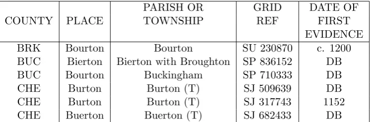
Table 2.2: Exemplary data available for the first 6 settlement with the nameBurton. The acronym DB stands for Domesday Book, compiled in 1086.

identify a 100m×100m square on a grid covering Great Britain. Some locations

have just 2 letters and 4 digits (e.g.SU2387) and they identify a 1km×1km square,

and some have a letter c in front of them (e.g. c.SU2387) to indicate that the location is less accurate (see Table 2.1 for amounts of these).

2.2.1 Data cleaning and data assumptions

Our analysis is concerned with placenames (variable “place”) and geographical lo-cations (variable “Grid reference”). By considering placenames as marks attached

to points, we model our data as the realization of ak-type point process (also called

k-variate point process), where k is the number of different placenames available (see Baddeley, 2010 or Section 2.3 for more details on point processes). We convert

the data to a k-type point process form as described below. This data cleaning

process entails historical assumptions on the dataset and thus we have been guided by the judgment of the subject-specific historians involved in this project in doing

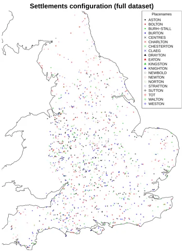
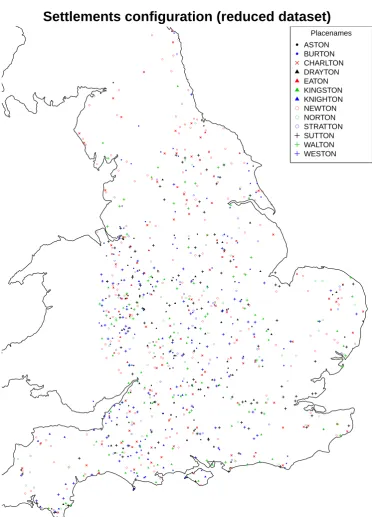
so. Figure 2.2 shows the resulting k-type point pattern for the full dataset, while

Figure 2.3 shows that only for the reduced dataset.

Placenames: we express the variable “place” as a categorical variable withk

possible values (i.e.ktypes). For the full datasetkequals 20, while for the reduced

datasetkequals 13. By describing the variable “place” as a categorical variable we ignore minor variations in placenames. For example we consider all the settlements

of Table 2.2 as having placename Burton: their actual recorded placenames vary

amongstBurton, Bourton, Bierton, Buerton.

Four groups (out of 20) are made up of two subgroups each with similar

place-names: Aston/Easton,Charlton/Charlcot,Drayton/DraycotandW alton/W alcot. We consider placenames within such subgroups to be the same, for exampleCharlton

(22)

● ● ● ● ● ● ● ● ● ● ● ● ● ● ● ● ● ● ● ● ● ● ● ● ● ● ● ● ● ● ● ● ● ● ● ● ● ● ● ● ● ● ● ● ● ● ● ● ● ● ● ● ● ● ● ● ● ● ● ● ● ● ● ● ● ● ● ● ● ● ● ● ● ● ● ● ● ● ● ● ● ● ● ● ● ● ● ● ● ● ● ● ● ● ● ● ● ● ● ● ● ● ● ● ● ● ● ● ● ● ● ● ● ● ● ● ● ● ● ● ● ● ● ● ● ● ● ● ● ● ● ● ● ● ● ● ● ● ● ● ● ● ● ● ● ● ● ● ● ● ● ● ● ● ● ● ● ● ● ● ● ● ● ● ● ● ● ● ● ● ● ● ● ● ● ● ● ● ● ● ● ● ● ● ● ● ● ● ● ● ● ● ● ● ● ● ● ● ● ● ● ● ● ● ● ● ● ● ● ● ● ● ● ● ● ● ● ● ● ● ● ● ● ● ● ● ● ● ● ● ● ● ● ● ● ● ● ● ● ● ● ● ● ● ● ● ● ● ● ● ● ● ● ● ● ● ● ● ● ● ● ● ● ● ● ● ● ● ● ● ● ● ● ● ● ● ● ● ● ● ● ● ● ● ● ● ● ● ● ● ● ● ● ● ● ● ● ● ● ● ● ● ● ● ● ● ● ● ● ●● ● ● ● ● ● ● ● ● ● ● ● ● ● ● ● ● ● ● ● ● ● ● ● ● ● ● ● ● ● ● ● ● ● ● ● ● ● ● ● ● ● ● ● ● ● ● ● ● ● ● ● ● ● ● ● ● ● ● ● ● ● ● ● ● ● ● ● ● ● ● ● ● ● ● ● ● ● ● ● ● ● ● ● ● ● ● ● ● ● ● ● ● ● ● ● ● ● ● ● ● ● ● ● ● ● ● ● ● ● ● ● ● ● ● ● ● ● ● ● ● ● ● ● ● ● ● ● ● ● ● ● ● ● ● ● ● ● ● ● ● ● ● ● ● ● ● ● ● ● ● ● ● ● ● ● ● ● ● ● ● ● ● ● ● ● ● ● ● ● ● ● ● ● ● ● ● ● ● ● ● ● ● ● ● ● ● ● ● ● ● ● ● ● ● ● ● ● ● ● ● ● ● ● ● ● ● ● ● ● ● ● ● ● ● ● ● ● ● ● ● ● ● ● ● ● ● ● ● ● ● ● ● ● ● ● ● ● ● ● ● ● ● ● ● ● ● ● ● ●

Settlements configuration (full dataset)

[image:22.595.119.495.106.623.2]

● ● ● ● ● ● ● ● Placenames ASTON BOLTON BURH−STALL BURTON CENTRES CHARLTON CHESTERTON CLAEG DRAYTON EATON KINGSTON KNIGHTON NEWBOLD NEWTON NORTON STRATTON SUTTON TOT WALTON WESTON

(23)

● ● ● ● ● ● ● ● ● ● ● ● ● ● ● ● ● ● ● ● ● ● ● ● ● ● ● ● ● ● ● ● ● ● ● ● ● ● ● ● ● ● ● ● ● ● ● ● ● ● ● ● ● ● ● ● ● ● ● ● ● ● ● ● ● ● ● ● ● ● ● ● ● ● ● ● ● ● ● ● ● ● ● ● ● ● ● ● ● ● ● ● ● ● ● ● ● ● ● ● ● ● ● ● ● ● ● ● ● ● ● ● ● ● ● ● ● ● ● ● ● ● ● ● ● ● ● ● ● ● ● ● ● ● ● ● ● ● ● ● ● ● ● ● ● ● ● ● ● ● ● ● ● ● ● ● ● ● ● ● ● ● ● ● ● ● ● ● ● ● ● ● ● ● ● ● ● ● ● ● ● ● ● ● ● ● ● ● ● ● ● ● ● ● ● ● ● ● ● ● ● ● ● ● ● ● ● ● ● ● ● ● ● ● ● ● ● ● ● ● ● ● ● ● ● ● ● ● ● ●● ● ● ● ● ● ● ● ● ● ● ● ● ● ● ● ● ● ● ● ● ● ● ● ● ● ● ● ● ● ● ● ● ● ● ● ● ● ● ● ● ● ● ● ● ● ● ● ● ● ● ● ● ● ● ● ● ● ● ● ● ● ● ● ● ● ● ● ● ● ● ● ● ● ● ● ● ● ● ● ● ● ● ● ● ● ● ● ● ● ● ● ● ● ● ● ● ● ● ● ● ● ● ● ● ● ● ● ● ● ● ● ● ● ● ● ● ● ● ● ● ● ● ● ● ● ● ● ● ● ● ● ● ● ● ● ● ● ● ● ● ● ● ● ● ● ● ● ● ● ● ● ● ● ● ● ● ● ● ● ● ● ● ● ● ● ● ● ● ● ● ● ● ● ● ● ● ● ● ● ● ● ● ● ● ● ● ● ● ● ● ● ● ● ● ● ● ● ● ● ● ● ● ● ● ● ● ● ● ● ● ● ● ● ● ● ● ● ● ● ● ● ● ● ● ● ● ● ● ● ● ● ● ● ● ● ● ● ● ● ● ● ● ● ● ● ● ● ● ●

Settlements configuration (reduced dataset)

[image:23.595.121.494.102.620.2]

● ● ● ● ● Placenames ASTON BURTON CHARLTON DRAYTON EATON KINGSTON KNIGHTON NEWTON NORTON STRATTON SUTTON WALTON WESTON

(24)

Figure 2.4 provides a box-plot representation of the observedx and y

coor-dinates divided by placenames. Such a plot provides a crude representation of the variability in the distribution of settlements across different placenames. Note that,

especially for the reduced dataset (represented with black solid lines in Figure 2.4),

there is no clear suggestion of grouping. In fact, for most couples of placenames, sayAandB, the area with a high density of settlements of typeA has a consistent

overlap with that of settlements of type B. Therefore, it does not seem

appropri-ate to divide placenames into groups and to analyze the corresponding settlements separately.

We will not model the heterogeneity in placenames distribution explicitly

in the cluster analysis (see Section 8.2 for discussion of possible improvements). Note, however, that we do model such heterogeneity in the null-hypothesis testing

of Section 2.3.2 and the sanity check of Section 7.1.

Locations: we convert OS National Grid coordinates to two-dimensional Eu-clidean coordinates and each settlement is assumed to be located at the center of

the corresponding OS National Grid square.

Multiple records: it is sometimes indicated in the original dataset that some couples (or triples) of settlements, with the same placename and very close locations,

have to be considered as multiple records of the same settlement. We replaced such couples (or triples) of settlements with a single settlement located at their midpoint.

Moreover there are some other pairs of records having very close locations and the

same placename (see Table 2.1 for amounts). It is primarily a matter of historical interpretation whether these couples have to be considered as single settlements. We

performed the analysis under both hypotheses (keeping them separated or merged)

without seeing significant changes in the results. The analysis presented here is made with those settlements merged together (3 km is the threshold distance below

which we identify two records of settlements with the same placename).

Observation regionW: a point process realization consists of point locations and of the region W where the points have been observed. Indeed both the

K-cross function analysis of Section 2.3.1 and the Bayesian model of Chapter 3 will

use information about W. In our case we define W as Great Britain (coastline obtained from the mapdata R package Becker et al. , 2013) cropping the region

where the point process intensitygfalls below a certain threshold, approximately at

the borders between England-Scotland and England-Wales. We also added a small buffer zone of 3 km around the region to include the few points that were falling

outside the region (e.g. because the coastline has moved or because the location was

(25)

[image:25.595.123.518.102.599.2]

(26)

2.3 Preliminary analysis of the Anglo-Saxon settlements

dataset

We now perform preliminary analysis on the resulting point pattern using classic Spatial Statistic tools. As mentioned before, we can model the data as the realization

of aspatial point process. Spatial point processes are random configuration of points

in the plane, or more precisely stochastic processes whose realizations consist of a finite (or countably infinite) set of points contained in some window W ⊆_R2_{. For}

simplicity we assume the number of points to be finite and all the points to have distinct locations (i.e. no two points are allowed to be one on top of the other). We

denote a realization of a spatial point process byx={x1, . . . , xn(x)}. Note that the

set of points is unordered and that the number of points is not fixed.

The most important example of point process is thePoisson point process.

A point process x is a Poisson point process driven by an intensity measure Λ(·), with Λ(·) being a measure onW ⊆_R2_{, if for any measurable}_A_⊆_W _{the number of}

points ofxbelonging toA is a random variable which follows a Poisson distribution with mean Λ(A). The importance of the Poisson point process is due to the fact

that it is the only possible model where points are completely independent of each other, meaning that, givenA1 andA2disjoint subsets ofW, the number of points in

A1 and A2 are independent random variables. See Daley & Vere-Jones (2002) and

Daley & Vere-Jones (2008) for a rigorous introduction to point processes in terms of random discrete measures.

Another important class of models is the class of cluster point processes.

Such point processes are built in two stages: first a set of “parents” (or “centers”) is generated and then, for each center, a “daughter” point process (or “cluster”)

is generated. The cluster point process is then defined as the superposition of all

the daughter point processes. Cluster point processes are typically used to model scenarios where the clusters consist of the aggregation of closely located points. See

Chiuet al. (2013) and Isham (2010) for more details on models for spatial point

processes.

2.3.1 K-cross function analysis

Second moment functions are a useful tool to investigate inter-point interaction (e.g.

Chiu et al. , 2013). In particular, given a multi-type point pattern, bivariate (or cross-type) K-functions provide good summary functions of the interaction across

points of different types. The bivariate K-functionKij(r) is the expected number of

(27)

of the typej sub-pattern of pointsxj (e.g. Baddeley, 2010, Sec. 6). For testing and

displaying purposes we define a single summary function, a multi-type K-function

Kcross(r), as the weighted average of Kij(r) for i 6= j, where the weights are the

product of the intensitiesλiλj.

Classical K-functions, however, rely strongly on the assumption that the point pattern is stationary, which is not appropriate for our dataset. Therefore we

use the inhomogeneous version of the K-functions, where the contribution coming

from each couple of points is reweighted to account for spatial inhomogeneity (Bad-deleyet al., 2000). Standard estimates of the inhomogeneous bivariateK-functions

ˆ

Kij are obtained using thespatstat R package (Baddeley & Turner, 2005).

2.3.2 Null hypothesis testing

In order to test whether the interaction shown byK-functions is significant or not

we need to define a null hypothesis (representing no-interaction among placenames).

Section 8 of Baddeley (2010) describes three classical null hypotheses for multivari-ate point processes: random labeling (given the locations the point types are i.i.d.),

Complete Spatial Randomness and Independence (CSRI, the locations arise from a

uniform Poisson point process and the point types are i.i.d.) and independence of components (points of different types are independent). The random labeling and

the CSRI hypotheses are unrealistic assumptions for our dataset because our point

pattern is clearly not stationary and the distribution of placenames is not spatially homogeneous (some placenames are more concentrated in the South, some in the

North and so on). The independence of components hypothesis is realistic but, in

order to test it, stationarity of the points pattern is usually assumed. Instead we define the following no-interaction null hypothesis: each sub-pattern of pointsxj is

an inhomogeneous Poisson point process (with intensity function λj(·) potentially

varying over j). Note that a more realistic null hypothesis would also include re-pulsion among points of the same type. In Section 2.3.3 we implement such a null

hypothesis using Strauss point-processes. The results are very similar to the ones

presented here.

Given the null hypothesis we perform the following approximate Monte Carlo

test. First we estimate the intensities λj(·) with ˆλj(·) (see Figures 2.5) obtained

through standard Gaussian kernel smoothing with bandwidth chosen according to the cross-validation method (e.g. Diggle, 2003, p.115-118), and edge correction

performed according to Diggle (1985). The cross-validation method considers, for each pointxi, the density function estimated using all points apart fromxievaluated

(28)

[image:28.595.123.505.103.564.2]

Figure 2.5: Estimates of the intensity function for each placename obtained through Gaussian kernel smoothing (and truncation) with bandwidth chosen using the

func-tion bw.relrisk from the Spatstat R package (Baddeley & Turner, 2005), which

is based on the cross-validation method (see for example Diggle, 2003, p.115-118). Edge correction is performed according to Diggle (1985). The color scales are dif-ferent for each placename, but they all start from 0. These estimates are used in Section 2.3.1 to simulate synthetic samples from the no-interaction null hypothesis.

given the intensity estimates, we sample 99 independent multivariate inhomogeneous

Poisson point patterns according toλˆj(·) k

(29)

simulation envelopes and to perform a deviation test with significanceα= 0.05 using

as a summary function a centered version of the L-function ˆLcross(r) =

q

ˆ

Kcross(r)

π

forr ∈(0, rmax), with rmax = 15km. The deviation test (Grabarniket al. , 2011)

summarizes the summary function with a single valueD= maxr∈(0,rmax)Lˆcross(r)−

E[ ˆLcross(r)] and compares it to the ones obtained from the 99 simulated samples.

0 5 10 15

−0.5

0.5

1.5

Envelopes and deviation test for the full Dataset

r [km]

Centered L−cross function −0.5 0 5 10 15

0.5

1.5

Envelopes and deviation test for the reduced Dataset

r [km]

[image:29.595.124.510.201.332.2]

Centered L−cross function

Figure 2.6: The centredL-function ˆLcross(r)−E[ ˆLcross(r)] for the observed pattern

is represented by (black) solid lines, the 95% envelopes (gray areas) are obtained using 99 simulated patterns and the (red) dashed lines indicate the upper deviations. Deviation test: if the (black) solid line rises above the (red) dashed line then the interaction can be considered significant at significance levelα= 0.05. The values of

E[ ˆLcross(r)] are estimated using independently simulated point patterns generated

according to the null hypothesis.

The null hypothesis is rejected for both the full and the reduced dataset (see

Figure 2.6). For the reduced dataset this provides evidence of a stronger cluster-ing effect. The R code used to perform this test and produce Figure 2.6 is given

at https://sites.google.com/site/gzanellawebpage/compclust_supp_f.zip. Application of the same deviation test on the bivariateL-functions ˆLij(r) provides

an indication of which couples of placenames exhibit significant interaction (see

Figure 2.7). Such a plot allows historians to compare the interaction reported by

theK-function analysis with historical hypotheses and contextual information (see Section 7.1 for more details).

2.3.3 Null-hypothesis using Strauss point processes

In Section 2.3.2 we defined the following null hypothesis for the distribution of the

marked point process x under consideration: each point pattern x(j) is an inho-mogeneous Poisson point process with intensity function λj(·). Here x(j) denotes

(30)

[image:30.595.181.459.121.385.2]

Figure 2.7: Graphical representation of significant pairwise interaction among place-names based on K-cross functions. A line connecting two placeplace-names indicates that the deviation test described in Section 2.3.2 reports significant interaction when ap-plied to the bivariateL-function corresponding to such two placenames (see Section 2.3.2 for more details).

it is reasonable to expect settlements with the same placename not to be too close

to each other. This could be modeled by assuming that each point pattern xj is

distributed according to an inhomogeneous Strauss process, andx(j) is independent fromx(i) foridifferent fromj. A Strauss point processx(j)={x(₁j), . . . , x(_nj₍)_x

j)}has

probability density function

f(x(j)) =α γs(x(j))

n(x(j)₎

Y

i=1

λj(x(ij)),

with respect to the distribution of a unitary homogeneous Poisson point process

(in a Radon-Nikodym derivative sense). Here α is a normalizing constant, γ is a

inhibition parameter between 0 and 1,s(x(j)) is the number of (unordered) couples of points in x(j) closer than some distance R > 0 apart, and λj(·) is the intensity

function. See Chiuet al. (2013) for more rigorous definitions of the Strauss process

(31)

We then perform the same approximate Monte Carlo test of Section 2.3.2,

replacing the inhomogeneous Poisson point process model with the Strauss one (the estimated intensities ˆλj(·) are obtained as in Section 2.3.2). In order to perform

such a test we need to choose the values of the inhibition parameter γ and the

maximal inhibition distanceR determining the distribution of the Strauss process. We considered γ equal to 0.1, 0.5 and 0.9 (corresponding to strong, medium and

mild interaction). Given the historical context we considered values of the inhibition

0 5 10 15

−0.5

0.5

1.5

Envelopes and deviation test for the full Dataset (Strauss)

r [km]

Centered L−cross function −0.5 0 5 10 15

0.5

1.5

Envelopes and deviation test for the reduced Dataset (Strauss)

r [km]

[image:31.595.125.511.234.365.2]

Centered L−cross function

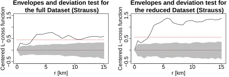
Figure 2.8: Testing the null hypothesis of Section 2.3.3, based on Strauss point processes, with the procedure described in Section 2.3.2. The centred L-function

ˆ

Lcross(r)−E[ ˆLcross(r)] for the observed pattern is represented by (black) solid lines.

The 95% envelopes (gray areas) are obtained using 99 simulated patterns and the (red) dashed lines indicate the upper deviations. Deviation test: if the (black) solid line rises above the (red) dashed line then the interaction can be considered significant at significance levelα= 0.05.

distanceR equal to 5, 10 and 20 km. We tried all the 9 resulting combinations ofγ

and R. The results did not change significantly from the ones obtained in Section 2.3.2 using the inhomogeneous Poisson point process model. Figure 2.8 shows the

result obtained usingγ = 0.1 andR= 20 (the strongest interaction among the ones

we considered). It can be seen that the 95% envelopes with such a null hypothesis are very similar to the ones obtained in Section 2.3.2. Note that one could try to

estimate R and γ from the data. We did not consider such estimation process to

be necessary at this stage, as the effect of introducing repulsion among same-type points did not impact the results of the null-hypothesis test.

2.3.4 Conclusion from the preliminary analysis

Our preliminary analysis indicates a clustering interaction between points of different types. NeverthelessK-functions do not provide explicit estimates and quantification

(32)

In the next Chapter we develop a Random Partition Model in order to provide more

informative answers to the questions of historical interest. We regardK-functions as a useful exploratory tool and the fact that they indicate interaction is a motivation

to pursue further statistical analysis.

We understand that Dr. Stuart Brookes from UCL has already used second moment functions to do some preliminary analysis on the Anglo-Saxon settlements

(33)

Chapter 3

A Bayesian complementary

clustering model

3.1 Overview of possible modeling approaches

We can view our problem as a clustering problem based on aggregations of points

of different types. In fact we seek a complementary clustering: each cluster may contain at most one settlement for each placename. This simplifying requirement

is motivated by the assumption that each placename represents a different

admin-istrative function (role) within the cluster (see Section 2.1). Note that the use of a clustering model is motivated by the historians’ belief that settlements were

orga-nized into administrative units that can be represented by clusters. See Section 8.2

for a discussion of some alternative modeling approaches.

Our intention is to perform explicit inferences on the partition of settlements

into clusters. As with hierarchical models, it would be desirable to analyze the

dataset all at once, so at not to lose statistical power, and also to provide inferences at the single cluster level to facilitate visualization and historical interpretation of

the results of the analysis.

We employ Random Partition Models (RPMs), often used in the Bayesian Nonparametric literature (e.g. Lau & Green, 2007), as they permit natural inferences

on the cluster partition and they have enough flexibility to allow specification of a useful model for complementary clustering.

Standard approaches for point process cluster modeling, like the Log-Gaussian

Cox Processes (see Lawson & Denison, 2010, Ch.3) or the Neyman-Scott model (e.g. Loizeaux & McKeague, 2001), are not appropriate here, as such models usually

(34)

seek explicit inferences on the cluster partition. Moreover standard cluster

meth-ods for marked point process consider the marks as an additional dimension and search for aggregations of points with similar marks. In complete contrast, we seek

aggregations of points of different types.

Diggle et al. (2006) seek evidence for repulsion among points of different types in a bivariate spatial distribution of amacrine cells. They use a pairwise

interaction model, which has theoretical limitations preventing its use for clustering.

While this approach could be extended to our case by using area-interaction point processes, which can model clustering (Baddeley & Van Lieshout, 1995), it would

not provide us with explicit estimates of the cluster partition and it would not easily

allow complementary clustering specification (at most one point of each type in each cluster).

Multi-target tracking involves the Data Association problem, that is to group

together measurements recorded at different time intervals to create objects tracks (e.g Ohet al., 2009). This problem is similar to the problem of performing

comple-mentary clustering of ak-type point process. In Data Association problems,

how-ever, the interest is to find the best association, while we are interested in assessing the strength of clustering and the level of interaction between different placenames,

and in quantifying the uncertainty of our estimates. In fact the modeling aspects we have to be careful about are different from the ones of Data Association problems,

though the computational challenges are similar (see Chapters 4 and 6).

3.2 Random Partition Models

We present Random Partition Models (RPMs) in the specific context of planar k

-type point processes. For more general and detailed discussions see Lau & Green

(2007) and M¨uller & Quintana (2010). Let ρ be a partition of an ordered set of marked points x = (x1, m1), . . . ,(xn(x), mn(x))

, with each (xi, mi)

belong-ing to R2 × {1, . . . , k}. Thus ρ can be represented as an unordered collection

{C1, . . . , CN(ρ)} of disjoint non-trivial subsets of the indices {1, . . . , n(x)} whose

union is the whole set {1, . . . , n(x)}. RPMs are used to draw inferences on the partitionρ given the observed pointsx. GivenCj =

n

i(₁j), . . . , i(sjj)

o

we define

xCj =

x_i(j) 1

, m_i(j) 1

, . . . ,

x_i(j) sj , mi(j)sj

for j running from 1 to N(ρ). We call xCj cluster and sj the size of the cluster.

(35)

independently of locations in other clusters, according to a probability density

func-tionh(sj,σ)(·) depending onsj and on a global intra-cluster dispersion parameterσ.

Thus the probability density function of x conditional onρ and σ is

π(x|ρ, σ) ∝

N(ρ)

Y

j=1

h(sj,σ)(xCj).

We assign independent prior distributions to ρ and σ. With a slight abuse

of notation, we denote them byπ(ρ) andπ(σ) respectively. We requireπ(ρ) to be exchangeable with respect to the point indices{1, . . . , n(x)} to reflect the fact that point labels are purely arbitrary and have no specific meaning. This is a common

requirement in the RPMs literature. We obtain the following expression for the posterior density function

π(ρ, σ|x) ∝ π(ρ)π(σ)

N(ρ)

Y

j=1

h₍_s_j_,σ₎(xCj).

3.3 Likelihood function

Givenρandσ, each clusterxCj is constructed as follows. First an unobserved center

point zj is sampled from the observation region W ⊆ R2 with probability density

functiong(·). Then the observed points x

i(j)₁ , . . . , xi(j)_sj are given by

x_i(j) l

=zj+y_i(j) l

, l= 1, . . . , sj (3.1)

wherey_i(j) l

is defined as

y

i(j)_l = wi(j)_l −

1

sj sj

X

l=1

w

i(j)_l

with w_i(j) 1

, . . . , w_i(j)

sj being independent bivariate N(0,

σ2

π I2) random vectors, where

I2 is the 2×2 identity matrix. The variance parametrization σ

2

π is chosen so thatσ

equals the expected distance between two points in the same cluster, independently

of the value ofsj. In fact ifx1 and x2 belong to the same cluster it holds

E

q

(x1−x2)>(x1−x2)

=E

q

(w1−w2)>(w1−w2)

=

r

π

2 r

2σ2

(36)

wherea>a=P2

i=1a2i forainR2, and we used the fact that the euclidean norm of

a two dimensionalN(0, η2I2) random vector follows the Rayleigh distribution and

its mean equalsp_π

2η forη≥0.

Finally the marksm

i(j)1

, . . . , m

i(j)_sj are sampled uniformly from the set

M_s_j =

(m1, . . . , msj)|ml∈ {1, . . . , k} and ml1 6=ml2 forl1 6=l2 .

The resulting likelihood function is

h₍_s_j_,σ₎(xCj) =

g xCj

Q

l1,l2∈Cj;l16=l21(ml1 6=ml2)

k!

(k−sj)!sj (2σ

2₎sj−1 exp

−πδ

2

Cj

2σ2

!

, (3.2)

wherexCj is the Euclidean barycenter ofxCjandδ

2

Cj =

P

i∈Cj xi−xCj

>

xi−xCj

. Section 3.3.1 below provides detailed calculations to obtain (3.2).

Note that in this section we are treatingg(·) as a known function. For the purposes of data analysis we will replace g with an estimate ˆg. Note that this

re-placement commits us to the use of a data-driven prior. The estimate ˆg (see Figure

3.1) is obtained using Gaussian kernel smoothing with bandwidth chosen accord-ing to the cross-validation method (Diggle, 2003, p.115-118) and edge correction

performed according to Diggle (1985). See Section 2.3.1 for more details on the

cross-validation method.

Remark 1. Given the heterogeneity in the number of settlements across different placenames, the assumption of the marks being sampled uniformly seems not to be

very realistic. In Section 3.7.2 we propose an empirical Bayes approach to include

non-uniformity of marks in the model while maintaining computational feasibility and we present inferences under that assumption. Here we retain the uniform marks

assumption for simplicity and because the two approaches produce similar inferences.

Moreover the inferences with the uniform marks assumption are more conservative (see Section 7.2) and therefore preferable in this context.

Remark 2. This model does not constrain x_i(j) l

=zj+y_i(j) l

to lie in the observation regionW. To make the model more realistic one could condition the distribution of

y_i(j) l

in(3.1)onzj+y_i(j) l

∈W (which would be an additional form of edge-correction).

Nevertheless in our application the density function g is not concentrated on the

borders (apart from the England-Wales border) and the values ofσ are small (below

10 kilometers) compared to the size of W. Therefore most correction terms would be negligible. Moreover computing a correction term for each center point zj would

(37)

0.0e+00 2.0e−06 4.0e−06 6.0e−06 8.0e−06 1.0e−05 1.2e−05 1.4e−05

Density estimation for the full dataset

[image:37.595.120.517.101.566.2]

● ● ● ● ● ● ● ● ● ● ● ● ● ● ● ● ● ● ● ● ● ● ● ● ● ● ● ● ● ● ● ● ● ● ● ● ● ● ● ● ● ● ● ● ● ● ● ● ● ● ● ● ● ● ● ● ● ● ● ● ● ● ● ● ● ● ● ● ● ● ● ● ● ● ● ● ● ● ● ● ● ● ● ● ● ● ● ● ●● ● ● ● ● ● ● ● ● ● ● ● ● ● ● ● ● ● ● ● ● ● ● ● ● ● ● ● ● ● ● ● ● ● ● ● ● ● ● ● ● ● ● ● ● ● ● ● ● ● ● ● ● ● ● ● ● ● ● ● ● ● ● ● ● ● ● ● ● ● ● ● ● ● ● ● ● ● ● ● ● ● ● ● ● ● ● ● ● ● ● ● ● ● ● ● ● ● ● ● ● ● ● ● ● ● ● ● ● ● ● ● ● ● ● ● ● ● ● ● ● ● ● ● ● ● ● ● ● ● ● ● ● ● ● ● ● ● ● ● ● ● ● ● ● ● ● ● ● ● ● ● ● ● ● ● ● ● ● ● ● ● ● ● ● ● ● ●● ● ● ● ● ● ● ● ● ● ● ● ● ● ● ● ● ● ● ● ● ● ● ● ● ● ● ● ● ● ● ● ● ● ● ● ● ● ● ● ● ● ● ● ● ● ● ● ● ● ● ● ● ● ● ● ● ● ● ● ● ● ● ● ● ● ● ● ● ● ● ● ● ● ● ● ● ● ● ● ● ● ● ● ● ● ● ● ● ● ● ● ● ● ● ● ● ● ● ● ● ● ● ● ● ● ● ● ● ● ● ● ● ● ● ● ● ● ● ● ● ● ● ● ● ● ● ● ● ● ● ● ● ● ● ● ● ● ● ● ● ● ● ● ● ● ● ● ● ● ● ● ● ● ● ● ● ● ● ● ● ● ● ● ● ● ● ● ● ● ● ● ● ● ● ● ● ● ● ● ● ● ● ● ● ● ● ● ● ● ● ● ● ● ● ● ● ● ● ● ● ● ● ● ● ● ● ● ● ● ● ● ● ● ● ● ● ● ● ● ● ● ● ● ● ● ● ● ● ● ● ● ● ● ● ● ● ● ● ● ● ● ● ● ● ● ● ● ● ● ● ● ● ● ● ● ● ● ● ● ● ● ● ● ● ● ● ● ● ● ● ● ● ● ● ● ● ● ● ● ● ● ● ● ● ● ● ● ● ● ● ● ● ● ● ● ● ● ● ● ● ● ● ● ● ● ● ● ● ● ● ● ● ● ● ● ● ● ● ● ● ● ● ● ● ● ● ● ● ● ● ● ● ● ● ● ● ● ● ● ● ● ● ● ● ● ● ● ● ● ● ● ● ● ● ● ● ● ● ● ● ● ● ● ● ● ● ● ● ● ● ● ● ● ● ● ● ● ● ● ● ● ● ● ● ● ● ● ● ● ● ● ● ● ● ● ● ● ● ● ● ● ● ● ● ● ● ● ● ● ● ● ● ● ● ● ● ● ● ● ● ● ● ● ● ● ● ● ● ● ● ● ● ● ● ● ● ● ● ● ● ● ● ● ● ● ● ● ● ● ● ● ● ● ● ● ● ● ● ●●● ● ● ● ● ● ● ● ● ● ● ● ● ● ● ● ● ● ● ● ● ● ● ● ● ● ● ● ● ● ● ● ● ● ● ● ● ● ● ● ● ● ● ● ● ● ● ● ● ● ● ● ● ● ● ● ● ● ● ● ● ● ● ● ● ● ● ● ● ● ● ● ● ● ● ● ● ● ● ● ● ● ● ● ● ● ● ● ● ● ● ● ● ● ● ● ● ● ● ● ● ● ● ● ● ● ● ● ● ● ● ● ● ● ● ● ● ● ● ● ● ● ● ● ● ● ● ● ● ● ● ● ● ● ● ● ● ● ● ● ● ● ● ● ● ●● ● ● ● ● ● ● ● ● ● ● ● ● ● ● ● ● ● ● ● ● ● ● ● ● ● ● ● ● ● ● ● ● ● ● ● ● ● ● ● ● ● ● ● ● ● ● ● ● ● ● ● ● ● ● ● ● ● ● ● ● ● ● ● ● ● ● ● ● ● ● ● ● ● ● ● ● ● ● ● ● ● ● ● ● ● ● ● ● ● ● ● ● ● ● ● ● ● ● ● ● ● ● ● ● ● ● ● ● ● ● ● ● ● ● ● ● ● ● ● ● ● ● ● ● ● ● ● ● ● ● ● ● ● ● ● ● ● ● ● ● ● ● ● ● ●● ● ● ● ● ● ● ● ● ● ● ● ● ● ● ● ● ● ● ● ● ● ● ● ● ● ● ● ● ● ● ● ● ● ● ● ● ● ● ● ● ● ● ● ● ● ● ● ● ● ● ● ● ● ● ● ● ● ● ● ● ● ● ● ● ● ● ● ● ● ● ● ● ● ● ● ● ● ● ● ● ● ● ● ● ● ● ● ● ● ● ● ● ● ● ● ● ● ● ● ● ● ● ● ● ● ● ● ● ● ● ● ● ● ● ● ● ● ● ● ● ● ● ● ● ● ● ● ● ● ● ● ● ● ● ● ● ● ● ● ● ● ● ● ● ● ● ● ● ● ● ● ● ● ● ● ● ● ● ● ● ● ● ● ● ● ● ● ● ● ● ● ● ● ● ● ● ● ● ● ● ● ● ● ● ● ● ● ● ● ● ● ● ● ● ● ● ● ● ● ● ● ● ● ● ● ● ● ● ● ● ● ● ● ● ● ● ● ● ● ● ● ● ● ● ● ● ● ● ● ● ● ● ● ● ● ● ● ● ● ● ● ● ● ● ● ● ● ● ● ● ● ● ● ● ● ● ● ● ● ● ● ●

Figure 3.1: Estimate of the density function for the full dataset obtained through Gaussian kernel smoothing (and truncation) with bandwidth chosen using the

func-tion bw.relrisk from the Spatstat R package (Baddeley & Turner, 2005), which is

based on the cross-validation method (see e.g. Diggle, 2003, p.115-118). Edge cor-rection has been performed according to Diggle (1985). This function is used as an estimate of the probability densityg(·) of the center process z (Section 3.3).

(38)

probability of points being clustered, this approximation has a conservative effect.

3.3.1 Derivation of likelihood function

We now provide detailed calculations to derive the likelihood expression in (3.2). Suppose thatx1, ..., xs are random vectors inR2 given by

xl =z+yl , l= 1, ..., s, (3.3)

wherez has probability density functiong(·) on R2 and

yl=wl−

1

s

X

i=1

wi , l= 1, ..., s , (3.4)

with w1, ..., ws being s independent bivariate N(0,σ

2

πI2) random vectors, where I2

is the 2×2 identity matrix. We need to prove that the probability density function

(pdf) ofx= (x1, ..., xs) on R2s is

f(s,σ)(x1, ..., xs) =

g(x)

s(2σ2₎s−1exp

−πδ

2

x

2σ2

, (3.5)

wherex is the Euclidean barycenter ofxand δ_x2 =Ps

i=1(xi−x)2. Expression (3.2)

can be obtained from multiplying (3.5) by

1

k! (k−sj)!

k

Y

i,j=1, i6=j

1(mi6=mj). (3.6)

The expression in (3.6) comes from the probability of obtaining a sequence of marks

(m1, . . . , ms), that is

Q

i6=j1(mi6=mj)·(k

−s)!

k! .

Let yi =

y_i(1), y_i(2) for irunning from 1 to s. Note that the random vec-torsy₁(1), . . . , ys(1)

andy₁(2), . . . , ys(2)

are independent and identically distributed.

Thus it suffices to considery(1)₁ , . . . , y(1)s

.

If we definey=

y₁(1), ..., y(1)s

T

and w=

w(1)₁ , ..., w(1)s

T

then (3.4) can be expressed as

y=w−1

sHsw,

(39)

has zero mean then its covariance matrix Σ is

Σ = E[yTy] = E[wTw]−1

sE[w

T

Hsw]−

1

sE[w

T

HTsw] +

1

s2E[w

T

HTsHsw].

Then using the fact thatHTsHs =sHs and HTs =Hs we obtain

Σ = σ

2

π Is−

2

sE[w

T

Hsw] +

1

sE[w

T

Hsw] =

σ2

π Is−

1

sE[w

T

Hsw] =

σ2

π

Is−H s

s

.

Note thaty(1)s equals−Ps_i₌₁−1y(1)_i because s

X

i=1

y(1)_i =

s

X

i=1

w_i(1)−1

s

X

j=1

w_j(1)=

s

X

i=1

w_i(1)−

s

X

j=1

w(1)_j = 0.

Therefore we can focus on the distribution ofy(1)₁ , ..., y(1)_s₋₁ only. Such random vari-ables form a Gaussian random vector y_s₋₁ =y₁(1), ..., y_s(1)₋₁T with zero mean and covariance matrix Σs−1 which is the restriction of Σ to the first s−1 coordinates

Σs−1 =

σ2

π

Is−1−Hs−1

s

. (3.7)

Therefore the joint pdf ofy_s−1 inRs−1 is

(2π)−s−21|Σ_s₋₁|− 1

2exp

−1

2(ys−1)

T_Σ−1

s−1ys−1

,

where |Σs−1| denotes the determinant of Σs−1. Using the fact that H2s−1 equals

(s−1)Hs−1 we can show that the inverse of Σs−1 is _σπ2(Is−1+Hs−1). In fact

σ2

π

Is−1−Hs−1

s

π

σ2(Is−1+Hs−1) = Is−1+Hs−1−

Hs−1

s −

H2s−1

s =

Is−1+

s−1

n Hs−1−

s−1

n Hs−1 = Is−1.

The determinant of Σs−1 is 1_s σ2/π

s−1

. This can be derived by the fact that the

s−1 eigenvalues of _σπ2Σs−1 = Is−1− Hs_s−1 are 1_s,1, ...,1. An orthonormal basis of

(40)

Helmert matrix:

r1 = (s−1)−1/2 1, ...,1

,

rk = k(k−1)

−1/2

1, ...,1,1−k,0, ...,0

k= 2, ..., s−2,

rs−1 = (s−1)(s−2)

−1/2

1, ...,1,1−(s−1).

FromHs−1rT1 = (s−1)rT1 and Hs−1rTk = 0 for kin 2, ..., s−1,it follows

Is−1−Hs

−1

s

rT₁ =rT₁ −(s−1)

s r T 1 = 1 sr T 1 and

Is−1−Hs

−1

s

rT_k =rT_k −0 =rT_k k= 2, ..., s−1.

Therefore the joint pdf ofy_s−1 inRs−1 is

2−s−21 √

s

σs−1 exp

− π

2σ2(ys−1)T Is−1+Hs−1

y_s−1

. (3.8)

Focusing on the exponent we have

− π

2σ2(ys−1)

T

Is−1+Hs−1

y_s₋₁ =− π

2σ2





s−1

X

i=1

y(1)_i 2+

s−1

X

i=1

s−1

X

j=1

y(1)_i y_j(1)



,

which equals

− π

2σ2





s−1

X

i=1

y_i(1)

2 +

s−1

X

i=1

y_i(1)

!2

.

If we multiply together the joint pdfs of y(1)₁ , . . . , y(1)_s₋₁ and y₁(2), . . . , y_s(2)₋₁ we obtain the following expression for the pdf of the Gaussian family y1, ..., ys−1 in

(R2)s−1, whereyi =

y_i(1), y_i(2)

s

(2σ2₎s−1exp



−

π

2σ2





s−1

X

i=1

|yi|2+

s−1

X i=1 yi 2  

. (3.9)

Bayesian complementary clustering, MCMC and Anglo Saxon placenames

University of Warwick institutional repository: http://go.warwick.ac.uk/wrap

A Thesis Submitted for the Degree of PhD at the University of Warwick

http://go.warwick.ac.uk/wrap/78043

This thesis is made available online and is protected by original copyright.

Please scroll down to view the document itself.

Bayesian Complementary Clustering, MCMC and

Anglo-Saxon Placenames

Giacomo Zanella

Department of Statistics

Contents

List of Tables

List of Figures

Acknowledgments

Declarations

Abstract

Chapter 1

Introduction

Chapter 2

Historical problem and

preliminary analysis

2.1

The historical question under consideration

2.2

The AngloSaxon settlements dataset

Settlements configuration (full dataset)

Settlements configuration (reduced dataset)

2.3

Preliminary analysis of the Anglo-Saxon settlements

dataset

Chapter 3

A Bayesian complementary

clustering model

3.1

Overview of possible modeling approaches

3.2

Random Partition Models

3.3

Likelihood function