Persistent homology for fast tumor segmentation in whole slide histology images

warwick.ac.uk/lib-publications

Original citation:

Qaiser, Talha, Sirinukunwattana, Korsuk, Nakane, Kazuaki, Tsang, Yee-Wah, Epstein, David

and Rajpoot, Nasir M. (2016) Persistent homology for fast tumor segmentation in whole

slide histology images. In: Medical Image Understanding and Analysis (MIUA 2016),

Loughborough, UK, 6-8 July 2016. Published in: Procedia Computer Science, 90 pp. 119-124.

Permanent WRAP URL:

http://wrap.warwick.ac.uk/84803

Copyright and reuse:

The Warwick Research Archive Portal (WRAP) makes this work of researchers of the

University of Warwick available open access under the following conditions.

This article is made available under the Attribution-NonCommercial-NoDerivatives 4.0 (CC

BY-NC-ND 4.0) license and may be reused according to the conditions of the license. For

more details see:

http://creativecommons.org/licenses/by-nc-nd/4.0/

A note on versions:

The version presented in WRAP is the published version, or, version of record, and may be

cited as it appears here.

Procedia Computer Science 90 ( 2016 ) 119 – 124

1877-0509 © 2016 The Authors. Published by Elsevier B.V. This is an open access article under the CC BY-NC-ND license (http://creativecommons.org/licenses/by-nc-nd/4.0/).

Peer-review under responsibility of the Organizing Committee of MIUA 2016 doi: 10.1016/j.procs.2016.07.033

ScienceDirect

International Conference On Medical Imaging Understanding and Analysis 2016, MIUA 2016,

6-8 July 2016, Loughborough, UK

Persistent Homology for Fast Tumor Segmentation in Whole Slide

Histology Images

Talha Qaiser

, Korsuk Sirinukunwattana

, Kazuaki Nakane

, Yee-Wah Tsang

, David

Epstein

, Nasir Rajpoot

a_{Department of Computer Science, University of Warwick, Coventry, CV4 7AL, United Kingdom} b_{Osaka University, Suita, 565-0871, Japan}

c_{University Hospital of Coventry and Warwickshire, Coventry, CV2 2DX, United Kingdom} d_{Mathematics Institute, University of Warwick, Coventry, CV4 7AL, United Kingdom}

Abstract

Automated tumor segmentation in Hematoxylin & Eosin stained histology images is an essential step towards a computer-aided diagnosis system. In this work we propose a novel tumor segmentation approach for a histology whole-slide image (WSI) by exploring the degree of connectivity among nuclei using the novel idea ofpersistent homology profiles. Our approach is based on 3 steps: 1) selection of exemplar patches from the training dataset using convolutional neural networks (CNNs); 2) construction of persistent homology profiles based on topological features; 3) classification using variant ofk-nearest neighbors (k-NN). Extensive experimental results favor our algorithm over a conventional CNN.

c

2016 The Authors. Published by Elsevier B.V.

Peer-review under responsibility of the Organizing Committee of MIUA 2016.

Keywords: Digital Pathology; Tumor Segmentation; Histology Image Analysis; Persistent Homology; Colorectal Cancer;

1. Introduction

Colorectal cancer is the second most commonly diagnosed cancer in females and the third most in males, with an es-timated 1.4 million cases and 693,000 deaths occurring in 20121_{. Identification of tumor-rich areas from} histopathol-ogy colon images is one of the primary tasks for a computer-aided diagnosis system. Automated tumor segmentation methods are therefore highly desirable and have received much research effort during recent years.

Recently published techniques for tumor segmentation mostly rely on morphological appearance and local texture features of tissue components2_{. However, the high variability of features in tumor regions and tissue samples pose the} risk of over-emphasizing the spatial properties of a particular dataset; these methods do not produce the desired results. Some methods focus on nucleus segmentation or sub-cellular components of tissues3,4_{. However, cell segmentation is} non-trivial due to the atypical characteristics and heterogeneous appearance and, often, clumped structure of cancerous cells, so these methods are also likely to fail. For these reasons, detection of tumor regions is a highly challenging problem.

∗_{Corresponding author}

E-mail address:N.M.Rajpoot@warwick.ac.uk

© 2016 The Authors. Published by Elsevier B.V. This is an open access article under the CC BY-NC-ND license (http://creativecommons.org/licenses/by-nc-nd/4.0/).

120 Talha Qaiser et al. / Procedia Computer Science 90 ( 2016 ) 119 – 124

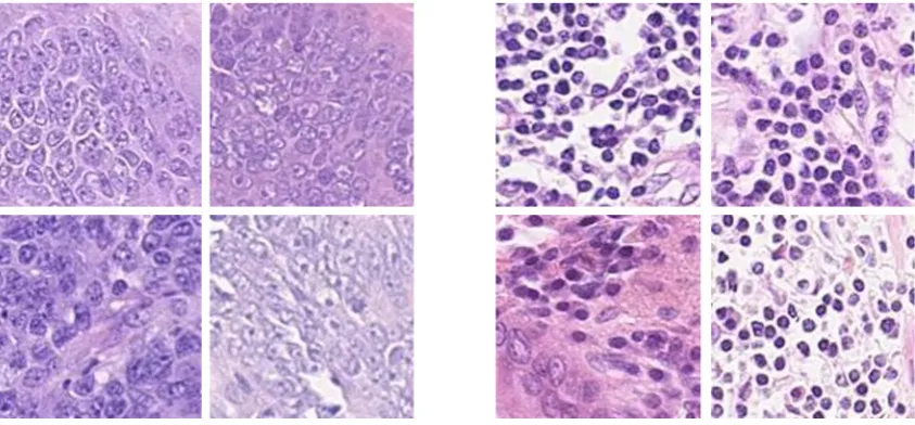
In tumor regions nuclei have different atypical characteristics, with non-uniform chromatin texture and irregularity in their shape and size. In tumor areas nuclei clump together, filling the inter-cellular regions, and the structure of individual nuclei becomes more difficult to discern. In contrast, nuclei remain relatively distinct in normal regions and maintain their structure and appearance (Fig 1). The arrangement of nuclear structures is a significant feature for tumor classification. In this paper, we propose a new approach to tumor segmentation in WSIs by characterizing the connectivity between cells, using persistent homology. Our approach works in the following ways : 1) a method for constructing persistent homology profiles based on topological features; 2) an algorithm for selection of exemplar patches from the training dataset based on highly activated nodes of a CNN; and 3) a variant ofk-NN classifier.

Fig. 1: (a) Tumor patches, exhibiting non-uniformity in chromatin texture and atypical characteristics. (b) Non-tumor patches showing the homo-geneous structure of normal nuclei.

2. Proposed Algorithm

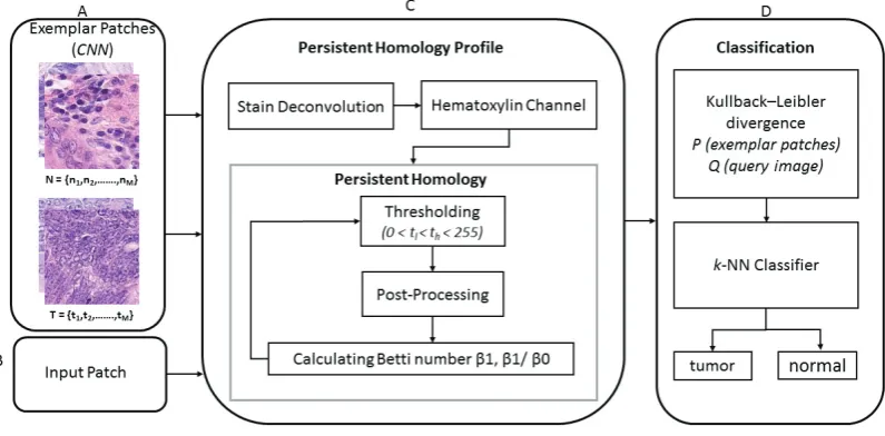
Given a colorectal WSI, we first divide it into patches. The problem is to then classify each patch as tumor or non-tumor. We approach this problem by exploring the connectivity between cells. We associate with each patch two statistical distributions, which we callpersistent homology profiles, computed using certain topological invariants, as will be explained below. For simplicity, we will explain our method using a single persistent homology profile for each patch. In that case, given two patches, we have the persistent homology profile for each, and the symmetrised Kullback-Leibler divergence (KLD) between these two distributions gives a numerical estimate for how far the patches are from each other. An input patchQis classified by ak-NN classifier, based on KLD distances between the persistent homology profiles of representative patches, denoted byP(Fig 2). We decide on our representative patches by training a CNN, and then selecting, separately for the tumor class and the non-tumor class, patches whose activation during the training is large. The essence of this approach is to use the subset of highly activated patches from convolutional layers as exemplars, rather than using the set of all the patches in the training dataset.

2.1. Persistent Homology

2.1.1. Overview.

Persistent homology is a fairly recent concept, surveyed in5_and6_{. LetMdenotes a graylevel image of sizemxn,} where gray intensities are integer values between 0 and 255 andBbe anm×nclosed rectangle. For each value of the thresholdt, letB(t)⊂Bbe the union of pixels with intensity less than or equal tot. We wantB(t) to be a closed subspace ofB, and so, with each pixel inB(t), we include its four corners and four sides. In effect, we binarize the intensity values inM, replacing any value less than or equal totby 0 and replacing other values by 1. The resulting matrixM(t) gives us a black and white image. The notation is supposed to remind us thatB(t) is the union of black pixels. We haveB(0) ⊆ B(1) ⊆ · · · ⊆ B(255) = B,so that Bis a filtered space, persistent homology’s essential ingredient. We will work with the zeroth_{Betti numberβ}

Fig. 2: (A) CNN based exemplar patches selected from the training dataset. (B) Input patch for testing. (C) Algorithm for persistent homology profiles. (D) Determine KLD between testing and exemplar patches and classify throughk-NN.

number of components ofB(t): this can be quickly computed from the matrixM. We are also interested in the first Betti numberβ1 : [0,255]∩Z→ Z, giving the number of independent circuits inB(t), or, equivalently, since we are working in the plane, the number of holes inB(t). To computeβ1(t), we first find the white components, that is the components of the complementW(t)= B\B(t) ofB(t). Astincreases, new components appear inB(t) and old components increase in size and amalgamate. Also, astincreases, and black pixels replace white pixels, black regions may coalesce to surround new white holes, or white holes may split into several white holes or disappear completely. Each of the two functionsβ0andβ1sometimes increases and sometimes decreases astvaries (see Fig 3), depending on the details of the image matrixM.

2.1.2. Persistent Homology Profiles (PHP)

A block diagram showing the computation of a persistent homology based profile is shown in Fig 2C. Histology images stained on different occasions often vary considerably in color. To overcome this problem, we first carry out stain normalization7_{to obtain consistency. For each thresholdt, we convert the normalized image into a binary image,} prior to computing persistent homology. In tumor regions, nuclei have atypical characteristics and lie relatively close to each other. Hence, homology classes do not show rapid changes while merging and forming into new classes. By contrast, normal regions have a high rate of change since cells are distinct and, when the threshold increases, the holes between them are filled rapidly. The derived profiles for tumor and non-tumor patches are distinguishable in terms of their qualitative characteristics (Fig 3).

2.2. Selection of Exemplars from CNN

The CNN used for extracting the exemplar patches for tumor and non-tumor regions is shown in Fig 4. The con-volutional layers contain the set of learnt features with a combination of extremely high and extremely low frequency information. We acquire the activation matrix after CL3 by performing ReLU and MP, which rectify the feature maps by ensuring the learnt features are always positive. For theith_{training patch, we obtain an activation matrix}

α(i) _∈RH×W×Z_{, whereH,W, andZdenote the size of the matrix in each dimension. For the architecture used in this} work,H=24,W=24, andZ=108. On the basis of the learnt features, we then calculate the mean activation value of thezth_{learnt filter response according to (1). Letα}(i)

hwzdenotes the (h,w,z) element ofα

122 Talha Qaiser et al. / Procedia Computer Science 90 ( 2016 ) 119 – 124

Threshold value

50 100 150 200 250

0 0.01 0.02

0.03 _Tumor

Non-tumor

(a)

Threshold value

100 150 200 250

0 0.02 0.04

0.06 _Tumor

Non-tumor

(b)

Fig. 3: Persistent homology profile for representative patches (a)β1and (b)β1/β0, showing median values with their first and third quartile, for tumor(red)and non-tumor(blue).

value of thezth_{filter response ofα}(i)_{is defined as}

α(i)

z =

1 H·W

h,w α(i)

h,w,z. (1)

For each filter responsezof the filter responses, we define

M(z)=argmaxi{α(zi)} (2)

whereiruns over all patches in the training set. ThenM(z) is a particularly important training patch, and we use it as an exemplar. The top six exemplar patches are shown in Fig 5.

Fig. 4: Our CNN architecture has 6 layers: 3 convolutional layers, 2 fully connected layers (not shown), and 1 classification layer (not shown). An input patch is of size 128×128. The first convolutional layer (CL1) convolves the input with 36 learnt (7×7)-filters. The resulting 36-feature maps of size 122×122 are then passed through a rectified linear unit (ReLU) and max pooling (MP) is then carried out, with stride 2 in each direction. The second convolutional layer (CL2) contains 72 learnt (6×6)-filters with ReLU and an MP layer of stride 2. The CL3 layer consists of 108 learnt (5×5)-filters with ReLU and an MP layer with stride 2. After CL3, we recorded the top activations from the activation matrix. The above architecture is inspired by8_.

2.3. Patch Classification

(a) (b) Fig. 5: The top 6 highly activated patches from the training dataset (a) tumor (b) non-tumor.

that of each exemplar patch (P). So, associated with each input patchQ, we have computed a list of distances to the exemplar patchesD(Q) = (dT1,dT2, . . . ,dTA,dN1,dN2, . . . ,dNB).Theknearest neighbors ofQare determined by choosing theksmallest distances in this list.

3. Experimental Results and Discussion

3.1. Dataset and Implementation Details

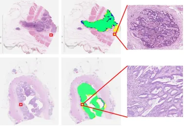
We collected 74 H&E stained WSIs of colorectal tumors. The tumor areas for this dataset were marked by an expert pathologist. The dataset was divided into 50 WSIs for training and 24 WSIs for testing. We randomly selected a total of 18944 (12824 training and 6120 testing) patches each of size 128×128 pixels with equal number of patches from both classes. The classification of tumor patches is fairly challenging due to the high degree of heterogeneity in tumor regions. As can be seen in Fig 6, our algorithm correctly segments the tumor region lying inside or on periphery of the hand marked tumor regions. Our expert pathologist marked the tumor regions only approximately, and so the regions marked in yellow in the “ground truth” annotations by the expert were not originally included. We chose 108 exemplar tumor patches and similarly 108 for non-tumor patches. Fork-NN, we selectedk=11 neighbors for classification and the value ofc(Q) was selected asc(Q)=0.2 maxd∈D(Q){d}. Our algorithm was implemented in Matlab using MatConvNet with Intel Xeon E5-2887W and GeForce GTX TitanX. Finally, the segmentation accuracy was measured by the F1 score (F1=2·Precision·Recall/(Precision+Recall)).

3.2. Results and Discussion

We compared our algorithm (PHP) with two state-of-the-art methods, including conventional CNN and HyMaP9_. For PHP, we used variant ofk-NN as a classifier (as described in Section 2.3). For CNN we used the same architecture as that described in Fig 4 with some modifications. After the convolution layers, we used two fully connected and one classification layer with the numbers of hidden neurons 512, 512, and 2, respectively. For HyMaP we used the original implementation9 _{based on a set of texture features and random projections with ensemble clustering.} One sees in Table 1 that PHP achieved significantly better classification accuracy than that of HyMaP9. PHP also achieved a slightly better precision and F1 score than conventional CNN. PHP also provided a reasonable balance between precision and recall, with the result that the number of false positives was roughly equal to the number of false negatives. Our method is computationally less expensive than either of the two currently standard techniques.

Table 1: Comparing PHP with existing state-of-the-art.

Method Precision Recall F1 Score

PHP 0.9492 0.957 0.9531

conventional CNN 0.911 0.988 0.9524

124 Talha Qaiser et al. / Procedia Computer Science 90 ( 2016 ) 119 – 124

Fig. 6: Here we show the result of applying persistent homology profiles (PHP) to tumor segmentation of two different WSIs: (Left) Input image. (Center)Green: PHP agrees with the original expert tumor annotation. Blue: regions marked as non-tumor by PHP, but as tumor by expert annotation.Yellow:regions marked as tumor by PHP, but as non-tumor by expert annotation. (Right) Zoom in showing that one of our supposedly “false-positive” regions, marked by PHP as tumor and originally annotated as non-tumor, is in fact tumor.

4. Conclusions

In this work, we introduced a tumor segmentation approach for histology WSIs based on persistent homology profiles. Here we explored the degree of connectivity between nuclei using and persistent homology. We found that the tumor and non-tumor patches have distinguishable homology profiles. Experimental results using a challenging dataset demonstrate the robustness and significance of persistent homology profiles, and PHP performed better on our test dataset than standard existing methods including conventional CNN. The resulting algorithm is an order of magnitude faster then the standard CNN.

References

1. Torre, L.A., Bray, F., Siegel, R.L., Ferlay, J., Lortet-Tieulent, J., Jemal, A.. Global cancer statistics, 2012. CA: a cancer journal for clinicians2015;65(2):87–108.

2. Akbar, S., Jordan, L., Thompson, A.M., McKenna, S.J.. Tumor localization in tissue microarrays using rotation invariant superpixel pyramids. In:Biomedical Imaging (ISBI), 2015 IEEE 12th International Symposium on. IEEE; 2015, p. 1292–1295.

3. Al-Kofahi, Y., Lassoued, W., Lee, W., Roysam, B.. Improved automatic detection and segmentation of cell nuclei in histopathology images. Biomedical Engineering, IEEE Transactions on2010;57(4):841–852.

4. Gurcan, M.N., Pan, T., Shimada, H., Saltz, J.. Image analysis for neuroblastoma classification: segmentation of cell nuclei. In:Engineering in Medicine and Biology Society, 2006. EMBS’06. 28th Annual International Conference of the IEEE. IEEE; 2006, p. 4844–4847.

5. Edelsbrunner, H., Harer, J.. Persistent homology—a survey.Contemporary mathematics2008;453:257–282. 6. Carlsson, G.. Topology and data.Bulletin of the American Mathematical Society2009;46(2):255–308.

7. Khan, A.M., Rajpoot, N., Treanor, D., Magee, D.. A nonlinear mapping approach to stain normalization in digital histopathology images using image-specific color deconvolution.Biomedical Engineering, IEEE Transactions on2014;61(6):1729–1738.

8. Krizhevsky, A., Sutskever, I., Hinton, G.E.. Imagenet classification with deep convolutional neural networks. In: Advances in neural information processing systems. 2012, p. 1097–1105.