University of Warwick institutional repository: http://go.warwick.ac.uk/wrap
This paper is made available online in accordance with
publisher policies. Please scroll down to view the document
itself. Please refer to the repository record for this item and our
policy information available from the repository home page for
further information.
To see the final version of this paper please visit the publisher’s website.
Access to the published version may require a subscription.
Author(s): Adnan Ali, Ellák Somfai, and Stefan Grosskinsky
Article Title: Reproduction-time statistics and segregation patterns in
growing populations
Year of publication: Forthcoming
Link to published article:
http://pre.aps.org/accepted/E/a2070R13Y4210700e87e3956479b55e0
25e8c9a9f
arXiv:1111.2992v1 [q-bio.PE] 13 Nov 2011
Adnan Ali,1 Stefan Grosskinsky,1, 2 and Ell´ak Somfai1, 3 1
Centre for Complexity Science, University of Warwick, Coventry CV4 7AL, United Kingdom
2
Mathematics Institute, University of Warwick, Coventry CV4 7AL, United Kingdom
3
Department of Physics, University of Warwick, Coventry CV4 7AL, United Kingdom (Dated: November 15, 2011)
Pattern formation in microbial colonies of competing strains under purely space-limited population growth has recently attracted considerable research interest. We show that the reproduction time statistics of individuals has a significant impact on the sectoring patterns. Generalizing the standard Eden growth model, we introduce a simple one-parameter family of reproduction time distributions indexed by the variation coefficient δ ∈ [0,1], which includes deterministic (δ = 0) and memory-less exponential distribution (δ= 1) as extreme cases. We present convincing numerical evidence and heuristic arguments that the generalized model is still in the KPZ universality class, and the changes in patterns are due to changing prefactors in the scaling relations, which we are able to predict quantitatively. At the example of S. cerevisiae, we show that our approach using the variation coefficient also works for more realistic reproduction time distributions.
PACS numbers: 87.18.Hf, 89.75.Da, 05.40.-a, 61.43.Hv
I. INTRODUCTION
Spatial competition is a common phenomenon in growth processes and can lead to interesting collective phenomena such as fractal geometries and pattern for-mation [1–3]. This is relevant in biological contexts such as range expansions of biological species [4, 5] or growth of cells or microorganisms, as well as in social contexts such as the dynamics of human settlements or urbaniza-tion [6]. These phenomena often exhibit universal fea-tures which do not depend on the details of the particu-lar application, and have been studied extensively in the physics literature [2, 3, 7–10].
Our main motivating example will be growth of mi-crobes in two dimensional geometries, for which recently there have been several quantitative studies. In general, the growth patterns in this area are influenced by many factors, such as size, shape and motility of the individual organism [11], as well as environmental conditions such as distribution of resources and geometric constraints [12, 13], which in turn influence the proliferation rate or motility of organisms [14]. We will focus on cases where active motion of the individuals can be neglected on the timescale of growth, which leads to static patterns and is also a relevant regime for range expansions. We further assume that there is no shortage of resources, and growth and competition of species is purely space limited and spatially homogeneous. This situation can be studied for microbial colonies grown under precisely controlled conditions on petri dish with hard agar and rich growth medium. Under these conditions one expects the colony to form compact Eden-type clusters [12], which has re-cently been shown for various species including S. cere-visiae, E. coli, B. subtilis and S. marcescens [14, 15].
The Eden model [16] has been introduced as a basic model for the growth of cell colonies. It has later been shown to be in the KPZ universality class [3, 7, 17, 18], which describes the scaling properties of a large generic
class of growth models. In recent detailed studies of E. coli and S. cervisiae [14, 15, 19, 20] quantitative evi-dence for the KPZ scaling of growth patterns has been identified. The models used in these studies ignored all microscopic details reproduction, such as anisotropy of cells [21], and could therefore not explain or predict dif-ferences observed for different species. Nevertheless, they provided a good reproduction of the basic features such as KPZ exponents, which is a clear indication that segrega-tion itself is an emergent phenomenon. Fig. 1 shows dif-ferences in growth patterns in a circular geometry taken from [15] for E. coli and S. cervisiae. For both species the microbial populations are made of two strains, which are identical except having different fluorescent labeling. Reproduction is asexual, and the fluorescent label car-ries over to the offspring. At the beginning of the ex-periments the strains are well mixed, but during growth rough sector shaped segregated regions develop. The qualitative emergence of these segregation patterns and connections to annihilating diffusions has been studied in [15, 19, 20, 22], ignoring all details specific for a particular species.
(a) (b)
FIG. 1: (Color online) Fluorescent images of colonies of (a) E. coli and (b) S. cerevisiae. The scaling properties of both patterns are believed to be in the KPZ universality class, and the differences are due to microscopic details of the mode of reproduction and shape of the micro-organisms. The images have been taken with permission from [15], copyrighted (2007) by the National Academy of Sciences, U.S.A.
To systematically study these temporal correlations, we introduce a generic one-parameter family of reproduc-tion times, explained in detail in Secreproduc-tion II. We establish that the growth clusters and competition interfaces still show the characteristic scaling within the KPZ univer-sality class, and the effect of the variation coefficient is present only in prefactors. We predict these effects quan-titatively and find good agreement with simulation data; these results are presented in Section III. More realistic reproduction time distributions with a higher number of parameters are considered in Section IV, where we show that to a good approximation the effects can be sum-marized in the variation coefficient and mapped quan-titatively onto our generic one-parameter family of re-production times. Therefore, our results are expected to hold quite generally for unimodal reproduction time dis-tributions, and the variation coefficient alone determines the leading order statistics of competition patterns.
II. THE MODEL
For regular reproduction times with small variation co-efficient the use of a regular lattice would lead to strong lattice effects that affect the shape of the growing clus-ter. To avoid these we use a more realistic Eden growth model in a continuous domain in R2 with individuals modelled as circular hard-core particles with diameter 1, since we want to study purely the effect of time cor-relations. This leads to generalized Eden clusters which are compact with an interface that is rough due to the stochastic growth dynamics.
Let B(t) denote the general index set of particles p
at time t, (xp, yp)∈ R2 is the position of the centre of
particle p, and sp ∈ {1,2} is its type. We write B(t) = B1(t)∪B2(t) as the union of the sets of particles of type
1 and 2. We also associate with each particle the time it tries to reproduce next, Tp>0. Initially,Tp are i.i.d.
random variables with distribution Fδ with parameter
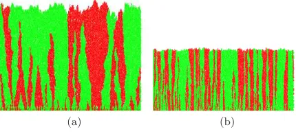
(a) (b)
FIG. 2: (Color online) A smaller variation coefficient δ in reproduction times (see (4) and (6)) leads to more regu-lar growth, smoother domain boundaries and finer sectors. Shown are simulated circular populations with (a)δ= 1 and (b)δ= 0.1. Both colonies have an initial radius of r0 = 50, and they are grown up to simulation timet= 50 leading to final radii of approximately 120 (a) and 95 (b).
δ∈[0,1], which is explained in detail below. After each reproduction Tp is incremented by a new waiting time
drawn from the same distribution. Note that we focus entirely on the neutral case, i.e. the reproduction time is independent of the type and both types have the same fitness. We describe the dynamics below in a recursive way.
Following a successful reproduction event of particlep
at timeTp, a new particle with indexq =|B(Tp−)|+ 1
is added with the same typesq =sp,
Bsp(Tp+) =Bsp(Tp−)∪ {q} (1)
HereB(T−) andB(T+) denote the index set just before and just after timeT. The position of the new particle is given by
(xq, yq) = (xp, yp) + (cosφ,sinφ), (2)
where φ ∈ [0,2π) is drawn uniformly at random. This is subject to a hard-core exclusion condition for circular particles, i.e. the euclidean distance to all other particle centres has to be at least 1, as well as to other constraints depending on the simulated geometry as explained be-low. Note that in our model the daughter cell touches its mother, which is often realistic but in fact not essen-tial, and the distance could also vary stochastically over a small range. The new reproduction times of mother and daughter are set as
Tp7→Tpold+T , Tq=Tpold+T′ , (3)
where T, T′ are i.i.d. reproduction time intervals with
distributionFδ. There can be variations on this where
mother and daughter have different reproduction times, which are discussed in Section IV. The next reproduc-tion event will then be attempted att = min
[image:3.595.64.289.50.151.2] [image:3.595.340.533.57.175.2]there is no available space for the offspring due to block-age by other particles. In this case the attempt is aban-doned andTp is set to∞, as due to the immobile nature
of the model this particle will never be able to reproduce. The initial conditions for spatial coordinates and types depend on the situation that is modelled. In this paper we mostly focus on an upward growth in a strip of length
Lwith periodic boundary conditions on the sides, where we take B(0) ={1, . . . , L} with (xp, yp) = (p,0), for all p∈B(0). The initial distribution of types can be either regular or random depending on whether we study single or interacting boundaries, and will be specified later.
In Section III for our main results we use reproduction times
T ∼1−δ+ Exp(1/δ), δ∈(0,1], (4)
i.e. T has exponential distribution with a time lag 1−
δ ∈ [0,1) and with mean fixed to hTi = 1 for all δ. The corresponding cumulative distribution function Fδ
is given by
Fδ(t) =
0 , t≤1−δ
1−e−(t−1+δ)/δ , t≥1−δ . (5)
The variation coefficient of this distribution is given by the standard deviation divided by the mean, which turns out to be just
p
hT2i − hTi2
hTi =
δ
1 =δ . (6)
With this family we can therefore study reproduction which is more regular then exponential with a fixed av-erage growth rate of unity (equivalent of setting the unit of time).
For δ = 1 this is a standard Eden cluster, but δ <1 introduces time correlations. While the correlations af-fect the fluctuations, we present convincing evidence that they decay fast enough not to change the fluctuation ex-ponents, so the system remains in the KPZ universality class. Furthermore we make quantitative predictions on theδ-dependence of non-universal parameters and com-pare them to simulations. The more synchronized growth leads to effects similar to the ones seen in experiments (Fig. 1). To give a visual impression of the patterns produced by the model, we show in Fig. 2 two growth patterns with δ = 1 and 0.1. The initial condition is a circle, and the types are distributed uniformly at random. The patterns are qualitatively similar to the experimen-tal ones in Fig. 1, and more regular growth leads to a finer sector structure. The same effect is shown on Fig. 3 for the simulations in a linear geometry with periodic boundary conditions, which is analyzed quantitatively in the next Section. Smaller values of δ also lead to more compact growth and smaller height values reached in the same time.
(a) (b)
FIG. 3: (Color online) Populations in a linear geometry with periodic boundary conditions in lateral direction with (a)δ= 1 and (b)δ= 0.1. Both populations have lateral widthL= 300, and the colonies are grown to a simulation timet≈50, leading to heights of approximately 70 (a) and 40 (b).
III. MAIN RESULTS
A. Quantitative analysis of the colony surface
In this Section we provide a detailed quantitative anal-ysis of the δ family of models in linear geometry with periodic boundary conditions (see Fig. 3), starting with the dynamical scaling properties of the growth interface. We regularize the surface to be able to define it as a function of the lateral coordinatexand timet as
y(x, t) := max
yp:p∈B(t),|xp−x| ≤1 . (7)
In case of overhangs (which are very rare) we take the largest possible height, and due to the discrete nature of our model this leads to a piecewise constant function.
The surface of a standard Eden growth cluster is known to be in the KPZ universality class [16, 18], i.e. a suitable scaling limit ofy(x, t) with vanishing particle diameter fulfills the KPZ equation
∂ty(x, t) =v0+ν∆y(x, t) +λ
2(∇y(x, t))
2+√Dη(x, t).
(8) Herev0, of the order of unity, corresponds to the growth
rate of the initial flat surface (related to the mean repro-duction rate and some geometrical effects), the surface tension term with ν > 0 represents surface relaxation, and the nonlinear term represents the lowest order con-tribution to lateral growth [18]. The fluctuations due to stochastic growth are described by space-time white noiseη(x, t), which is a mean 0 Gaussian process with correlations
η(x, t)η(x′, t′)
=δ(x−x′)δ(t−t′). (9)
We denote the average surface height by
h(t) := 1
L
Z L
0
y(x, t)dx , (10)
[image:4.595.330.545.58.157.2]10−5 10−4 10−3 10−2 10−1 10−2
10−1
t/Lz
S(t)/L
α
δ=1 δ=0.8 δ=0.6 δ=0.4 δ=0.2
FIG. 4: (Color online) Family-Vicsek scaling (12) of the sur-face roughnessS(t). The data collapse under rescaling with
α = 1/2 and z = 3/2 occurs in a scaling window which is narrower for smallδ due to intrinsic correlations. The differ-ent symbols correspond to differdiffer-ent values ofδ, and the color represents system size,L= 1500 (blue) andL= 4000 (red). The dashed lines indicate the expected slope β= 1/3. The data for L= 1500 has been averaged over 100 samples and forL= 4000 over 30 samples. The error bars are comparable to the size of the symbols.
has a proxy for time. Theδ-dependence of the average growth velocity of height as seen in Fig. 3 does not lead to leading order contributions to the statistical properties of the surface or the structure of sectoring patterns.
The roughness of the surface is given by the root mean squared displacement of the surface height as a function oft[3, 10], defined as
S(t) =D1
L
Z L
0
y(x, t)−h(t)2
dxE1/2 . (11)
The main properties of the surface y(x, t) can then be characterized by the Family-Vicsek scaling relation of the roughness
S(t) =Lαf(t/Lz), (12)
where the scaling functionf(u) has the property
f(u)∝
uβ u≪1
1 u≫1 . (13)
Such a scaling behaviour has been shown for many dis-crete models including ballistic deposition and continuum growth [3, 10, 18, 26, 27], and holds also for other uni-versality classes such as Edward Wilkinson. For the KPZ class in 1+1 dimensions the saturated interface roughness exponent is α= 1/2, the growth exponent is β = 1/3, and the dynamic exponent isz=α/β= 3/2.
Fig. 4 shows a data collapse for the roughnessS(t) for two system sizes, and for a number of different values of δ. As δ gets smaller, the surface becomes less rough
101 102 103 100
101
l
C(l,t)
δ=1 δ=0.8 δ=0.6 δ=0.4 δ=0.2
FIG. 5: (Color online) The height-height correlation function
C(l, t) forL= 4000 att= 11000 for various values ofδ. The data has been averaged over 30 samples, and the error bars are comparable to the size of the symbols. The dashed lines indicate the expected slope 1/2.
due to a more synchronized growth. The dashed lines indicate the power law growth with exponentβ= 1/3 in the scaling window. This window ends aroundt/Lz≈1
due to finite size effects, where the lateral correlation length reaches the system size and the surface fluctua-tions saturate. For smalltthe system exhibits a transient behaviour before entering the KPZ scaling due to local correlations resulting from the non-zero particle size and stochastic growth rules. As we quantify later, these cor-relations are much higher for more synchronized growth at small δ, which leads to a significant increase in the transient regime. The transient time scale is indepen-dent of system size and vanishes in the scaling limit, so that the length of the KPZ scaling window increases with
L. This behaviour can be observed in Fig. 4 where for the smallest valueδ= 0.2 the scaling regime is still hard to identify for the accessible system sizes.
Another characteristic quantity is the height-height correlation function defined as [3, 28, 29]
C(l, t) =D1
L
Z L
0
(y(x, t)−y(x+l, t))2dxE1/2. (14)
For a KPZ surface in 1 + 1 dimensions this obeys the scaling behaviour
C(l, t)∼
(
(2Dνl)1/2 l≪ξ
k(t) D
2ν
2/3
(λt)1/3 l≫ξ
k(t)
, (15)
whereξk(t) is defined to be the lateral correlation length scale and takes the form [3, 29, 30]
[image:5.595.337.530.60.219.2] [image:5.595.71.268.61.216.2]0.2 0.3 0.4 0.5 0.6 0.7 0.8 0.9 1 0.1
0.2 0.3 0.4 0.5 0.6 0.7 0.8 0.9 1
δ
D/2
ν
Data 0.5299(δ2
+0.4194)2
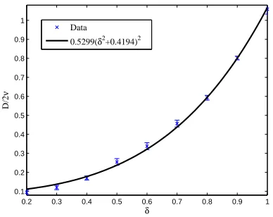
FIG. 6: (Color online) Dependence of the KPZ parameters
D/(2ν) onδ. Data are obtained from (15) by fitting the pref-actor of the power law in Fig. 5, using that the proportionality constant is very close to 1 (cf. derivation (B11) in the Ap-pendix). The data are in good agreement with the prediction (21) with fitted parametersǫ≈0.42 andD/(2ν)(δ= 1)≈1.1.
withl, and whenl exceeds the lateral correlation length
ξk(t) it reaches a value that depends on the timetand the parameters of (8). This is shown in Fig. 5, whereC(l, t) is plotted for various values ofδ, and the data agree well with the exponent α= 1/2 for the KPZ class indicated by dashed lines.
The time correlations introduced by the partial syn-chronization can be estimated by considering a chain of
N growth events where each particle is the direct de-scendant of the previous one. Each added particle corre-sponds to a height change ∆yi, and has an associated
waiting time Ti with distribution (4). During time t
there are N(t) growth events, and since the average re-production time is 1 with varianceδ2, we havehN(t)i ≈t
and var(N(t)) ≈δ2t. The height of the last particle is
yN(t)=P N(t)
i ∆yi, leading to
var(yN(t)) =h∆yii2var(N(t)) +hN(t)ivar(∆yi). (17)
The terms in this expression correspond to two sources of uncertainty: (i) due to the randomness inTi the
num-ber of growth events vary with var(N(t)), and (ii) the individual height increments are random with var(∆yi).
This leads to
var(yN(t))≈th∆yii2(δ2+ǫ2), (18)
whereǫ=p
var(∆yi)/h∆yiidenotes the variation
coeffi-cient of the height fluctuations due to geometric effects. We define the correlation timeτas the amount of time by which the uncertainty of the height of the chain be-comes comparable to one particle diameter, var(yN(τ)) =
O(1). Since h∆yii is largely independent of δ (cf.
Ap-pendix A), the time correlation induces a fixed intrinsic
vertical correlation length
τ∼ δ2+1 ǫ2 (19)
in the model. This correlation length reduces fluctuations and leads to an increase in the saturation time tsat of
the system, namelytsat/τ ∼ Lz, a modification of the
usual relation with the system sizeL. Analogous to the standard derivation of the time-dependence of the lateral correlation length [3], this leads to
ξk(t)∼(t/τ)1/z . (20)
Together with (16) from the behaviour of the correlation length, we expect
D/(2ν)∼(δ2+ǫ2)2, (21)
sinceλ turns out to be largely independent of δ. This is shown to be in very good agreement with the data in Fig. 6, for fitted values of ǫand a prefactor. The fit value for ǫ and the ratio D/(2ν) for δ = 1 (the usual Eden model) are compatible with simple theoretical ar-guments (see Appendix A). So the very basic argument above to derive an intrinsic vertical correlation length explains theδ-dependence of the surface properties very well. Measuring height in this intrinsic length scale, we observe a standard KPZ behaviour with critical expo-nents being unchanged, since the intrinsic correlations are short range (i.e. decay exponentially on the scaleτ). This is in contrast to effects of long-range correlations where the exponents typically change, see e.g. studies with long-range temporally correlated noise [31–33] or memory and delay effects using fractional time deriva-tives and integral/delay equations [34–36].
B. Domain boundaries
In this section we derive the superdiffusive behaviour of the domain boundaries between the species from the scaling properties of the interface. Since the boundaries grow locally perpendicular to the rough surface, they are expected to be superdiffusive with Hurst exponent 2/3, which has been shown for a solid on solid growth model in [37] and has been observed in [15] for experimental data. In order to confirm this quantitatively for our model, we perform simulations with initial conditionsB1(0) =
{1, . . . ,[L/2]} and B2(0) = {[L/2] + 1, . . . , L}, i.e. the
initial types are all red on the left half and all green on the right half of the linear system. Therefore we have two sector boundariesX1 and X2 with initial positions
X1(0) = 1/2 and X2(0) = [L/2] + 1/2. After growing
the whole cluster, we define the boundary as a function of height via the leftmost particle in a strip of width 2 and medium heighth:
X1(h) = minxp+ 1/2 :|yp−h|<1, p∈B1
[image:6.595.76.270.61.215.2]101 102 103 100
101 102 103 104
h
M(h)/
σδ
2
δ=1 δ=0.8 δ=0.6 δ=0.4 δ=0.2 h4/3
(a)
0.2 0.3 0.4 0.5 0.6 0.7 0.8 0.9 1 0.1
0.15 0.2 0.25 0.3 0.35 0.4
δ
σ
2 δ
Data 0.2765(δ2
+0.3958)4/3
(b)
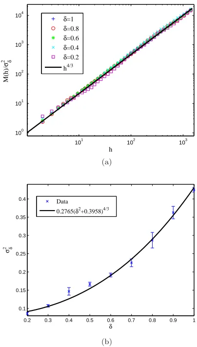
FIG. 7: (Color online) Scaling behaviour of the mean square displacement M(h) (24). The system size is L = 1000 and the data is averaged over 500 samples and the error bars are comparable to the size of the symbols. (a) Data collapse of the normalized quantityM(h)/σ2
δ as a function of height h for several values ofδ. The values in the normalizationσ2
δare
taken from the best fit shown as full line in (b). Each curve follows a power law with exponent 4/3, the line corresponding toh4/3
is shown as comparison. (b) The prefactorσ2 δ, where the data are best fits according to (24). The full line used for the collapse in (a) follows the prediction (δ2
+ǫ2 )4/3
with fittedǫ= 0.40, which is compatible with the fit in Fig. 6.
where we take the periodic boundary conditions into ac-count. The simulations are performed on a system of size
L= 1000, and run until a time oft= 2000, which is well before the expected time of annihilation, which is of or-derL3/2proportional to the saturation timescale in the
KPZ class. Therefore we can treat the sector boundaries as two independent realizations of the boundary process
X(h) :h≥0
.
As has been noted already in [37], this process is ex-pected to follow the same scaling as the lateral correlation
length. For the mean square displacement
M(h) :=D X(h)−X(0)2E
(23)
we therefore get with (16) and (21), using the linear re-lationship betweenhandt,
M(h)≈σδ2h4/3∼ξ2k(h) (24)
whereσ2
δ ∝(δ2+ǫ2)4/3. This prediction is in very good
agreement with data for the scaling ofM(h) and its pref-actor as presented in Fig. 7, and the fit value for ǫ2 is
consistent with the one in Fig. 6. As before, forD/(2ν) theδ-dependence is absorbed by the prefactor, and the power law exponent 4/3 for M(h) remains unchanged from standard KPZ behaviour studied also in [37].
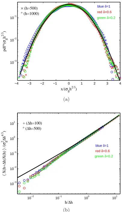
We can further investigate the law of the process
X(h) :h≥0
. The data presented in Fig. 8(a) clearly support that X(h) is a Gaussian process. A fractional Brownian motion with stationary increments seems to be a natural model for the X(h) in the KPZ scaling window. This is confirmed by the behaviour of the cor-relation function hX(h+ ∆h)X(h)i, which is shown in Fig. 8(b) for variousδand two values of the lag ∆h >0. For a fractional Brownian motion with mean square dis-placement (24) we expect
X(h+∆h)X(h)
≈ σ
2 δ
2 (h+∆h)
4/3+h4/3
−|∆h|4/3
(25) for all ∆h > 0 and h > 0 sufficiently large to have no effects from the flat initial condition. For simplicity we have assumed here thatX(0) = 0.
This is in good agreement with the data, and we con-clude that the sector boundaries can be modeled by frac-tional Brownian motions with superdiffusive Hurst expo-nent 2/3 and aδ-dependent prefactorσδ (24).
C. Sector patterns
In [19], and also [20, 22] under the assumption of diffu-sive scaling, it was shown how the understanding of the single boundary dynamics leads to a prediction for sector statistics for well-mixed initial conditions. In this section we shortly review this approach and show that it carries over straight away to systems with δ < 1. The sector boundariesXi(h) interact by diffusion limited
annihila-tion which drives a coarsening process, as can be seen in Fig. 3 for two linear populations with different values of
δ. Both systems have the same initial condition with a flat line of particles of independently chosen types, and the finer coarsening patterns for smaller values ofδ re-sult from the reduced boundary fluctuations due to the prefactorσδ (24).
LetN(h) be the number of sector boundaries at height
[image:7.595.67.269.60.416.2]−4 −3 −2 −1 0 1 2 3 4 10−3
10−2 10−1
x/(σδh2/3)
pdf*(
σδ
h
2/3
)
blue δ=1 red δ=0.6
green δ=0.2 × (h=500)
° (h=1000)
(a)
10−2 10−1 100 101 10−3
10−2 10−1 100 101
h/∆h
〈
X(h+
∆
h)X(h)
〉
/(
σ δ
2∆
h
4/3
)
blue δ=1 red δ=0.6
green δ=0.2 + (∆h=100)
° (∆h=500)
(b)
FIG. 8: (Color online) The sector boundaryX(h) behaves like a fractional Brownian motion. (a) The standardized prob-ability density function (pdf) of X(h) as a function of the rescaled argumentx/(σδh2/3) for different heightshand val-ues of δ. The black solid parabola is the pdf of a standard Gaussian on a logarithmic scale. (b) The covariance function
X(h+ ∆h)X(h)
shows the behaviour (25), which is plotted as the solid black curve. After rescaling we get a data collapse as a function ofh/∆h, which agrees well with the prediction ifhis sufficiently large and the flat boundary conditions be-come irrelevant. Data are averages over 1000 realizations and the error bars are comparable to the size of the symbols.
proportional to the root mean square displacement, and decays according to
hN(h)i ≈p 1
4πM(h) ∼ 1
σδ
h−2/3 . (26)
This prediction is confirmed in Fig. 9, where we plot hN(h)ifor variousδ, and obtain a data collapse by mul-tiplying the data with p
4πσ2
δ/L, [39]. We include the
system sizeLin the rescaling so that rescaled quantities are of order 1, and all data collapse on the functionh−2/3
without prefactor.
101 102 103 104 10−2
10−1
h
〈
N(h)
〉
/(L/(4
πσδ
2)
1/2
)
δ=1 δ=0.8 δ=0.6 δ=0.4 δ=0.2 h−2/3
FIG. 9: (Color online) The average number of sector bound-aries hN(h)i follow a power law (26) with exponent −2/3, which is indicated by the full line. The data are plotted for a system sizeL= 1500 and various values ofδ(see legend), and collapse on the function h−2/3 when rescaled by L/p4πσ2
δ.
Data are averages over 500 realizations and the error bars are comparable to the size of the symbols.
Using (26), we can predict the expected number of sector boundaries at the final height in the simulations shown in Figure 3. Forδ= 1, the final height is h≈70 leading to hN(h)i ≈ 7.6, and for δ = 0.1, h≈ 40 with hN(h)i ≈ 32. These numbers are compatible with the simulation samples shown which have 6 and 34 sector boundaries remaining, respectively.
In general, diffusion limited annihilation is very well understood, and there are exact formulas also for higher order correlation functions [40], which can be derived from the behaviour of a single boundary (24). This demonstrates that the behaviour of populations is funda-mentally the same for all values ofδand characterized by the KPZ universality class, and the observed difference in coarsening patterns can be explained by the functional behaviour of the prefactors.
IV. REALISTIC REPRODUCTION TIMES
[image:8.595.329.532.60.217.2] [image:8.595.66.269.61.414.2]im-Tr
Tm+Tr
TH∆=0.356L
TH∆=0.244L
0.0 0.5 1.0 1.5 2.0
0.0 0.5 1.0 1.5 2.0 2.5
tXT\
(a)
0.2 0.25 0.3 0.35 0.4 0.45 0.5 0.55 0.6 0.08
0.1 0.12 0.14 0.16 0.18 0.2
δ
σδ
2
δ−family M D M and D
(b)
FIG. 10: (Color online) Comparison of realistic reproduction times with theδmodel. (a) The probability density functions of reproduction times of mother cells Tr (full red line) and daughter cellsTm+Tr(dashed red line) with normalized mean compared toT from (4) with correspondingδ(blue). (b) The prefactor of the mean squared displacementσ2
δ as introduced in (24) and Fig. 7. The data correspond to reproduction times
Tr for all cells (denoted M),Tm+Tr for all cells (denoted D) and the most realistic mixed model (denoted M and D) as explained in the text. All these cases are consistent with previous results from Fig. 7.
mediately restart this reproduction process, whereas the daughter cell has to grow to a certain size in order to be classed as a mother and to be able to reproduce. We denote this time to maturity byTmand the reproduction
time of (mother) cells byTr.
The results in [23–25] suggest that Gamma distribu-tions are a reasonable fit for the statistics forTmandTr,
where
Tr∼ρ0+ Gamma(ρ1, ρ2), (27)
with delay ρ0 > 0. The parameters ρ1, ρ2 denote the
shape and scale of the Gamma distribution, which has a probability density function
fρ1,ρ2(t) =t
ρ1−1exp (−t/ρ2)
Γ(ρ1)ρρ21
, t≥0 .
The time to maturity is distributed as
Tm∼Gamma(ρ3, ρ4), (28)
and in [25] data are presented for which the parameters can be fitted toρ0≈1.0,ρ1≈1.7,ρ2≈0.51,ρ3≈9 and
ρ4≈0.3. The unit ofρ0, ρ2 andρ4are hours andρ1,ρ3
are dimensionless numbers.
The random variablesTmandTrmay be assumed to be
independent and the time until a newly born daughter cell can reproduce is distributed as the sumTm+Tr. Note
that the expected value of reproduction times hTri = ρ0+ρ1ρ2= 1.86 is smaller than that for times to maturity
hTmi = ρ3ρ4 = 2.52 but of the same order. The real
time scale for these numbers is hours, but we are only interested in the shape of these distributions rescaled to mean 1 like our previous model.
The distribution (4) ofδ-dependent reproduction times can be written asT ∼1−δ+ Gamma(1, δ), since expo-nentials are a particular case of Gamma random vari-ables with shape parameter 1. The reproduction time
Tr of mother andTm+Trof daughter cells are also
uni-modal with a delay, and very similar in shape to T in our model. This can be seen in Fig. 10(a), where we plot the probability densities renormalized to mean 1. Analogous to (6), we can compute the variation coeffi-cients ofTr and (Tm+Tr), which turn out to be 0.356
and 0.244, respectively. To confirm that the behaviour of sector boundaries can be well predicted by the varia-tion coefficient, we present data of three simulavaria-tions in Fig. 10(b): one with reproduction times Tr for mother
and Td+Tr for daughter cells as explained above, one
withTr for all cells, and one with Tr+Tmfor all cells.
The mean squared displacementM(h) for these models also shows a power law with exponent 4/3 analogous to Fig. 7, and the prefactorsσδ match well with our
simpli-fied model.
To estimate the variation coefficient in the model with mother and daughter cells, we measure the fraction of reproduction events of daughter cells to be pd = 0.88,
andpm= 0.12 for mother cells. The reproduction time
of the union of mother and daughter cells is then taken as
T = Θ(Tm+Tr) + (1−Θ)Tr , (29)
where the independent Bernoulli variable Θ∼Be(pd)∈
{0,1} indicates reproduction of a daughter. The varia-tion coefficient ofT turns out to be 0.322. In all three combinations of realistic reproduction times we find that the generic family ofFδ introduced in (4) provides a good
[image:9.595.72.274.46.378.2]V. CONCLUSION
We have introduced a generic generalization of the Eden growth model with competing species, regarding the reproduction time statistics of the individuals. This is highly relevant in biological growth phenomena, and can have significant influence on the sectoring patterns observed e.g. in microbial colonies. Although microbial species growth is the prime example, our results also ap-ply to more general phenomena of space limited growth with inheritance, where the entities have a complex inter-nal structure that leads to non-exponential reproduction times, such as colonization/range expansions or epidemic spreading of different virus strands. Our main result is that, as long as the reproduction time statistics have fi-nite variation coefficients, the induced correlations are lo-cal and the macroscopic behaviour of the system is well described by the KPZ universality class. The dependence of the relevant parameters in that macroscopic descrip-tion on the variadescrip-tion coefficient (a microscopic property of the system) is well understood by simple heuristic ar-guments, which we support with detailed numerical evi-dence.
The results in this paper can be used for quantitative predictions of sectoring patterns for species of approx-imately isotropic shape, such as S. cerevisiae. It is an interesting question if the simple mechanism of time cor-relations due to reproduction time statistics with variable variation coefficients is enough to quantitatively explain sectoring patterns in real experiments, which is currently under investigation. It could well be that other fac-tors influencing e.g. the choice of growth direction have to be included, to account for an effective attraction of cells which is often observed in the growth of microbial colonies. Such an effect would further smoothen the sur-face and the fluctuations of sector boundaries. In this paper we have focused on purely temporal correlations, but it should also be possible to describe spatial effects due non-isotropic particle shapes with the same methods.
Acknowledgments
The authors thank O. Hallatschek for useful discus-sions. This work was supported by the Engineering and Physical Sciences Research Council (EPSRC), grant no. EP/E501311/1.
Appendix A: Effect of geometric disorder
The squared variation coefficientǫ2 in (19) due to
ge-ometric disorder has been consistently fitted to values around 0.4 with our data in Section III. This value is compatible with the following very simple argument. Consider a single growth event around an isolated spher-ical particle with diameter 1, with direction α chosen uniformly in a cone with opening angle π/2 around the
vertical axis. This leads toh∆yii=R π/2
−π/2cosα dα
π ≈0.64
and
ǫ2≈
Z π/2
−π/2
cos2αdα
π − h∆yii
2.
h∆yii2≈0.23, (A1)
which is of the same order as the fitted values. Choosing only a slightly larger opening angle 0.55π of the cone leads toǫ2 ≈0.39 and h∆y
ii ≈ 0.57. These are in good
agreement with the fitted values and with measurements ofh∆yii(not shown). The latter show some dependence
onδ, related also to the compactness of growth as seen in Figs. 2 and 3, but this does not contribute to our results on a significant level so we ignore this dependence. Actual growth events in the simulation are of course often obstructed by neighbouring particles, but the right order of magnitude of the parameters can be explained by the basic argument above.
Appendix B: Deriving the correlation functionC(l, t)
We use the mode coupling method [29], in order to find an exact analytical expression of the correlation function Eq. (14) as shown in Eq. (15). The idea of the mode coupling approximation is that properties of solutions of the KPZ equation (8) may be derived by first considering the linear Edwards-Wilkinson equation [41] for λ = 0. We further consider the co-moving frame, so thatv0= 0,
and the equation then reads
∂ty(x, t) =ν∆y(x, t) +
√
Dη(x, t). (B1)
We denote by
ˆ
y(k, t) =
Z ∞
−∞
dx y(x, t)e−ikx
the Fourier transform of the functiony(x, t). The evolu-tion of the funcevolu-tion ˆy(k, t) satisfies
∂tyˆ(k, t) =−νk2yˆ(k, t) +
√
Dηˆ(k, t). (B2) Here ˆη(k, t) is the spatial Fourier transform of the white noiseη(x, t), where ˆη(k, t) has a mean 0 with correlations
ˆ
η(k, t)ˆη(k′, t′)
= 1
2πδ(k+k
′)δ(t−t′). (B3)
A formal solution of (B2) can be obtained, and after in-verse Fourier transform this leads to
y(x, t) =√D
Z ∞
−∞ dk eikx
Z t
0
dsηˆ(k, s)e−νk2(t−s) . (B4)
The correlation function C(l, t) defined in (14) can be represented as
C(l, t)2= 2
Z L
0
dx
y(x, t)2−y(l+x, t)y(x, t)
Using the solution (B4) we can compute
Z L
0
dx
y(l+x, t)y(x, t)
= D 2νπ
Z ∞
0
dkcos(kl) k2 [1−e−
2νk2
t] ,
(B6) where we have used that the Fourier transform is even in k. Taken together, this leads to an expression for the correlation function (14) of the Edwards-Wilkinson equation
C(l, t)2= D
νπ
Z ∞
0
dk k−2 1−cos(kl)
[1−e−2νk2
t]. (B7)
In order to compute the correlation function for the KPZ equation (8) we substitute length scale dependent parametersD(k) andν(k) into (B7), which are obtained from the renormalization group flow equations [3, 18, 29]. Ind= 2 dimensions these are given by
ν(k) = ν1[(1−αB) +αB/k]1/2 ,
D(k) = D1[(1−αB) +αB/k]1/2 , (B8)
andλ(k) =λ1, where
αB=
λ2 1D1
4π2ν3 1
.
Here (λ1, ν1, D1) are the parameters fork= 1 where no
renormalization has taken place. Plugging this into (B7) and only considering the most dominant terms, we obtain
C(l, t)2= D1
ν1π
Z ∞
0
dk k−2 1−cos(kl)
[1−e−Bk3/2t],
(B9)
whereB= 2ν1α1B/2= √
2 π λ
p
D1/2ν1 .
If we taket→ ∞in Eq. (B9) we get
C(l, t)2→ D1
ν1π
Z ∞
0
dk k−2 1−cos(kl)
= D1 2ν1
l .(B10)
With (B8)D/ν =D1/ν1 is independent of the scale k,
and thus
C(l, t)≈D 2νl
1/2
for l≪ξk(t). (B11)
For finite time, numerical integration of (B9) in the large
llimit gives
lim
l→∞C(l, t)
2
≈2.7 D
νπ(Bt)
2/3.
Together with (B11) and the definition (14) of the corre-lation length this leads to
lim
l→∞C(l, t)≈
5.4×21/3D
2ν
4/3
π−5/3(λt)2/31/2 ,
(B12) and
ξk(t)≈5.4×21/3D 2ν
1/3
π−5/3(λt)2/3 . (B13)
[1] A. M. Lacasta, I. R. Cantalapiedra, C. E. Auguet, A. Pe˜naranda, and L. Ram´ırez-Piscina, Phys. Rev. E59, 7036 (1999).
[2] M. Matsushita, J. Wakita, H. Itoh, K. Watanabe, T. Arai, T. Matsuyama, H. Sakaguchi, and M. Mimura, Physica A274, 190 (1999).
[3] A.-L. Barabasi and H. E. Stanley, Fractal concepts in surface growth (Cambridge University Press, 1995), 1st ed.
[4] D. Wegmann, M. Currat, and L. Excoffier, Genetics174
(2006).
[5] M. C. Fisher, G. L. Koenig, T. J. White, G. San-Blas, R. Negroni, I. G. Alvarez, B. Wanke, and J. W. Taylor, PNAS98, 4558 (2001).
[6] C. Finlayson, TREE20, 457 (2005).
[7] T. Vicsek, M. Cserz˝o, and V. K. Horv´ath, Physica A167, 315 (1990).
[8] D. Avnir,The Fractal Approach to Heterogeneous Chem-istry(Wiley-Blackwell, 1989).
[9] E. Ben-Jacob and P. Garik, Nature343, 523 (1990). [10] P. Meakin,Fractals, Scaling and Growth Far from
Equi-librium(Cambridge University Press, 1998), 1st ed. [11] J. Wakita, H. Itoh, T. Matsuyama, and M. Matsushita,
J. Phys. Soc. Jpn.66, 67 (1997).
[12] M. Ohgiwari, M. Matsushita, and T. Matsuyama, J. Phys. Soc. Jpn.61, 816 (1992).
[13] D. W. Thompson,On growth and form (Cambridge Uni-versity Press, 1992), 1st ed.
[14] R. Tokita, T. Katoh, Y. Maeda, J. Wakita, M. Sano, T. Matsuyama, and M. Matsushita, J. Phys. Soc. Jpn.
78, 074005 (2009).
[15] O. Hallatschek, P. Hersen, S. Ramanathan, and D. R. Nelson, PNAS104, 19926 (2007).
[16] M. Eden, Proc. Fourth Berkeley Symposium on Math Statistics and Probility.4, 223 (1961).
[17] T. Vicsek,Fractal Growth Phenomena (World Scientific Publishing, 1991), 2nd ed.
[18] M. Kardar, G. Parisi, and Y.-C. Zhang, Phys. Rev. Lett.
56, 889 (1986).
[19] A. Ali and S. Grosskinsky, ACS13, 349 (2010).
[20] O. Hallatschek and D. R. Nelson, Evolution 64, 193 (2010).
[21] B. D. Slaughter, S. E. Smith, and R. Li, CSH2(2009). [22] K. S. Korolev, M. Avlund, O. Hallatschek, and D. R.
Nelson, Rev. Mod. Phys.82, 1691 (2010).
and M. F. Tuite, Math. Med. Biol21, 369 (2004). [24] D. J. Cole, B. J. T. Morgan, M. S. Ridout, L. J. Byrne,
and M. F. Tuite, Biometrics63, 1023 (2007).
[25] K. J. Palmer, M. S. Ridout, and B. J. T. Morgan, J. Roy. Statist. Soc. Ser. C Appl. Statist.57, 379 (2008). [26] M. A. C. Huergo, M. A. Pasquale, A. E. Bolz´an, A. J.
Arvia, and P. H. Gonz´alez, Phys. Rev. E 82, 031903 (2010).
[27] F. Family and T. Vicsek, J. Phys. A.18(1985). [28] J. Krug, P. Meakin, and T. Halpin-Healy, Phys. Rev. A.
45, 638 (1992).
[29] J. G. Amar and F. Family, Phys. Rev. A.45, 5378 (1992). [30] M. Rost and J. Krug, Physica D88, 1 (1995).
[31] E. Medina, T. Hwa, M. Kardar, and Y.-C. Zhang, Phys. Rev. A.39, 3053 (1989).
[32] J. G. Amar, P.-M. Lam, and F. Family, Phys. Rev. A.
43, 4548 (1991).
[33] E. Katzav and M. Schwartz, Phys. Rev. E.70, 011601 (2004).
[34] H. Xia, G. Tang, J. Ma, D. Hao, and Z. Xun, J. Phys. A
44, 275003 (2011).
[35] T. Gang, H. Da-Peng, X. Hui, H. Kui, and X. Zhi-Peng, Chin. Phys. B19, 100508 (2010).
[36] A. K. Chattopadhyay, Phys. Rev. E80, 011144 (2009). [37] Y. Saito and H. M¨uller-Krumbhaar, Phys. Rev. Lett.74,
4325 (1995).
[38] K. Sasaki and T. Nakagawa, J. Phys. Soc. Jpn.69, 1341 (2000).
[39] P. A. Alemany and D. ben Avraham, Phys. Lett. A206, 18 (1995).
[40] R. Munasinghe, R. Rajesh, R. Tribe, and O. Zaboronski, Comm. Math. Phys.268, 717 (2006).