Tools for developing continuous flow micro mixer : numerical simulation of transitional flow in micro geometries and a quantitative technique for extracting dynamic information from micro bubble images

University of Warwick institutional repository: http://go.warwick.ac.uk/wrap

A Thesis Submitted for the Degree of PhD at the University of Warwick

http://go.warwick.ac.uk/wrap/57599

This thesis is made available online and is protected by original copyright. Please scroll down to view the document itself.

Library Declaration and Deposit Agreement

1. STUDENT DETAILS

Please complete the following: Full name: CHING-HSIEN CHEN University ID number: 0752293

2. THESIS DEPOSIT

2.1 I understand that under my registration at the University, I am required to deposit my thesis with the University in BOTH hard copy and in digital format. The digital version should normally be saved as a single pdf file.

2.2 The hard copy will be housed in the University Library. The digital version will be deposited in the University’s Institutional Repository (WRAP). Unless otherwise indicated (see 2.3 below) this will be made openly accessible on the Internet and will be supplied to the British Library to be made available online via its Electronic Theses Online Service (EThOS) service.

[At present, theses submitted for a Master’s degree by Research (MA, MSc, LLM, MS or MMedSci) are not being deposited in WRAP and not being made available via EthOS. This may change in future.]

2.3 In exceptional circumstances, the Chair of the Board of Graduate Studies may grant permission for an embargo to be placed on public access to the hard copy thesis for a limited period. It is also possible to apply separately for an embargo on the digital version. (Further information is available in the Guide to Examinations for Higher Degrees by Research.)

2.4 If you are depositing a thesis for a Master’s degree by Research, please complete section (a) below. For all other research degrees, please complete both sections (a) and (b) below:

(a) Hard Copy

I hereby deposit a hard copy of my thesis in the University Library to be made publicly available to readers after an embargo period of two years as agreed by the Chair of the Board of Graduate Studies.

I agree that my thesis may be photocopied. YES

(b) Digital Copy

I hereby deposit a digital copy of my thesis to be held in WRAP and made available via EThOS.

My thesis cannot be made publicly available online. YES

3. GRANTING OF NON-EXCLUSIVE RIGHTS

Whether I deposit my Work personally or through an assistant or other agent, I agree to the following:

administrators and the British Library or their agents may, without changing content, digitise and migrate the thesis to any medium or format for the purpose of future preservation and accessibility.

4. DECLARATIONS (a) I DECLARE THAT:

I am the author and owner of the copyright in the thesis and/or I have the authority of the authors and owners of the copyright in the thesis to make this agreement. Reproduction of any part of this thesis for teaching or in academic or other forms of publication is subject to the normal limitations on the use of copyrighted materials and to the proper and full acknowledgement of its source.

The digital version of the thesis I am supplying is the same version as the final, hard-bound copy submitted in completion of my degree, once any minor corrections have been completed.

I have exercised reasonable care to ensure that the thesis is original, and does not to the best of my knowledge break any UK law or other Intellectual Property Right, or contain any confidential material.

I understand that, through the medium of the Internet, files will be available to automated agents, and may be searched and copied by, for example, text mining and plagiarism detection software.

(b) IF I HAVE AGREED (in Section 2 above) TO MAKE MY THESIS PUBLICLY AVAILABLE DIGITALLY, I ALSO DECLARE THAT:

I grant the University of Warwick and the British Library a licence to make available on the Internet the thesis in digitised format through the Institutional Repository and through the British Library via the EThOS service.

If my thesis does include any substantial subsidiary material owned by third-party copyright holders, I have sought and obtained permission to include it in any version of my thesis available in digital format and that this permission encompasses the rights that I have granted to the University of Warwick and to the British Library.

5. LEGAL INFRINGEMENTS

I understand that neither the University of Warwick nor the British Library have any obligation to take legal action on behalf of myself, or other rights holders, in the event of infringement of intellectual property rights, breach of contract or of any other right, in the thesis.

Please sign this agreement and return it to the Graduate School Office when you submit your thesis.

Student’s signature: ...……

Tools for Developing Continuous-flow

Micro-mixer

Numerical Simulation of Transitional Flow in Micro Geometries and a Quantitative Technique for Extracting Dynamic Information

from Micro-bubble Images

by

Ching-Hsien Chen

A Thesis Submitted to the University of Warwick for the Degree of

Doctor of Philosophy

Contents

List of Figures vi

Acknowledgements xiii

Declarations xiv

Abstract xv

Chapter 1 Introduction 1

1.1 Micromixer by Turbulent Mixing 1

1.2 Continuous-flow Micromixer Used for Protein Folding 4

1.3 Computational Fluid Dynamics in Microfluidics 9

1.4 Experiment of Laser-Induced Microscale Cavitation Bubbles 21

1.5 Outline of Present Work 25

2.1 Introduction 28

2.2 Simulation Model 43

2.2.1 Governing Equations of LCTM 44

2.2.2 Numerical Implementation 47

2.2.3 Mesh Independence Study 50

2.3 Result and Discussion for the Simulation of Rectangular Microchannel 51

2.3.1 Friction Factor of Fully Developed Flows 51

2.3.2 Velocity Profile 53

2.3.3 Flow Development along Streamwise Direction 61

2.4 Result and Discussion for the Simulation of Micro-tube 63

2.5 Summary 67

Chapter 3 Numerical Simulation in Micromixer 69

3.1 Introduction 69

3.2 Governing Equations of Numerical Simulation for the Micromixer 74

3.4 Numerical Simulation Using LCTM Transition Model for T-junction Micromixer 80 3.5 Summary 97

Chapter 4 Laser-induced Cavitation Bubbles in the Micro-scale 99

4.1 Introduction 99 4.2 Experimental Setup 109 4.3 General Description of Laser-induced Cavitation Bubble 114 4.4 Discussion and Results of Spherical Cavitation Bubble 117 4.5 Discussion and Results of Non-spherical Cavitation Bubble 129 4.5.1 Interaction between Non-spherical Cavitation Bubble and

Rigid-wall Boundary 130 4.5.2 Interaction between Non-spherical Cavitation Bubble and

Soft-wall Boundary 132 4.6 Summary 136

Chapter 5 Active Contour Method for Bubble-contour Delineation 137

5.3 Motion Tracking by Active Contour Method (EGVF Snake)

145

5.4 Implementation of Active Contour Method for Tracking Cavitation Bubble 150

5.5 Demonstrations of Tracking Cavitation Bubble 164

5.6 Summary 177 Chapter 6 Conclusions and Future Work 178

6.1 Conclusions 178

6.2 Future works 181

List of Figures

Fig. 1.1 The three aspect of fluid dynamics adopted from (Anderson 1995) 10 Fig. 1.2 Effect of fluid volume on the density measured by an instrument (Batchelor 2000) 14 Fig. 1.3 The classification of turbulence modellings on the computation cost and resolved physics (Sagaut, Deck et al. 2006) 18 Fig. 2.1 The mesh independency for rectangular channel case 50 Fig. 2.2 Rectangular case: the computed friction factor compared with the

moody chart 53 Fig. 2.3 The maximum velocity of fully developed flow 54 Fig. 2.4 Various Velocity profiles of fully developed flow against the normalized width of channel 55 Fig. 2.5 Velocity profiles ranging from Reynolds number 272 to2853 57 Fig. 2.6 Various normalized velocity profiles against the normalized

Fig. 2.7 Normalized velocity profiles ranging from Reynolds number 272 to2853 59 Fig. 2.8 Normalized velocity profiles ranging from Reynolds number 1347 to 8500 60 Fig. 2.9 The streamwise flow development of the ratio of maximum velocity to mean velocity 62 Fig. 2.10 The streamwise flow development of eddy viscosity 63 Fig. 2.11 Circular case: the computed friction factor compared with the Moody chart 64 Fig. 2.12 Circular case: the variation of f Re against Re 65

Fig. 3.4 Mixing efficiency against Reynolds number (laminar simulation) 83 Fig. 3.5 Mixing efficiency against the length of mixing channel (laminar simulation) 84 Fig. 3.6 Overview on the fluids mixing along the mixing channel from

Reynolds number 0.01 to 5 (laminar flow model) 85 Fig. 3.7 Overview on the streamlines of flow along the mixing channel from Reynolds number 0.01 to 5 (laminar flow model) 86 Fig. 3.8 Overview on the fluids mixing with the view of cross-sections parallel to mixing channel from Reynolds number 100 to 750 (laminar flow model) 87 Fig. 3.9 Overview on the fluids mixing with the view of cross-sections

Fig. 3.12 The mixing efficiency against Reynolds number (LCTM) 91 Fig. 3.13 The mixing efficiency against mixing channel (LCTM) 91 Fig. 3.14 Comparison on mixing efficiency calculated by both models against Re 92 Fig. 3.15 Comparison on mixing efficiencies calculated by both models

against mixing channel 93 Fig. 3.16 Overview on the fluids mixing along the mixing channel from

Fig. 4.3 High speed video camera with K2 long distance microscope 112 Fig. 4.4 The growth and collapse of spherical cavitation bubble with R_m

 _{0.7033 mm 119}

Fig. 4.5 The contour delineation of spherical cavitation bubble with R_m 

0.7033 mm 120 Fig. 4.6 Geometric data of spherical cavitation bubble with R_m  _0.7033

mm 122 Fig. 4.7 The time history of relative change in temperature and pressure

124 Fig. 4.8 Rayleigh collapse time of spherical cavitation bubble against the

maximum volume of bubble 127 Fig. 4.9 Mechanic energy of spherical cavitation bubble with respect to

maximum volume 128 Fig. 4.10 The non-spherical cavitation bubble nearby rigid wall with R_m 

0.5 mm and



Fig. 4.12 The non-spherical cavitation bubble nearby soft wall with R_m 

0.633 mm and



Fig. 4.13 The shape variation of cavitation bubble 134 Fig. 4.14 The relative pressure and temperature of bubble nearby soft wall with R_m  _{0.633 mm and}



Fig. 5.1 Cavitation bubble tracking without and with adpative approach 162 Fig. 5.2 Example of spherical cavitation bubble image 165 Fig. 5.3 The robustness of affine snake with EGVF field 166 Fig. 5.4 Contour delineation of cavitation bubble 166 Fig. 5.5 The vector field of EGVF field and its zoom-in view 167 Fig. 5.6 The evolution of bubble at the first 12 microsecond after the bubble outgrows plasma 169 Fig. 5.7 The collapse of spherical bubble with R_m  _{0.7033 mm in the}

Fig. 5.9 The non-spherical bubble near rigid wall with R_m  0.5 mm and



Fig. 5.10 The non-spherical bubble near an elastic wall with R_m  0.475 mm and



Acknowledgements

I cannot find words to express my gratitude to the following people. Without them this work would not have been possible. First and foremost, I would like to thank my supervisor, Prof. Shengcai Li, for the enduring guidance and persistent help throughout my entire PhD period. It is an honour for me to learn from him being as a researcher. With his support and encouragement, I have gained tremendous amount of knowledge and inspiration during this period. I would like to thank Mr. R. H. Edwards for his technical support. My special thanks goes to the financial support from EPSRC WIMRC PhD studentship and EPSRC engineering instrument loan pool and the manager, Mr. Adrian Walker, for their assistance on the instruments loan.

Declarations

I hereby declare that this thesis is my own work and effort and that no part of the work in this thesis was previously submitted for a degree at the University of Warwick or any other universities. All the sources of information used have been fully referenced and acknowledged.

Name : Signature :

Abstract

various micro-scale bubbles have been performed successfully by using an ultra high-speed camera up to 1 million frame rate per second. A novel technique for tracking the contours of micro-scale cavitation bubble dynamically has been developed by using active contour method. By using this technique, for the first time, various geometric and dynamic data of cavitation bubble have been obtained to quantitatively analyze the global behaviours of bubbles thoroughly. This powerful tool will greatly benefit the study of bubble dynamics and similar demands in other fields for fast and accurate image treatments as well.

Chapter 1

Introduction

1.1

Micromixer by Turbulent Mixing

micromixers utilizing turbulent mixing can generate much more throughput of product in much shorter time than those micromixers utilizing laminar mixing and chaotic mixing. The detail discussion on the Lagrangian correlation for turbulent diffusion can be found from the book by Bakunin (Bakunin 2008). As for the theory of molecular diffusivity readers are referred to the books by Bird et al. (Bird, Stewart et al. 2007) and by Cussler (Cussler 2009).

1.2

Continuous-flow Micromixer Used for

Protein Folding

However, the complexity of geometric construction introduces difficulties and problems, such as more time-consumption in the fabrication and frequent blocking of the channels, etc. Therefore, researchers are now seeking for simple geometry with efficient mixing approaches for this type of micromixers. Tackahashi et al. (Takahashi, Yeh et al. 1997) have developed a T-junction mixer for the turbulent mixing that achieves the dead time of 100

50 microseconds. Bokenkamp et al. (Bokenkamp, Desai et al. 1998) by

achieving a mixing time as short as 20 microseconds.

Its design strategy has some disadvantages. Their design is to diminish the cross-section of fluid channels in order to obtain much thinner fluids in the mixing chamber, i.e. much smaller mixing volume that achieves rapid mixing through molecular diffusion. However, this makes the fabrication of micromixers extremely difficult owing to the high tech required for silicon micro-fabrication and the trouble free operation impossible owing to the tiny size of channel dimension (around a few micrometers) presenting a real risk of clogging in the mixing chamber. Therefore, a most advanced design of micromixer for rapid mixing requires the satisfactions on (1) easy fabricating, unclogging, and reassembling; (2) minimizing consumption of samples; and (3) rapidly mixing within microseconds (Bilsel, Kayatekin et al. 2005, Majumdar, Sutin et al. 2005, Masca, Rodriguez-Mendieta et al. 2006).

1.3

Computational Fluid Dynamics in

Microfluidics

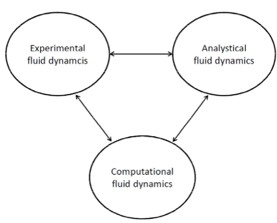
have the access to those high-performance computing facilities. Nowadays it has been a popular approach throughout the engineering applications, especially for aerospace and automotive engineering. Computational fluid dynamics has become a new third approach to offer a cost-effective alternative solution for the research in fluid dynamics (Anderson 1995). It complimented the other two approaches of experimental fluid dynamics and theoretical fluid dynamics to form a harmonic balance of tripod, each approach is equally important and irreplaceable to others, as shown in the Fig. 1.1.

which are based on the hypothesis of continuum, to the numerical simulation of microfluidic devices. In contrast, for the nanofluidics where the hypothesis of continuum is no longer valid, the molecular dynamics and quantum mechanics are required for numerical simulations.

Fig. 1.2 Effect of fluid volume on the density measured by an instrument (Batchelor 2000)

models while it is partially modelled in large eddy simulation depending on the grid sizes used in the simulation. If the grid size is refined smaller enough, the solution of large eddy simulation becomes similar to the solution of direct numerical simulation.

Fig. 1.3 the classification of turbulence modellings on the computation cost and resolved physics (Sagaut, Deck et al. 2006)

problem at hand, one often uses microtubes or microchannels as the first step for investigating the turbulent flows in microscale. In microchannel experiments, one fundamental question has attracted intensive researches in recent years: Whether the turbulent flow in the microchannel has the same characteristics as it has in the conventional channel. With the newly developed microscopic Particle Image Velocimetry (micro-PIV) technique the statistical and structural similarities of turbulence between microscale and macroscale channels are showed by Natrajan et al. and Li and Olsen. (Li and Olsen 2006, Natrajan, Yamaguchi et al. 2007). One of main reasons of early transition is attributed to the relatively high surface roughness in the microchannel (Natrajan and Christensen 2010). As the result, those turbulent models developed for the macroscale flow could be directly1 applied to the turbulent simulation in the microscale flow. However, to the best of this author’s knowledge, it is very rare2 to find the CFD researches of turbulent flow modelling in microchannel, even if not to mention the micromixer. The current majority of CFD researches are focusing on the regime of laminar

1 _{They might need some calibration}

1.4 Experiment of Laser-Induced Microscale

Cavitation Bubbles

developed flow measurement technique (Iben, Morozov et al. 2011). However, there are still many unknown effects of such micro-scale cavitation bubble, some of which are fundamental in the microfluidics. Without a full understanding of these microscale cavitation bubbles and their effects, developing next generation of such high performance mixers is impossible. To facilitate the design of continuous-flow micromixer, new approaches for investigating the dynamics of these micro bubbles have been proposed by this PhD programme.

1.5

Outline of Present Work

Chapter 2

Searching For Numerical Approach

Suitable for Microchannel Flows

2.1 Introduction

devices and are essential for further advancing microfluidic devices. Currently, the turbulent and transitional flows in the microchannel are a hot area of research owing to the discrepancies of experimental data between the conventional macroscale and microscale channels, which might be contributed to the unknown microscale effects involved. For example, some researchers have reported the deviations of friction factor observed in the microchannel indicating an earlier turbulence transition than it should be. Peng et al. (Peng, Peterson et al. 1994) observed an earlier turbulence transition occurring approximately at Reynolds numbers in the range of 200-700 and a fully turbulent flow at Reynolds numbers of 400-1500 in a rectangular microchannel3. Mala and Li (Mala and Li 1999) reported an earlier turbulent transition of water flowing through microtubes made of fused silica and stainless steel with size ranging from 50 to 245 um. The transitional and fully turbulent Reynolds numbers are, subject to materials used, ranging from 300-900 and fully developed turbulence of 1000-1500, respectively. In these reports, they concluded that the higher experimental

analytical estimation obtained from dimensional analysis and concluded no differences between conventional and microscale channels. Steinke and Kandikar (Steinke and Kandlikar 2006) reviewed over 150 papers from available literature that directly deal with the pressure drop measurement in microchannel. Based on approximately 40 papers that reported the detailed experimental data, they established a database with the total number of datum points over 5000 and concluded that the significant deviation from conventional theory are those papers not accounting for the entrance and exit losses or the frictional losses resulting from developing flow in the microchannel. With the correction of these component losses their experimental data show good agreements with the theory for the laminar flow. In addition to the above-mentioned reasons, the measurement accuracy that can contribute a large uncertainty in the experimental data (Judy, Maynes et al. 2002, Guo and Li 2003) is identified as another crucial factor causing the discrepancy.

micromixer.

transition in the rough silicon rectangular microchannel was also observed by Hao et al. (Hao, Yao et al. 2006). Through micro-PIV the structural similarities between macroscale and microscale wall turbulences were observed in both rectangular (Li and Olsen 2006b) and round (Natrajan, Yamaguchi et al. 2007) microchannels. The large turbulent eddies were observed directly in the instantaneous velocity fields showing the consistency with the large-scale turbulent structure often observed in the macroscale. In addition, the single-point velocity statistics including the mean velocity profile, the root-mean-square streamwise and wall-normal velocities, and the Reynolds stress profile can be computed from the instantaneous, statistically independent velocity fields acquired by micro-PIV, which also shows quite good statistical similarities with the results from direct numerical simulation. In conclusion, all the above results show that micro-PIV is a truly suitable tool for the investigation of microscale flow.

field in the near-wall region well, which greatly extends the attractiveness of micro-MTV and opens a new way to study the mean dynamics of transitional channel flow (Elsnab, Klewicki et al. 2011).

required turbulent flow at extremely high velocity while avoiding the leakage of microfluidics caused by the high pressure. The recent renaissance in the continuous flow micromixer has thus shown a desire for searching and developing a valid CFD approach for simulating turbulent flow including its transition in the microscale flow.

implementing LCTM with the experimental correlation into the general-purpose CFD code.

2010). All these successes demonstrate the great potential of this transition turbulence model.

2.2

Simulation Model

There are two models with different geometrics employed in our simulations. Case 1 is a rectangular micro-channel and case 2 is a circular micro-tube. The model geometries are such selected because they can be compared with available micro-PIV data in the literature (Li, Ewoldt et al. 2005, Li and Olsen 2006b, Natrajan, Yamaguchi et al. 2007). For case 1, it is a three-dimensional rectangular micro-channel with a width 320 µm and a height 330 µm. Its aspect ratio is 0.97 and hydraulic diameter is 325 µm. The length of micro-channel is 50,000 µm. The measured surface roughness of the microchannel from the experiment is approximately 24 nm in arithmetic average, which corresponds to 0.000074 of the relative roughness (Li and Olsen 2006b). This relative roughness has little effect on the flow investigated where the Reynolds number is below ₁₀4 _{such that the flow}

2.2.1 Governing Equations of LCTM

The numerical model employed here was devised by Menter et al. (Menter, Langtry et al. 2006a). The governing equation of LCTM is comprised of three sets of equations (Abraham, Sparrow et al. 2008). The first set represents the continuity equation and the Reynolds-averaged Navier-Stokes (RANS) equation.

(2.1)

(2.2)

where

Where ρ is the density and p is the pressure. u ,1 u ,2 u denote the 3 x1,x2,

3

x (i.e. x,y,z) components of mean flow velocity, respectively. μ and μ_turb

denote the viscosity and turbulent viscosity, respectively. The second pair represents the Shear Stress Transport (SST) turbulence model for kinetic energy and dissipation rate, which was also formulated by Menter (Menter 1994). The SST model yields the prediction of turbulent viscosity _{tu r b} for

eq. (2.2). 0 i i u x  _  1,2,3 j





 





j j

i turb

i i i i

u p u

u

x x x x

_  _     _    _

   

(2.4) Where P is the production rate of turbulent kinetic energy k and _k ωdenotes

the specific rate of turbulence destruction.  terms denote the prandtl numbers for the transport of k and ω. S denotes the absolute rate of shear strain rate. F₁ and F₂ denotes the blending function of SST model. α, β₁ and β₂ denote the SST model constants. Solving eq. (2.3) and (2.4), one can obtain the turbulence viscosity μ_turb in terms of k and ω.

2

max( , )

turb _SF

 



 (2.5)

To couple the turbulence model with the transition model, the SST model has been modified with the intermittency γ in production term P , which will _k

dampen the production term in the regions of laminar flow and turbulence intermittency. The last set of equations is the transport equations for the transition, i.e. the intermittency transport equation and transition momentum-thickness transport equation.

(2.6)

  2 2

2 1

2

1 2(1 )

i turb

i i i i i

u _{S F} k

x x  x  x x

  _{   }   _                _  _{ }    _{ } _  

,1 ,1 ,2 ,2

i turb

i i i

u

P E P E

t x     x _ x

(2.7)

where Re is transition momentum thickness Reynolds number. _θt P_,1 and

,2

P_ are the source terms of intermittency equation. E_,1and E_,2 are the

destruction term of intermittency transport equation. P_t is the source term

of transition momentum-thickness transport equation. The intermittency equation in eq. (2.6) is used for triggering the turbulence transition and turning on the production term in eq. (2.3) and the momentum-thickness transport equation in eq. (2.7) is used for connecting the transition onset criteria of the intermittency equation with the empirical correlation that is based on the relation between transition momentum thickness and strain-rate Reynolds number.

This Reynolds-averaged turbulence model can be used for predicting the mean fields of transitional turbulence flow as well as the laminar flow and fully turbulent flow to form a complete description of the Navier-Stokes equations. The model devised by Menter et al. was specifically for the external flow, which was based on the experimental correlation to calibrate the empirical constants for the applicability of this transition model. For

 

R e t i R e t R e t

t t tu r b

i i i

u

P

t x x x

  

 

  _{  } 

 _  _{ }  _ 

 

application to internal flow, the calibration of the empirical constants has to be done. Here, we have adapted the empirical constants from Abraham et al. (Abraham, Sparrow et al. 2008) , which are determined by systematic evaluation. The modifications of the model are an increase of constant C_γ,2,

appearing as a multiplier of E_γ2 in the intermittency equations, from 50 to 70

and a reduction of constant C_{θ, t}, appearing in the production term of the

transport equation, from 0.03 to 0.015. Although the empirical correlation and the transition model are originally devised in the conventional macroscale system, there are some statistical and structural similarities between microscale and macroscale in wall turbulence (Li and Olsen 2006a, Natrajan, Yamaguchi et al. 2007, Elsnab, Maynes et al. 2010). As the result, the empirical correlation method developed under the conventional system should offer the same capabilities for exploring the microscale system. For further details on the transitional model readers are referred to (Langtry, Menter et al. 2006, Menter, Langtry et al. 2006a, Menter, Langtry et al. 2006b).

13.0 and 14.0 softwares. CFX uses a coupled solver to solve the hydrodynamic equations simultaneously as a single system. A fully implicitly, false transient, and time-stepping algorithm is used for approaching the steady state solution which reduces the number of iterations for achieving convergence. For reducing the source of solution errors a high resolution advection scheme has been adapted for all equations including hydrodynamic equations, turbulent equations and transitional equations. It gives a dynamic adjustment and better trade-off between the order of accuracy and the robustness. The method developed by Rhie and Chow (Rhie and Chow 1983) and modified by Majumdar (Majumdar 1988) has been adapted by CFX for avoiding the velocity-pressure decoupling, which imposes the velocity-pressure coupling equation onto the non-staggered grid layout and removes the dependence of the steady-state solution on time step. A high resolution scheme is also adapted for the Rhie Chow pressure dissipation algorithm.

the fully developed region is used for comparing with those obtained from the literature. The criterion of convergence has been set for residual values of

6

10

except for the intermittency residual value of ₁₀5_.

2.2.3

Mesh Independence Study

Fig. 2.1 The mesh independency for rectangular channel case.

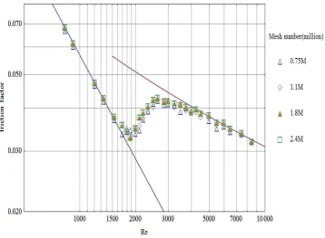
Reynolds numbers investigated such that all the near-wall elements are resolved properly. The mesh independency study is shown in Fig. 2.1 for the rectangular micro-channel case. The mesh independency has been achieved when the mesh number increase to 1.8 millions.

2.3

Result and Discussion for the Simulation

of Rectangular Microchannel

The results obtained from the simulation are compared with those from the literature. In particular, the friction factor is used for the validation of our simulation. Through numerical simulation, one can obtain enormous and complete fluid dynamics data to be used for the elucidation of the flow behaviours both quantitatively and qualitatively. Furthermore, we use the velocity profile obtained from the simulation for the analysis against the results obtained from micro PIV in the literature.

2.3.1

Friction Factor of Fully Developed Flows

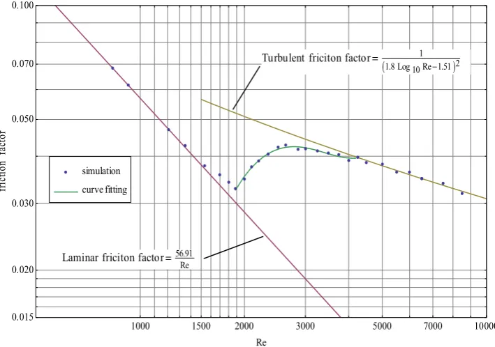
defined as the Reynolds number based on the inlet velocity and the hydraulic diameter. The friction factor calculated from fully developed flow region covering laminar, transitional turbulent and fully turbulent regimes as plotted in Fig. 2.2. The dots represent the friction factor obtained from our simulation. The result is compared with the data from White (White 2008) where laminar friction factor based on the analytical solution is used for the comparison in laminar flow regime; and, for fully turbulent regime, turbulent friction factor based on an empirical equation developed by Haaland (Haaland 1983) is used, which is an explicit and simplified form of Colebrook-White formula. Figure 2.2 indicates that the model has accurately simulated the friction factor in both the laminar and fully turbulent regimes, for which the model is validated. In the transitional turbulent regime, the simulation data can be fitted as a polynomial equation as shown in eq. (2.8).

_{f = -0.186+2.51 10 Re-10 Re +1.72 10 Re -1.08 10 Re}-4 -7 2 -11 3 -15 4

tr   

prediction of turbulence transition. The solid line in transitional turbulent regime represents the fitting equation which predicts the friction factor of turbulence transition in the rectangular micro-channel.

Fig. 2.2 Rectangular case: the computed friction factor compared with the moody chart

2.3.2 Velocity

Profile

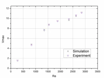
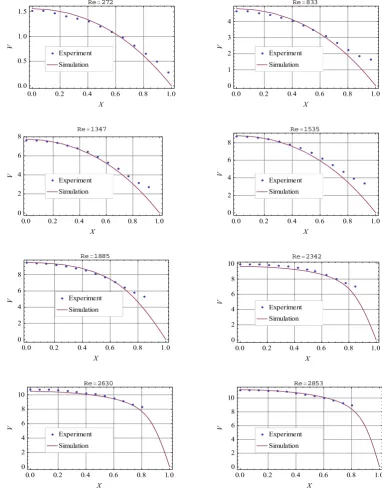
Since there is no well-defined and accurate theory for predicting the friction factor in the transitional turbulent regime that could be used for comparison, instead we have employed the maximum velocity and corresponding velocity profile obtained from micro-PIV studies for comparison. Figure 2.3 shows the comparison of maximum velocities. The experimental data are obtained

1000 1500 2000 3000 5000 7000 10000 0.100

0.050

0.020 0.030

0.015 0.070

Re

fr

ict

io

n

fa

ct

or

curve fitting simulation

Laminar friciton factor=56.91

Re

from Li et al. ( Li, Ewoldt et al. 2005) and Li and Olsen (Li and Olsen 2006b).

Fig. 2.3 The maximum velocity of fully developed flow

shown below.

Fig. 2.4 various velocity profiles of fully developed flow against the normalized width of channel

The further comparison of velocity profiles between the experiment and the simulation is shown in Fig. 2.4. The abscissa represents the normalized width

0.0 0.2 0.4 0.6 0.8 1.0

0.0 0.5 1.0 1.5 X V

Re272

Simulation Experiment

0.0 0.2 0.4 0.6 0.8 1.0

0 1 2 3 4 X V

Re833

Simulation Experiment

0.0 0.2 0.4 0.6 0.8 1.0 0 2 4 6 8 X V

Re1347

Simulation Experiment

0.0 0.2 0.4 0.6 0.8 1.0

0 2 4 6 8 X V

Re1535

Simulation Experiment

0.0 0.2 0.4 0.6 0.8 1.0

0 2 4 6 8 X V

Re1885

Simulation Experiment

0.0 0.2 0.4 0.6 0.8 1.0

0 2 4 6 8 10 X V

Re2342

Simulation Experiment

0.0 0.2 0.4 0.6 0.8 1.0

0 2 4 6 8 10 X V

Re2630

Simulation Experiment

0.0 0.2 0.4 0.6 0.8 1.0

0 2 4 6 8 10 X V

Re2853

of channel from the centre of channel where the abscissa is designated as 0 to the wall of channel where the abscissa is designated as 1; whereas, the ordinate represents the velocity of flow in the fully developed region. The maximum velocity of flow occurs at the centre of channel; the minimum velocity occurs at the wall of channel.

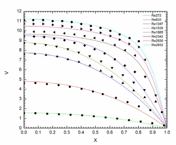
Fig. 2.5 Velocity profiles ranging from Reynolds number 272 to 2853

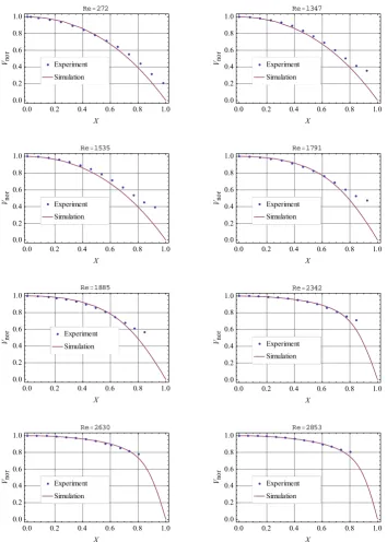
Fig. 2.6 Various normalized velocity profile against the normalized width of channel

While the Reynolds number increases, the profiles start deviating from the laminar parabolic solution towards the turbulent logarithmic solution, i.e. the third group. This deviation happens from Reynolds number 1885 which

0.0 0.2 0.4 0.6 0.8 1.0 0.0 0.2 0.4 0.6 0.8 1.0 X Vno r

Re272

Simulation Experiment

0.0 0.2 0.4 0.6 0.8 1.0 0.0 0.2 0.4 0.6 0.8 1.0 X Vno r

Re1347

Simulation Experiment

0.0 0.2 0.4 0.6 0.8 1.0 0.0 0.2 0.4 0.6 0.8 1.0 X Vno r

Re1535

Simulation Experiment

0.0 0.2 0.4 0.6 0.8 1.0 0.0 0.2 0.4 0.6 0.8 1.0 X Vno r

Re1791

Simulation Experiment

0.0 0.2 0.4 0.6 0.8 1.0 0.0 0.2 0.4 0.6 0.8 1.0 X Vno r

Re1885

Simulation Experiment

0.0 0.2 0.4 0.6 0.8 1.0 0.0 0.2 0.4 0.6 0.8 1.0 X Vno r

Re2342

Simulation Experiment

0.0 0.2 0.4 0.6 0.8 1.0 0.0 0.2 0.4 0.6 0.8 1.0 X Vno r

Re2630

Simulation Experiment

0.0 0.2 0.4 0.6 0.8 1.0 0.0 0.2 0.4 0.6 0.8 1.0 X Vno r

Re2853

indicates the beginning of turbulence transition. This value of Reynolds number is also indicated from the graph of friction factor, referring to Fig.2.3. Though the shape deviation can be identified for the Reynolds number between 1700 and 1885, they still maintain a quasi-parabolic shape, as also indicated in the graph of friction factor. Immediately after Reynolds number reaches 1885, the burst of the turbulence transition starts corresponding to a sudden jump of the friction factor.

Fig. 2.7 Normalized velocity profiles ranging from Reynolds number 272 to 2853

with the variation of friction factor. That is if the friction factor varies fast, the shape of velocity profile will also changes fast such as for the Reynolds number between 1885 and 2630. On contrast, the shape variation slows down after the Reynolds number of 2630 where the corresponding friction factor also changes slowly. In the fully turbulent regime where the Reynolds number exceeds 4250, as indicated by Fig. 2.2, the variation of shape against Reynolds number becomes much slower and even negligible.

Fig. 2.8 Normalized velocity profiles ranging from Reynolds number 1347 to 8500

These comparisons indicate that our approach established based on the local

æ æ æ æ æ æ æ æ æ æ æ æ æ æ æ æ æ æ æ æ æ æ æ æ æ æ æ æ æ æ æ æ æ æ æ æ æ æ æ æ æ æ æ æ æ æ æ æ æ æ à à à à à à à à à à à à à à à à à à à à à à à à à à à à à à à à à à à à à à à à à à à à à à à à à à ì ì ì ì ì ì ì ì ì ì ì ì ì ì ì ì ì ì ì ì ì ì ì ì ì ì ì ì ì ì ì ì ì ì ì ì ì ì ì ì ì ì ì ì ì ì ì ì ì ì ò ò ò ò ò ò ò ò ò ò ò ò ò ò ò ò ò ò ò ò ò ò ò ò ò ò ò ò ò ò ò ò ò ò ò ò ò ò ò ò ò ò ò ò ò ò ò ò ò ò ô ô ô ô ô ô ô ô ô ô ô ô ô ô ô ô ô ô ô ô ô ô ô ô ô ô ô ô ô ô ô ô ô ô ô ô ô ô ô ô ô ô ô ô ô ô ô ô ô ô ç ç ç ç ç ç ç ç ç ç ç ç ç ç ç ç ç ç ç ç ç ç ç ç ç ç ç ç ç ç ç ç ç ç ç ç ç ç ç ç ç ç ç ç ç ç ç ç ç ç á á á á á á á á á á á á á á á á á á á á á á á á á á á á á á á á á á á á á á á á á á á á á á á á á á í í í í í í í í í í í í í í í í í í í í í í í í í í í í í í í í í í í í í í í í í í í í í í í í í í ó ó ó ó ó ó ó ó ó ó ó ó ó ó ó ó ó ó ó ó ó ó ó ó ó ó ó ó ó ó ó ó ó ó ó ó ó ó ó ó ó ó ó ó ó ó ó ó ó ó õ õ õ õ õ õ õ õ õ õ õ õ õ õ õ õ õ õ õ õ õ õ õ õ õ õ õ õ õ õ õ õ õ õ õ õ õ õ õ õ õ õ õ õ õ õ õ õ õ õ æ æ æ æ æ æ æ æ æ æ æ æ æ æ æ æ æ æ æ æ æ æ æ æ æ æ æ æ æ æ æ æ æ æ æ æ æ æ æ æ æ æ æ æ æ æ æ æ æ æ à à à à à à à à à à à à à à à à à à à à à à à à à à à à à à à à à à à à à à à à à à à à à à à à à à ì ì ì ì ì ì ì ì ì ì ì ì ì ì ì ì ì ì ì ì ì ì ì ì ì ì ì ì ì ì ì ì ì ì ì ì ì ì ì ì ì ì ì ì ì ì ì ì ì ì ò ò ò ò ò ò ò ò ò ò ò ò ò ò ò ò ò ò ò ò ò ò ò ò ò ò ò ò ò ò ò ò ò ò ò ò ò ò ò ò ò ò ò ò ò ò ò ò ò ò ô ô ô ô ô ô ô ô ô ô ô ô ô ô ô ô ô ô ô ô ô ô ô ô ô ô ô ô ô ô ô ô ô ô ô ô ô ô ô ô ô ô ô ô ô ô ô ô ô ô

0.0 0.2 0.4 0.6 0.8 1.0

correlation-based transition model is suitable for the simulation of transitional turbulence flow in the micro-channel, in particular with the rectangular cross-section. This approach has thus filled up the gap of simulation between the laminar and fully turbulent flows.

2.3.3 Flow

Development

along Streamwise Direction

Various information of flow field can be obtained from the numerical simulation, which facilitates a better understanding of fluid dynamics in microchannel. Figure 2.9 shows the flow development of the ratio of maximum velocity to mean velocity V_max V_ave in the streamwise direction

throughout the entire flow regimes. The streamwise axis is normalized by the hydraulic diameter d_h. The three different behaviours of flow are presented

the Reynolds numbers of flow increase. Immediately after the breakdown of initial laminar development, the fully turbulent flows, i.e. Re=5000 and 6000, attain the fully developed flow very quickly.

Fig. 2.9 The streamwise flow development of the ratio of maximum velocity to mean velocity

Another flow characteristic predicted by LCTM transitional model is the development of turbulent eddy viscosity _turb _m , i.e. normalized by

molecular viscosity, against the streamwise direction as shown in Fig. 2.10. Although a turbulent intensity of 5 %, i.e. _turb _m10 is set as the default

decays immediately in very short distance and is suppressed successfully to 0 in the laminar flow case. Whereas, In the cases of transitional turbulent and fully turbulent flows, the turbulent eddy viscosity grows steadily with the increase of Reynolds number.

Fig. 2.10 The streamwise flow development of eddy viscosity

2.4

Result and Discussion for the Simulation

of Micro-tube

transitional, and fully turbulent flow regimes. As shown in Fig. 2.11, the friction factors calculated from simulation data are also compared with the Moody chart as for the rectangular case. The theoretical friction factor of circular tube shown as the solid line in laminar regime and the turbulent friction factor obtained from the empirical Colebrook-White formula shown as the solid line in fully turbulent regime are used for comparison. Whereas, the dots between the laminar and fully turbulent regimes are the calculated friction factor obtained from the simulation.

Fig. 2.11 Circular case: the computed friction factor compared with the Moody chart

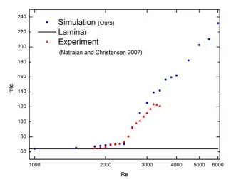
between our simulation data and the empirical formula as well as the laminar theoretical prediction. The pipe flow characteristics simulated by this LCTM transition model is accurately predicted, though with a slight deviation in quantity. In the paper of Natrajan and Christensen (Natrajan and Christensen 2007), by varying flow rate, the pressure drops across the micro-tube against various Reynolds numbers were measured. These measured data of pressure drop and friction factor were compared with conventional laminar theory as well as the experimental results obtained from Sharp and Adrian (Sharp and Adrian 2004).

Fig. 2.13 Circular case: the comparison between the computed friction factors (ours) and experimental data from the published literature (Natrajan and Christensen 2007)

2.5

Summary

Chapter 3

Numerical Simulation of Micromixer

3.1

Introduction

diffusion, chaotic advection, and turbulent diffusion as illustrated in Fig. 3.1. The continuous-flow micromixer utilising the turbulent mixing is superior over those discussed previously in the introductory chapter.

erosion on micromixer itself. All of these issues cause the difficulties in investigating turbulent micromixer experimentally. Moreover, lack of experimental data in validating and calibrating a suitable numerical approach makes the CFD studies on turbulent micromixer more difficult.

The mixing mechanism of micromixer in the laminar flow condition mainly relies on the flow convection and molecular diffusion. For more details on various types of laminar and chaotic micromixers the readers are referred to the book (Nguyen 2012). As the in-flow velocity of fluids is low4, i.e. the Reynolds number is smaller than 10, the mixing is mainly dominated by molecular diffusion. As the Reynolds number becomes higher than this value, the mixing is mainly dominated by convection. A review and classification on the laminar and chaotic flow mixing with the characteristics of their flow pattern is given by Kockmann (Kockmann 2008b). As the Reynolds numbers are increased from 0.01 to 1000, the flow patterns in the mixing channel also varies in sequence, such as from laminar straight streamline, symmetric

vortex flow, engulfment flow5, periodic pulsating flow, and chaotic pulsating flow. Within this range of Reynolds number, the mixing mechanism is being transformed from laminar diffusion throughout to chaotic convection. These changes on the flow pattern are mainly caused by the induced hydrodynamic instability, i.e. Kevin-Helmholtz instability, which is resulted from the high shear flow between the contact areas of two fluids. This instability leads to the unstable flow condition and periodic fluctuating behaviours of flow. Eventually, the chaotic mixing of flow structure is obtained as the Reynolds number is approximately greater than 500. These classifications are also illustrated by Kockmann (Kockmann 2008a) as illustrated in Fig. 3.2.

Fig 3.2 The classification of flow regimes on 1:1 mixing by Kockmann (Kockmann 2008a)

5 _{The engulfment flow refers to the breakdown of symmetric vortex flow becoming as}

T-junction micromixer is employed as the geometric model for simulating and characterizing the flow. As for the discrimination on the mixing quality of a micromixer, the segregation of intensity is employed for quantitatively analysing the simulated micromixer. This numerical approach provides us a CFD tool for guiding and optimising the design of turbulent micromixer.

3.2

Governing Equations of Numerical

Simulation for the Micromixer

In order to evaluate the degree of mixing, a passive scalar tracer that has no effect on the material properties such as dye is often used in the experiment of mixing. By utilising the conservation law of species one can derive a convection-diffusion equation to simulate the transport of this scalar property in the micromixer. This scalar transport equation that characterises the convection6 and molecular diffusion is written as

2

2 , 1 ~ 3

i m

i i

c c c

u D i

t x x

 _  _  _

_{ }  _

  (3.1)

where c denotes the concentration field of scalar material and D_m denotes

the kinematic diffusivity7, i.e. the coefficient of molecular diffusion determined by the material properties. The term in the right hand side represents the mixing caused by molecular diffusion. The first and second terms in the left hand side represent the time dependence and convection of scalar field, respectively.

By utilising the concept of Reynolds decomposition, the mixture fraction and velocity can be divided into the fields of mean flow and fluctuating flow.

 

   

 

 

 

, , ,

, , ,

i i i

i i i

c x t c x t c x t u x t u x t u x t

   

 



 

 (3.2)

Inserting eq. (3.2) into eq. (3.1), one can obtain

i 2₂

i m

i i i

c c u c c

u D

t x x x

  

 _  _ _ 

 

 _   _  (3.3)

modelled. Using the assumption of Reynolds analogy used for Reynolds stress, the scalar flux is assumed to be proportional to the gradient of the mean scalar field c, i.e. the gradient-diffusion hypothesis, i.e. the fick’s law of molecular diffusion.

_{i turb}

i c

u c D

x

    

 (3.4)

where D_turb is turbulent diffusivity8, the effective mass diffusion coefficient

due to turbulence. By inserting eq. (3.4) into eq. (3.3) the convection Diffusion equation with turbulent diffusion9 can be obtained





2

,

1 ~ 3

i m turb

i i

c

c

c

u

D

D

i

t

x

x



_



_

_



_







For details on the derivation and discussion on the convection-diffusion equation, readers are referred to books, e.g. (Bird, Stewart et al. 2007) and (Cussler 2009).

8 _{Note that the turbulent diffusivity is assumed to be isotropic for simplifying the problem.} 9 _{Note that for the conciseness the overbars for cand}

i

Combining this equation together with LCTM transition model allows us to simulate the scalar transport in the micromixer throughout the entire flow regime including laminar, turbulence transitional, and fully turbulent flows. As discussed previously in the chapter two, the governing equations of LCTM are consisted of three sets of equations. The first set is the continuity equation and the RANS equation. The second set, i.e. the SST turbulence model which predicts the turbulent viscosity, is coupled with the third set of equations, the essential part of LCTM transition model. The LCTM model corrects the prediction of turbulent viscosity and mean flow velocity based on an empirical formula for different flow regimes, especially for the regime of laminar-turbulent transition. In this study, the convection-diffusion equation is connected with the LCTM transition model by the velocity field of flow and the coefficient of turbulent diffusivity D_turb. In eq. (3.5), the coefficient

of turbulent diffusivity is taken as

t turb

t

D

Sc 

 (3.6)

where _t is turbulent viscosity and Sc_t is turbulence Schmidt number,

momentum diffusivity to the turbulent mass diffusivity. In order to simplify the problem, Sc_t is fixed as 0.9 in our study and this empirical constant

number10 will be used in all our simulations using LCTM transition model since our aim, here, is to demonstrate and exemplify a viable numerical approach for tackling and evaluating rapid mixing in micromixer, especially for those in the transition-turbulent and fully turbulent regime. Furthermore, as shown in Fig. 2.10, the turbulent viscosity calculated by LCTM transition model is damped to zero in the laminar flow regime as the flow is fully developed. Therefore, the turbulent term in eq. (3.5) thus disappears and resulting in a convection-diffusion equation for laminar flow.

3.3

Evaluation of Micromixer by Mixing

Quality

In order to evaluate the mixing quality of a micromixer, a concept for measuring the intensity of segregation is defined by Danckwerts (Danckwerts 1958). The segregation in a mixture means that some parts of mixture contain

10 _{The value 0.9 is a non-universal empirical constant number generally adopted in CFD}

a higher concentration of material than the average concentration in the mixture. The Danckwerts’ intensity of segregation I_s that describes a

relative variance of the concentration in a mixture is as follows.

2

2 max

s

I 



 , 2





A

c c dA

 

_

where



max

 is a reference value for the normalization,

which can be defined as the maximum possbile variance as shown by eq. (3.8)

or as the variance at the initial time or at the entrance of mixing channel (Bothe, Stemich et al. 2008).

2





   (3.8)

_

_

2

1

s I

a a







,





2

2 1

A

a a dA A

 

_

Herein, a measure for the intensity of segregation IM is given as

max

1 1

M S

I I 



    (3.10)

where IM varies from the value of one to zero, corresponding to

homogeously mixing and completetly segregated states, respectively. For more detail discussion on the evaluation of mixing quality, readers are referred to the book (Bockhorn, Mewes et al. 2010).

3.4 Mixing Simulation Using LCTM Transition

Model for T-junction Micromixer

in-flow channels in the junction where the in-flow and out-flow channels are joined together. After a bend of 90 degree on the direction of both fluids, the joining fluids are mixed as it flows through the out-flow channel, i.e. the mixing channel of micromixer.

Fig. 3.3 Illustration of T-Mixer

The geometric model we used here is a typical T-junction micromixer with a rectangular cross-section of 100 by 100 µm11 across the entire micromixer where the hydraulic diameter12

h

D is 100 µm. The T-mixer is 5 D_h long in

11 _{i.e. the symmetrical 1:1 mixing.} 12 _{The hydraulic diameter}

h

D is defined as 4A

the inlet channels and 100 D_h long in the outlet channel. The numerical

implementation is realized by the CFD software, ANSYS CFX, as discussed in the chapter 2. The mesh requirement is taken to be the same criteria as the micro-channel simulation in the chapter 2. Approximately 1,060,711 nodes are deployed with 1,008,000 elements for the simulation of micromixer. The special criterion y_1 _{is fulfilled to resolve the near-wall behaviour of flow}

for all the simulation along the stream-wise location. Firstly, we implement the laminar flow simulation to examine the mixing quality of this T-junction micromixer.

In Fig. 3.4, the mixing efficiency of simulated micromixer at distance of 2000 um after the flow enters mixing channel is shown against Reynolds number13. It shows that the mixing quality are high as the Reynolds numbers are either extremely low or higher enough. This is because as the flow velocity is extremely slow, the fluids has a very long residence time to diffuse in the mixing channel. However, To complete the mixing, attaining a high mixing

efficiency, would require a huge amount of time. For example, in this case, it would take approximately 1.57 s for the flow of Reynolds number 0.01 to arrive at the location of 2000 um in the mixing channel whereas it only takes 15 us for the flow of Reynolds number 750.

Fig. 3.4 Mixing efficiency against Reynolds number (laminar simulation)

relatively low because there is no enough time for diffusion of the (virtually) straight laminar structure of flow in the mixing channel. For details of discussion on these flow characteristics, please refer to (Kockmann 2008b).

Fig. 3.5 Mixing efficiency against the length of mixing channel (laminar simulation)

fluctuating flow behaviours in the mixing channel. Therefore, the results for Reynolds number 500 and 750 shown in Fig. 3.5 have been time-averaged. In this chapter, all the results obtained by transient simulation has been averaged by numerous instantaneous results of simulations in order to present the expecting value of mixing efficiency obtained from unsteady flow structures.

Fig. 3.6 Overview on the fluids mixing along the mixing channel from Reynolds number 0.01 to 5 (laminar flow model)

In Fig. 3.6 the fluids mixing from Reynolds number 0.01 to 5 with the view of cross-sections parallel to mixing channel is shown. The red and blue colours represent 1 (with the dye) and 0 (without the dye), respectively. As the colour is turned into green (i.e. 50:50), representing an evenly mixture14.

Re=0.01 Re=0.5

Figure 3.6 indicates that the mixing quality is very high for the case of Reynolds number 0.01 and is low for the rest of cases because the mixing here only relies on molecular diffusion as discussed before.

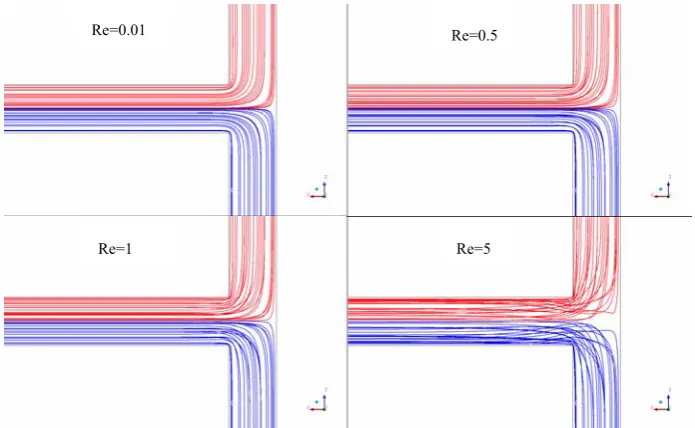
In Fig. 3.7 the streamlines of flow in the micromixer from Reynolds number 0.01 to 5 are shown. Under this flow regime, all the streamlines simply stays as straight laminar flow in the mixing channel without any vortex structure. The fluids flow through the mixing channel symmetrically even without any entanglements of streamlines. Therefore to design this type of micromixer, designers should focus on reducing the striation thickness of fluids, i.e. increasing the contact area between fluids by various measures.

Fig. 3.7 Overview on the streamlines of flow along the mixing channel from Reynolds number 0.01 to 5 (laminar flow model)

Re=0.01 _Re=0.5

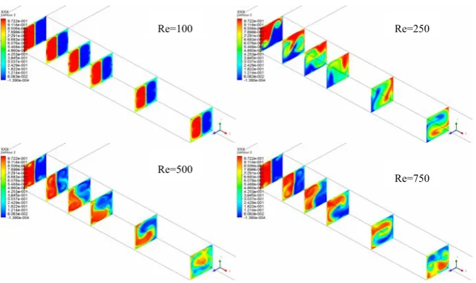
In Figs. 3.8 and 3.9, the fluids mixing from Reynolds number 100 to 750 with the views of cross-sections that are parallel and perpendicular to mixing channel is shown, respectively. Note that for the cases of Reynolds number 500 and 750, the transient results are displayed.

Fig. 3.8 Overview on the fluids mixing with the view of cross-sections parallel to mixing channel from Reynolds number 100 to 750 (laminar flow model)

Fig. 3.9 Overview on the fluids mixing with the view of cross-sections perpendicular to

Re=100 Re=250

Re=500 Re=750

Re=100 Re=250

Re=500

As the Reynolds number is increased, the vortices generated by the convection of flow further enhance the mixing quality of fluids. One thing worth noting is that the mixing quality for Reynolds number 250 goes up quickly within a very short distance as shown in Fig. 3.5. This is because the roll-up vortices induced by the convection of flow happens at the interface of fluids as shown in Fig. 3.9, greatly enhancing the mixing. This indicates that an ideal flow structure could be generated through the convection mechanism even in the laminar flow to plays a significant role for promoting mixing.

Fig. 3.10 Overview on the streamlines of flow along the mixing channel from Reynolds number 100 to 750 (laminar flow model)

In Fig. 3.10, the streamlines of flow from Reynolds number 100 to 750 are shown. It illustrates that the vortices has been generated for the flow of

Re=100 Re=250

Reynolds number 100. however, the vortices remain aside its own fluid instead of interplaying with each other. For the rest cases, the interplay of vortices created by convection produces the intricate entanglement of streamlines.

In Fig 3.11, the streamlines of flow from Reynolds number 100 to 750 viewed from the entrance to exit of mixing channel clearly illustrates the evolution and complexity of streamlines entanglement.

Fig. 3.11 The streamlines of flow viewed from the entrance to exit of mixing channel (laminar flow model)

Recent progress on the continuous-flow micromixer as introduced in the first chapter has shown that there is no upper limit of Reynolds number for such a

Re=250

Re=500 Re=100

micromixer. As the critical Reynolds number for turbulence transition is exceeded, the onset of turbulent flow is triggered and turbulence structure is to be developed. The mixing mechanisms of micromixer in such flow conditions are dominated by molecular diffusion, flow convection and turbulent diffusion. For these mixing flows in micromixer, simulations by using Reynolds-averaged Navier-Stokes turbulence modelling was not possible until this approach presented in this thesis by using LCTM coupled with convection-diffusion equation. Now let us further discuss the contour of flow mixings obtained by this numerical approach firstly investigated by this PhD programme for turbulence micro-mixers.

mixing quality during a much shorter time.

Fig. 3.12 The mixing efficiency against Reynolds number (LCTM)

The mixing qualities against X obtained from these two models is also investigated as shown in Fig. 3.15. These two curves start to deviate from Reynolds number 100 reaching a maximum of 12.3% at Reynolds number 250.

Fig. 3.15 Comparison on mixing efficiencies calculated by both models against mixing channel

appropriated and quantitative comparison. And it is difficult to sat which model caused the discrepancy, though the LCTM approach is more rational. Therefore, future experimental validation is essential. Nevertheless, these simulated results are still valuable for qualitative discussion, providing guidelines for designing the micromixer for the rapid mixing applications.

Now let us further discuss the LCTM contour of flow mixing in comparison with those of laminar model (referring to Fig. 3.8). In Fig. 3.16, LCTM contours are shown along the mixing channel for Reynolds number 100 to 750. For Reynolds number 100 and 250, the contour patterns from both models are highly resemble.

Fig. 3.16 Overview on the fluids mixing along the mixing channel from Reynolds number 100 to 750 (LCTM)

Re=500

Re=100 Re=250