RESEARCH ARTICLE
Variation in hearing within a wild population of beluga whales
(
Delphinapterus leuca
s)
T. Aran Mooney1,*, Manuel Castellote2,3, Lori Quakenbush4, Roderick Hobbs3, Eric Gaglione5and Caroline Goertz6
ABSTRACT
Documenting hearing abilities is vital to understanding a species’ acoustic ecology and for predicting the impacts of increasing anthropogenic noise. Cetaceans use sound for essential biological functions such as foraging, navigation and communication; hearing is considered to be their primary sensory modality. Yet, we know little regarding the hearing of most, if not all, cetacean populations, which limits our understanding of their sensory ecology, population level variability and the potential impacts of increasing anthropogenic noise. We obtained audiograms (5.6–150 kHz) of 26 wild beluga whales to measure hearing thresholds during capture–release events in Bristol Bay, AK, USA, using auditory evoked potential methods. The goal was to establish the baseline population audiogram, incidences of hearing loss and general variability in wild beluga whales. In general, belugas showed sensitive hearing with low thresholds (<80 dB) from 16 to 100 kHz, and most individuals (76%) responded to at least 120 kHz. Despite belugas often showing sensitive hearing, thresholds were usually above or approached the low ambient noise levels measured in the area, suggesting that a quiet environment may be associated with hearing sensitivity and that hearing thresholds in the most sensitive animals may have been masked. Although this is just one wild population, the success of the method suggests that it should be applied to other populations and species to better assess potential differences. Bristol Bay beluga audiograms showed substantial (30–70 dB) variation among individuals; this variation increased at higher frequencies. Differences among individual belugas reflect that testing multiple individuals of a population is necessary to best describe maximum sensitivity and population variance. The results of this study quadruple the number of individual beluga whales for which audiograms have been conducted and provide the first auditory data for a population of healthy wild odontocetes.
KEY WORDS: Noise, Marine mammal, Cetacean, Odontocete, Arctic
INTRODUCTION
Underwater hearing and sound production are of primary importance for many marine taxa and these sensory modalities
are essential for communication, navigation, predator avoidance and foraging. Aquatic hearing is perhaps best understood for odontocetes (i.e. toothed whales) (Thomas et al., 2004; Au and Hastings, 2009). These animals produce complex acoustic signals, some individuals are known to have particularly sensitive aquatic hearing, and all have highly derived ears, which identify them as bioacoustic specialists (Au, 1993, 2000; Mooney et al., 2012).
Cetaceans are difficult to access for research; therefore, most studies of sound sensitivity include audiograms of just a few
individuals [e.g. bottlenose dolphins (Tursiops truncatus) (Johnson,
1967), white-beaked dolphins (Lagenorhynchus albirostris)
(Nachtigall et al., 2008), Blainville’s beaked whales (Mesoplodon
densirostris) (Pacini et al., 2011), Gervais’ beaked whales
(Mesoplodon europeaus) (Finneran et al., 2009) and
rough-toothed dolphins (Steno bredanensis) (Mann et al., 2010)].
Although data from an individual within a species are valuable and allow for initial comparisons of hearing abilities across species (Nachtigall et al., 2000; Mooney et al., 2012), they do not provide information on the variability within a species or population, making it difficult to place that audiogram in a biologically relevant context and potentially impeding the needs of population-relevant management (National Academy of Sciences, 2005).
The odontocetes for which we have the most audiograms are those in human-care facilities [e.g. bottlenose dolphins, killer whales, harbor porpoise (Johnson, 1966; Szymanski et al., 1999; Kastelein et al., 2002; Branstetter et al., 2017)]. Recent hearing studies have used physiological auditory evoked potentials (AEPs) to measure hearing thresholds, which allows hearing to be measured rapidly with untrained animals (reviewed in Nachtigall et al., 2007; Mooney et al., 2012), so that natural hearing abilities, hearing loss and individual variation within a species (Cook and Mann, 2004; Houser and Finneran, 2006b; Castellote et al., 2014) can be measured in more individuals and in wild settings. Although AEPs and portable measurement systems have opened the doors for substantially more auditory research, measuring audiograms in the field is still not an easy task, with challenges including animal access, acquiring healthy animals, safely maintaining animals, calibrations and sound presentation in uncontrolled environments, electrical noise, acoustic noise, weather, corrosion and effects of saltwater, repairs in the field, and difficulties associated with measuring neurological responses on the scales of microvolts, among others (Mooney et al., 2016). Thus, we are still data limited, with no population level audiogram assessments of healthy wild marine mammal populations.
Our current understanding of hearing variability at the population level largely comes from bottlenose dolphins in human care (Houser and Finneran, 2006b; Houser et al., 2008; but see Branstetter et al., 2017), where hearing can be associated with demographic and life history information of the individuals measured and it may be possible to relate some hearing loss to factors such as increasing age, effects of illness and medical treatment. Notably, Popov et al. (2007)
Received 17 October 2017; Accepted 12 March 2018
1Biology Department, Woods Hole Oceanographic Institution, Woods Hole, MA
02543, USA.2Joint Institute for the Study of the Atmosphere and Ocean (JISAO),
University of Washington, Seattle, WA 98105, USA.3Marine Mammal Laboratory,
Alaska Fisheries Science Center, National Marine Fisheries Service, Seattle, WA 98115, USA.4Alaska Department of Fish and Game, Fairbanks, AK 99701, USA. 5Georgia Aquarium, Atlanta, GA 30313, USA.6Alaska SeaLife Center, Seward,
AK 99664, USA.
*Author for correspondence (amooney@whoi.edu)
T.A.M., 0000-0002-5098-3354
Journal
of
Experimental
measured the hearing of 14 wild-caught bottlenose dolphins which
were maintained in a managed research facility for 3–5 months. The
animals had generally sensitive hearing, with a mean threshold
below 50 dB re. 1μPa at 45 and 54 kHz, and little to no detectable
age-related hearing loss (although they were thought to be relatively young, i.e. less than 15 years), with all but one hearing up to 152 kHz. Although preliminary, the data suggest that some odontocete populations may have sensitive hearing across a broad range of frequencies.
Thus, it seems vital to address and quantify natural hearing variability for healthy wild populations, a necessary component for estimating the population level consequences of noise (Hildebrand, 2009). Although audiograms of stranded animals can provide some information for natural populations, the reasons for stranding (e.g. old age, poor health) call into question the reliability of the data that may or may not represent the population (Nachtigall et al., 2005; Finneran et al., 2009; Mann et al., 2010). If stranded animals are likely to be older, the sample may represent a higher proportion of animals with presbycusis. Indeed, it has been reported that for some odontocete
populations, depending upon the species, 36–57% of stranded
animals tested have significant hearing deficits (Mann et al., 2010). Understanding natural hearing abilities at the population level is fundamental to addressing potential noise impacts such as masking, and potential noise-induced hearing loss at a time when anthropogenic noise is increasing in the marine environment. Larger sample sizes of individuals within a population provide improved data for estimates of the number of noise-related takes, i.e. the number of animals potentially affected by certain noise types. Such information can allow improved evaluations of noise-related impacts, which may include the probable frequencies of natural and potential noise-induced hearing loss and the probability of masking by certain noise types.
Like many areas in the world’s oceans, levels of man-made noise
are increasing in the Arctic and at high latitudes (Blackwell and Greene, 2002). Sources are varied and include seismic exploration for hydrocarbons, military activity including sonar and impulse noises of explosions, underwater construction such as pile driving and shipping through the Bering, Chukchi and Beaufort seas as a result of longer sea ice-free seasons and less ice overall, potentially making the great circle route and the northwest passage more economical (Beauregard-Tellier, 2008; Wang and Overland, 2009; Titley and St. John, 2010). Geophysical seismic activity has been described as one of the highest amplitude man-made underwater noise sources, with the potential to disturb or harm marine mammals including belugas (Heide-Jørgensen et al., 2013). Endangered Cook Inlet belugas, which have habitats close to Anchorage, AK, USA, can be exposed to noise from shipping, pile driving and other construction sounds, and explosive noise from nearby military bases (Blackwell and Greene,
2002; Norman, 2011). As these and other activities increase in high latitudes, anthropogenic noise will proliferate, permeating habitats for Arctic species and increasing potential impacts. Thus, it is important to understand the baseline hearing of healthy individuals in wild populations now to evaluate the effects of underwater noise.
Belugas are highly dependent on hearing and underwater sound for foraging, communication and navigation (Au et al., 2000; Mooney et al., 2008). A beluga whale health assessment project conducted over multiple years (2012, 2014 and 2016) in Bristol Bay, AK, USA, allowed AEP technology to be applied to wild belugas in a relatively quiet acoustic environment. The goal of this study was to conduct audiograms (using consistent, rapid, non-invasive AEP methodology) of enough individuals from the Bristol Bay beluga population to begin to document the sensitivity of hearing at the population level and to investigate the variability relative to individual demographics to better understand the differences with this population.
MATERIALS AND METHODS Study overview
Audiograms were measured as part of a beluga population health assessment program in Bristol Bay, AK, USA, conducted on wild
beluga whales,Delphinapterus leucas(Pallas 1776). Hearing data
were acquired over three 14-day periods in August–September 2012
and 2014, and May 2016. The program was coordinated by the National Marine Fisheries Service (NMFS) Alaska Fisheries Science Center and Alaska SeaLife Center. Individual belugas were captured and temporarily restrained while health and biological assessments were made, and animals were then released (Norman et al., 2012). Temporary restraint procedures were similar to those established in the 1990s (Ferrero et al., 2000) and were conducted under NMFS marine mammal research permit number 14245 and approved by the Woods Hole Oceanographic Institute (WHOI) and NMFS Institutional Animal Care and Use Committees ( protocol IDs BI166330 and AFSC-NWFSC2012-1). Capture and release events were carried out throughout the Nushagak estuary, part of the Bristol Bay estuary system (Fig. 1).
Belugas were initially sighted from small aluminium skiffs. Single adult or sub-adult animals were gradually approached and encircled with a net (125 m long×4 m deep, with a 0.3 m braided square mesh). The whale was then gently restrained via a tail rope around its peduncle, and a belly-band was placed under the animal to facilitate preventing it from rolling and for maintaining water depth during sampling. Belugas <250 cm were released as per our research permit requirements. Calves were not permitted to be included in this study. Once a beluga >250 cm was secure in shallow water, the health assessment began. Physical measurements included length, girth and blubber thickness at eight locations using ultrasound (Cornick et al., 2016). Samples included exhalation, skin, blubber and blood (Norman et al., 2012; Thompson et al., 2014). Satellite transmitters were attached to most whales before release for movement studies (Citta et al., 2016). Sampling procedures were coordinated to minimize holding time, and on-site veterinarians monitored the status of each beluga during capture and holding. The mean total capture time was 100 min and belugas were not held for more than 2 h. Age was estimated using
established length–age curves (Suydam, 2009).
Hearing was tested using AEP methods similar to those used in other field-AEP studies (e.g. Taylor et al., 2007) and identical to those described elsewhere (Castellote et al., 2014; Mooney et al., 2016). The 26 animals assessed include the seven belugas previously presented (Castellote et al., 2014; Mooney et al.,
2016). Auditory data collection was completed in 36–45 min
List of symbols and abbreviations
AEP Auditory evoked potential DAQ Data acquisition
DMON Digital acoustic monitoring device EFR Envelope following response FFT Fast Fourier transform IQR Interquartile range PSD Power spectral density rms Root mean square
SAM Sinusoidally amplitude modulated SPL Sound pressure level
Vp–p Peak-to-peak voltage
Journal
of
Experimental
(mean=44 min); however, AEP data collection was often temporarily stopped so that other samples or measurements could be collected. Often, all sampling was temporarily stopped to move the animal to maintain optimal water depth; therefore, the total duration for AEP sampling was longer than the actual sampling time. The AEP equipment was housed in a ruggedized case, and the operator sat in a small inflatable boat beside the beluga.
Equipment and setup
Hearing was measured using sinusoidally amplitude-modulated (SAM) tone bursts (Nachtigall et al., 2007), digitally synthesized with a customized LabVIEW (National Instruments, Austin, TX, USA) data acquisition (DAQ) program and a National Instruments PCMCIA-6062E DAQ card implemented in a semi-ruggedized Panasonic Toughbook laptop computer.
The sound level was controlled by an HP 350D attenuator (Palo Alto, CA, USA), which could be used to change levels in 1 dB increments. From the attenuator, the signal was played to the beluga
using a‘jawphone’transducer located 4 cm from the tip of the lower
jaw on the animal’s medial axis. The jawphone consisted of a Reson
4013 transducer (Slangerup, Denmark) implanted in a custom silicone suction cup (KE1300T, Shin-Etsu, Tokyo, Japan). It was attached to the animal using conductive electrode gel, which eliminated reflective air gaps between the suction cup and the skin.
The beluga’s head typically rested on or just above the soft mud
bottom. The jawphone method was chosen because belugas freely moved their heads during the experiments; this would have provided varying received sound levels for a free-field transducer. By always placing the jawphone at a consistent location, it was possible to
easily provide comparable stimuli within a session and among animals, despite movement of their heads. The specific location was used because it has been identified as a region of primary acoustic sensitivity for belugas (Mooney et al., 2008) and it likely ensonified the two ears equally. It is known that although sounds presented by jawphones in air are apparently conducted into the animal at the specific point of attachment, jawphones in water are not as directional and, thus, sounds presented by jawphones in water are likely received at multiple locations on the head and lower jaw (Møhl et al., 1999; Finneran and Houser, 2006; Mooney et al., 2008). Prior studies have also shown comparable audiograms between jawphone and free-field electrophysiological measurements (Finneran and Houser, 2006; Houser and Finneran, 2006a).
Evoked potential recordings were made using gold
electroencephalogram electrodes (Grass Technologies, Warwick, RI, USA) embedded in three custom-built silicone suction cups (KE1300T, Shin-Etsu). These cups were attached with the aforementioned conductive electrode gel to the dorsum. The active
electrode was attached most anteriorly about 3–4 cm behind the
blowhole, slightly off to the right or left, approximately over the brainstem. The reference (inverting) electrode was attached posterior
to the active electrode, on the animal’s back, typically near the
beginning of the dorsal ridge. The third suction-cup sensor was placed posterior to the dorsal ridge. These general placements of electrodes away from major neuromuscular activity areas minimized recording of extraneous physiological activity not related to a hearing response (Supin et al., 2001).
The electrodes were connected to a biological amplifier (CP511, Grass Technologies), which amplified all responses 10,000-fold
158°50⬘0⬙W 158°40⬘0⬙W 158°30⬘0⬙W 158°20⬘0⬙W 158°10⬘0⬙W
158°50⬘0⬙W 158°40⬘0⬙W 158°30⬘0⬙W 158°20⬘0⬙W 158°10⬘0⬙W 59°0⬘0⬙N
58°50⬘0⬙N
58°40⬘0⬙N 59°0⬘0⬙N
58°50⬘0⬙N
[image:3.612.48.367.54.405.2]58°40⬘0⬙N
Fig. 1. Map of the Nushagak side of Bristol Bay, AK, USA, with the capture–release sites indicated by the black dots.The inset shows Alaska, with the study area marked in red.
Journal
of
Experimental
and bandpass filtered them from 300 to 3000 Hz. A second filter (Krohn-Hite Corp., Warwick, RI, USA) conditioned the responses again using the same bandpass filter range. This filter was connected to a BNC breakout box (2110, National Instruments) and the DAQ card implemented in the laptop computer. Using a custom-written LabView program (National Instruments), the DAQ card converted the analog signal to a digital record at a 16 kHz sampling rate.
Stimuli and calibration
Hearing was tested at up to 16 frequencies (4, 5.6, 8, 11.2, 16, 22.5, 32, 45, 54, 80, 100, 110, 128, 140, 150 and 180 kHz), although not in that order, and not all frequencies were tested on all animals because of the time limitations associated with each capture situation (Table 1). A frequency sequence was developed to prioritize nine specific frequencies in the order 54, 16, 8, 4, 32, 80, 100, 128 and 150 kHz to provide a wide range of frequencies tested even if sampling time did not allow all frequencies to be tested. The 4 kHz data were later omitted. The first frequency, 54 kHz, was
chosen because it is a mid-frequency tone likely to be in the beluga’s
hearing range and generate a positive response. Once the first sequence of frequencies was completed, a second sequence (i.e. 45, 11.2, 22.5, 110, 140 and 180 kHz) was initiated to expand the frequency range tested. Sometimes the order of frequencies was varied depending upon the initial results. For example, higher frequencies might not be tested if it was clear that the high-frequency cut-off had already been determined.
Each SAM tone burst was 20 ms long, with an update rate of 512 kHz. These pip trains alternated with 30 ms breaks of no sound;
thus, the rate of tone burst presentation was 20 s−1. The carrier
frequencies were modulated at a rate of 1000 Hz, with a 100% modulation depth. Thus, a neurological response by the animal to the stimulus would occur at a rate of 1000 Hz. This modulation rate was chosen based on pre-established modulation rates for belugas shown elsewhere (Klishin et al., 2000; Mooney et al., 2008). Amplitude-modulated signals do show some frequency spreading
but this modulation rate minimizes the leakage to 1–2 kHz (Supin
and Popov, 2007).
Jawphone stimuli were calibrated each year both prior to and immediately after each field season using the same sound stimuli as in the hearing tests. Calibration measurements were taken in the free and far fields (i.e. conducted away from boundaries that could cause reflections), and stimuli were measured using the transducer within the contact suction cup. This calibration allows some comparisons with how sounds may be received in the far field while recognizing there are differences between free-field and contact transducer measurements, including calibration distance and likely sound pathways to the ears. Estimates of received levels and contact
transducers are often calibrated based on an animal’s hearing
threshold measured using multiple methods (Cook et al., 2006; Finneran and Houser, 2006). Here, using the jawphone was preferable as the animals tended to move their head during the hearing test (they were not trained to remain still). Within a close range, this field can vary substantially even in free-field measurements; thus, the jawphone enabled us to keep a constant distance between the transducer and the head and ears. Received sound levels were measured following prior established methods using a Reson 4013 transducer. During calibration, the jawphone projector (with the suction cup and gel) and receiver were placed in saltwater 50 cm apart, the approximate distance from jaw tip to auditory bulla in an adult beluga, at 1 m depth. The received signals were viewed on an oscilloscope (TPS 2014, Tektronix, Beaverton, OR, USA), and the
peak-to-peak voltages (Vp–p) were measured using the oscilloscope
Vp–pmeasurement function. These values were then converted into
sound pressure levels (dBp–p re. 1μPa) (Au, 1993). ThisVp–p was
converted to estimate root mean square (rms), by subtracting 15 dB. This was taken as the rms voltage and used to calculate the sound pressure level (SPL) for that frequency. All SPL values presented in
this study are calculated as dBrmsre. 1 μPa (Au, 1993; Nachtigall
et al., 2005).
Hearing measurements and analyses
Evoked response recordings were 30 ms in duration and began coincident with stimulus presentation (Fig. 2). Stimuli were presented 500 times for each sound level and a corresponding response was collected for each sound presentation. These 500 responses were averaged using the custom-written software and stored for later data analyses. The incoming responses and their fast Fourier transforms (FFTs) were monitored in real time on the custom-written program to ensure correct background noise conditions and generally clear response levels. Sound levels were
decreased in steps of 5–10 dB until responses [envelope following
responses (EFRs) and FFT peaks] were no longer visually detectable for two or three trials. The decibel step size was based
on the amplitude of the signal and the animal’s neural response.
Audiogram thresholds were calculated offline. Records were initially viewed in the time domain. When animals heard the sound well, an ERF to the modulated tone was evident. A 16 ms portion of this record, from 5 to 21 ms, was then converted to the frequency domain by calculating a 256-point FFT. The level of this FFT provided a peak at the 1000 Hz modulation rate of the signal. Thus, a larger EFR response was reflected as a higher peak value. The peak value was used to estimate the magnitude of the response evoked by the SAM stimulus. These values were then plotted as response intensity against the SPL of the stimulus at a given frequency. A linear regression fitted to the five data points with the
highestr2 value was extrapolated to zero, the hypothetical point
where there would be no response to the stimulus (Supin et al., 2001; Castellote et al., 2014). By estimating the zero response level, it was possible to predict the threshold for each frequency. For AEPs, multiple methods can be used to calculate thresholds (Finneran et al., 2009; Hall, 2007). This FFT-based method is well established, rapid and produces thresholds similar to those of behavioral techniques (Supin et al., 2001; Yuen et al., 2005), which are considered to be a standard for sound detection.
Baseline physiological activity levels were also calculated for each animal. In 2012, the records used were the minimum sound level for five separate frequencies with no responses (waveforms or
FFT peaks) at ±10 dB of these levels. In 2014 and 2016, 5–10 AEP
records were recorded as‘blanks’, where physiological responses
were recorded in a manner identical to the sound treatments but no sound was played. The baseline physiological activity levels were then quantified by calculating the rms value for a 16 ms window for five AEP records for each animal. This window length was chosen because it equaled the FFT window for threshold determinations. Five records were averaged because animals were presented with at least five frequencies, facilitating comparisons of the mean rms
value for each animal’s baseline neurophysiological responses.
Hearing loss was quantified following methods used in human studies (ANSI, 1951; Goodman, 1965; Clark, 1981), which define hearing loss on a categorical scale based on the amount of hearing loss at each frequency. The categories were defined as normal
(0–15 dB), slight (16–25 dB), mild (26–40 dB), moderate
(41–55 dB), moderately severe (56–70 dB) and severe (71–90 dB)
Journal
of
Experimental
(ANSI, 1951; Goodman, 1965; Clark, 1981). This was relative to the lowest threshold measured across all animals, at a particular
frequency. An individual’s mean hearing loss was calculated for
each animal by averaging the amount of hearing loss at each frequency tested. Average hearing loss at a particular frequency was the mean value calculated across animals.
Background noise measurements
Background noise recordings were made using two methods. In 2012, a programmable DSG recorder (DSG Ocean Acoustic Recorder, Loggerhead Instruments, Sarasota, FL, USA) was deployed 1 m from the seafloor, facing open water and attached to a pile pole during low tide in an unused cannery pier in Dillingham, AK, USA. The DSG acoustic data logger had an HTI- 96-Min
hydrophone (High Tech Inc., Gulfport, MS, USA) with−185.8 dB
re. 1 V μPA−1 receiving sensitivity and a frequency response of
±1 dB from 2 Hz to 40 kHz. The system had a frequency response of ±0.7 dB from 20 Hz to 40 kHz. The acoustic data logger was set to record continuously at a sample rate of 80 kHz and was deployed for 4 days while the beluga captures took place. This site was centrally
located among the capture–release locations. Recordings for
analysis were selected based on the sea state and the tide cycle. During the selection, recordings were manually scanned to check for quality, confirm that the instrument was below the surface and check whether anthropogenic noise sources were absent. A total of 45 min of recordings were selected from 8 and 9 September, 2012,
corresponding to periods of sea state 0–1 in ebbing (15 min), high
(15 min) and flooding (15 min) tidal cycles. Recordings were analyzed in SpectraPRO 732 (Pioneer Hill Software LLC, Poulsbo, WA, USA). The selected 45 min of raw data were transformed to instantaneous pressure in μPa using the analog-to-digital conversion factor, amplification gain and hydrophone receiving sensitivity. SPL spectrum (in dB re. 1 μPa) from 4 kHz to 40 kHz was estimated
using the FFT algorithm with a Hanning window of 65,536 samples with 50% overlap, providing a frequency resolution of 1.2 Hz and a time resolution of 0.4 s.
To gather more spatial coverage, in 2016, we used a drifting buoy instrumented with a DMON recorder (serial number 17a, WHOI) configured with a low-noise preamplifier (20 dB gain),
13.2 dB user programmable gain, a 6-pole Sallen–Key anti-alias
filter, a 16 bit analog-to-digital converter and 32 GB of flash memory. The DMON was programmed to record from its
mid-frequency hydrophone (Navy type II ceramics, with−200 dB re.
1 VμPa receiving sensitivity), sampling at 120 kHz with an
anti-aliasing filter at 60 kHz and high-pass filter at 100 Hz. A higher frequency channel (500 kHz sampling rate) was also used but we considered the data unreliable and did not include them here. Although belugas were expected to hear well beyond our 60 kHz Nyquist limit of these noise analyses, we expected noise to decrease at the higher frequencies, as shown in many marine environments (Wenz, 1962; Au and Hastings, 2009). The drifting buoy, with the DMON suspended at 1.5 m from the surface, was deployed from a skiff that moved 1000 m away from the buoy
and shut off its motor while drifting for 15–20 min, until the
drifting buoy was recovered. Recordings were edited using Audition CS5.5 (Adobe) to remove the initial and final periods of the recording and exclude boat and motor noise, and inspected to remove any transient signal or self-noise prior to the analysis, and the total duration of the edited recording files was standardized to 10 min. Samples were collected on five locations across the region where belugas were captured during the health
sampling (Fig. 1). For all samples, sea state was 0–1 with no
precipitation and no skiffs or other boats visible within naked eye range.
Sound recordings were processed with custom-written Matlab
[image:5.612.48.570.447.726.2]scripts to calculate instantaneous pressure in μPa, applying a
Table 1. Hearing thresholds and related information for 26 wild beluga whales from Bristol Bay, AK, USA
No. 1 2 3 4 5 6 7 8 9
ID 2012_03 2012_04 2012_05 2012_06 2012_07 2012_08 2012_09 2014_01 2014_02
Sex f m f m m f m m m
Age category SA A A A A A A A A
Length (cm) 277 356 305 381 396 315 391 366 384 Axial girth (cm) 173 213 193 254 249 196 277 259 259 Est. age (years) 8 13 11 18 23.5 12.5 23 16 18 Frequency (kHz) Thresholds (dB re. 1μPa)
5.6 104
8 74 67 72 83 73 78 94
11.2 63 74 97
16 63 58 66 60 75 82 74 78 90
22.5 61 53 47 91
32 50 61 63 67 65 73 57 66
45 38 45 64 58 72 68
54 51 42 52 43 58 64 51 70 78
80 52 57 36 49 60 63 35 65 87
100 65 64 59 65 64 45 76 114
110 52
120 NR
128 76 110 104 91 121 101
140 92
150 125 112 100 NR
Mean 66 76 78 74 85 83 68 71 91
AEP ST (min) 48 52 40 38 36 49 55 35 44
Mean noise (μV, rms) 0.44 0.40 0.56 1.07 2.59 0.89 0.90 0.89 0.69 s.d. 0.13 0.16 0.08 0.23 0.89 0.20 0.25 0.27 0.03
(Continued).
Journal
of
Experimental
correction factor that accounted for the system gain and hydrophone receiving sensitivity. Power spectral density (PSD) in dB re.
1 μPa2Hz−1was calculated for every 10 min file for the full band
100 Hz to 60 kHz. The mean spectral curve was also calculated from all 10 min files.
RESULTS
[image:6.612.56.566.375.642.2]Hearing sensitivity was measured in 26 wild belugas captured throughout the lower Nushagak drainage within the Bristol Bay estuary, AK, USA (Fig. 1; Table 1). Audiograms were obtained for all 26 animals tested, including 7 females and 19 males. The median
Table 1. Continued.
No. 10 11 12 13 14 15 16 17 18
ID 2014_03 2014_04 2014_05 2014_06 2014_07 2014_08 2014_09 2014_10 2016_01
Sex m m m f m m f m f
Age category A A A A A A A A A
Length (cm) 373 351 386 320 345 399 328 409 259 Axial girth (cm) 231 226 241 191 207 254 197 254 165 Est. age (years) 22.5 15 18 14 12 23 17 38 6.3 Frequency (kHz) Thresholds (dB re. 1μPa)
5.6 89 109 92 85 98
8 83 87 81 74 93 63 87 86
11.2 78 92 93
16 77 58 58 73 66 83 70 71 88
22.5 81 66 55 87 72 89
32 69 67 66 54 88 63 71 76
45 61 58 51 77 58 68 64
54 50 59 59 58 33 66 62 68 71
80 58 74 59 49 66 51 68 69
100 59 78 78 72 57 79 68 58 90
110
120 98 79 82 112 97
128 NR 102 102 134 92 124 84 82 NR
140 114
150 98
Mean 75 70 79 79 64 88 70 72 84
AEP ST (min) 55 34 53 23 57 47 43 29 52
Mean noise (μV, rms) 0.62 0.60 0.59 0.66 0.74 0.62 0.63 0.70 0.31 s.d. 0.08 0.07 0.02 0.08 0.13 0.05 0.05 0.02 0.06
No. 19 20 21 22 23 24 25 26
ID 2016_02 2016_03 2016_04 2016_05 2016_06 2016_07 2016_08 2016_09
Sex f m m m m m m m
Age category A A SA SA A A A A
Length (cm) 284 323 254 251 384 290 404 363 342 Axial girth (cm) 170 173 168 159 211 173 224 213 213 Est. age (years) 9.2 10 5 5 19 7.4 37 15 16.0 Frequency (kHz) Thresholds (dB re. 1μPa) Mean
5.6 88 90 93 85 78 85 91
8 78 77 77 86 73 77 79
11.2 83 78 86 78 94 83
16 70 75 65 74 75 65 79 71 72
22.5 80 71 66 72 73 83 72
32 72 83 71 71 62 67 61 82 68
45 58 57 66 76 66 57 61
54 59 86 58 69 50 70 60 44 59
80 54 83 61 64 55 66 55 66 60
100 69 101 66 89 63 81 52 78 72
110 52
120 87 NR 89 92
128 NR 107 93 99 124 103
140 103
150 102 123 109 108 112 133 112
Mean 74 86 78 74 72 80 74 83
AEP ST (min) 45 37 53 27 53 49 44 57 44
Mean noise (μV, rms) 0.23 0.32 0.29 0.52 0.28 0.96 0.50 0.37 0.979 s.d. 0.04 0.09 0.03 0.14 0.04 0.27 0.15 0.05 0.277 Animal ID takes the form DlBB_2012_03; f, female; m, male; age category is sub-adult (SA) or adult (A); AEP ST, auditory evoked potential sampling time; NR, no response detected.
Journal
of
Experimental
estimated age of subjects was 11 years for females, 18 years for males and 15 years overall. The youngest animals were estimated to
be 5 years old (n=2, both male) and the oldest animal was a 37 year
old male. Ages were slightly skewed towards the younger animals: 7
were in the 5–10 years category, 13 were 11–20 years, 4 were
21–30 years (all males) and 2 were >30 years (both males; Fig. 3).
Electrophysiological noise was low (mean±s.d 0.67±0.17μV for
all animals, median 0.61μV), resulting in clear AEP responses
(Fig. 2). We also examined the spectral noise of the blank trials by conducting FFTs of the blank evoked responses for each animal and examined the noise levels from 0.5 to 1.5 kHz (±500 Hz around the 1000 Hz modulation rate) in 62.5 Hz bins. The median spectral
noise level across this range was 0.015μV; the maximum and
minimum median spectral noise values for each frequency bin
were 0.019 and 0.0096μV, respectively, reflecting the typically low
neurophysiological noise values. The audiograms generally showed
the typical mammalian and odontocete ‘U-shaped’ pattern with a
shallower slope at lower frequencies and a steeper slope at higher frequencies as animals approached a high-frequency cut-off (Figs 3 and 4). From 4 to 54 kHz, this slope generally decreased at a rate of
−0.61 dB kHz−1as thresholds decreased towards the middle range of
hearing. These decreasing thresholds showed a strong linear
correlation (r²=0.86; P<0.001), reflecting the significant trend in
increasing beluga hearing sensitivity from 4 to 54 kHz, despite the
variability discernible in Fig. 3. At higher frequencies (80–150 kHz),
thresholds increased at a rate of 0.76 dB kHz−1. They too showed a
strong linear correlation over this frequency span (r²=0.97;P<0.01),
indicating a clear loss in sensitivity as frequencies increased above 80 kHz. On average, animals showed the lowest hearing thresholds at 45, 54 and 80 kHz (61.2, 58.6 and 60.7 dB, respectively). Median thresholds were similarly low at 32 and 100 kHz (66.3 and 70.0 dB, respectively). At 5.6 kHz, the lowest frequency at which an AEP threshold was obtained, the median threshold was 85.2 dB. The 150 kHz median threshold was 110.7 dB, although thresholds for this frequency were not obtained for 15 animals.
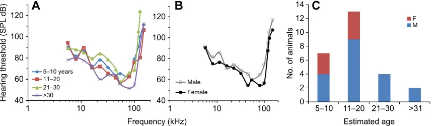
Audiograms from animals of the four age groups sampled
(5–10, 11–20, 21–30 and >30 years) overlapped substantially,
suggesting perhaps a slight but not obvious effect of age on the audiogram shape (Fig. 3A). However, there was a difference in threshold based on sex (Fig. 3B). The median male threshold was statistically higher than that of females across all frequencies (77
versus 72 dB, respectively; Mann–Whitney test, P<0.0001).
Males also showed more variability in their thresholds, with interquartile ranges (IQRs) and standard deviations of 13.6 and 10.5 dB, respectively; female IQRs and standard deviations were 9.6 and 9.3 dB, respectively. Overall, the sex ratio was skewed towards males, as many of the females observed were with a calf and were thus not captured.
The individual and mean (±s.d.) audiograms were plotted to further address population level audiograms and variability. There was a high degree of overlap between most audiograms with few, if any, being visually different (Fig. 4A). To better assess the difference between the greatest and least sensitive thresholds measured, the maximum and minimum thresholds at each frequency were plotted as two composite audiograms (Fig. 5A). This minimum threshold was a way to summarize the most sensitive thresholds we found. On average, the difference between these thresholds was 42 dB (mean), but was as small as 30 dB (5.6 kHz) and as large as 69 dB (100 kHz). Generally, the
maximum−minimum difference values were smallest (<35 dB) at
lower frequencies (≤16 kHz), reflecting that animals had generally
similar thresholds (and perhaps less hearing loss) in this low-frequency range. This difference tended to increase as test low-frequency increased (Fig. 5B) in a predictable and somewhat strong relationship
(y=8.95lnx+13.76;r²=0.73). The greatest differences (>50 dB) were
found at the‘best’hearing frequencies, where the lowest thresholds
tended to occur (54, 80 and 100 kHz), and at higher frequencies (128 kHz) where hearing abilities tended to cut off. Similarly,
40 60 80 100 120
1 10 100
5–10 years 11–20 21–30 >30
40 60 80 100 120
1 10 100
Male
Female
0 2 4 6 8 10 12 14
F M
Frequency (kHz)
Hearing threshold
(SPL
dB)
A
B
Estimated age
No. of
animals
[image:7.612.56.295.59.250.2]5–10 11–20 21–30 >31
C
Fig. 3. Categorical plots of hearing thresholds and demographics of 26 beluga whales sampled in Bristol Bay.(A,B) Audiograms categorized by (A) estimated age and (B) sex. SPL, sound pressure level. (C) Age and sex of belugas sampled.
0 5 10 15 20 25 30
Time (ms)
0.5
µ
V
Blank 117 dB
107
97
77
57
[image:7.612.93.524.587.712.2]47
Fig. 2. Example auditory evoked potential waveforms of a beluga whale.
The animal (ID: DlBB16-02) was recorded on 13 May 2016 and was the second animal of that field trip. Reponses are to 80 kHz, and decrease from 117 to 107, 97, 77, 57 and 47 dB, with the bottom trace being a‘blank’example, recorded without sound stimuli. Acoustic sinusoidally amplitude-modulated (SAM) stimuli start at 0 ms.
Journal
of
Experimental
variability in thresholds increased with frequency, with standard deviations increasing exponentially in a predictable, strong pattern
(y=8.5e0.004x;r²=0.80), reflecting greater variability at regions with
greatest sensitivity and at the highest frequencies (Fig. 5C). The ambient noise measurements showed that the background noise levels of the region were generally low. The 2012 measurements, taken over ca. 2 weeks but near the town of Dillingham, showed higher PSD sound levels at lower frequencies.
For example, at 1 kHz, background noise was 80 dB re. 1 μPa2Hz−1;
unfortunately, hearing with AEPs cannot be adequately tested at such low frequencies. At 5.6 kHz, the lower end of the audiogram frequencies tested, ambient noise levels were similar, about 80 dB re.
1 μPa2Hz−1. Ambient noise values tended to decrease with higher
frequencies. The 2016 mean PSD showed some overlap with the
lowest thresholds at 40–50 kHz, suggesting that masking may occur
in some instances in Bristol Bay. However, noise levels still fell below most hearing abilities of the animals tested, and these levels dropped substantially near 60 kHz, suggesting that sound levels of Bristol Bay were very low at higher (unmeasured) frequencies. Both sets of ambient noise PSD levels were about 20 dB below the mean hearing threshold and were also below the standard deviations of the population level audiograms (Fig. 4B).
We used the most sensitive values obtained from the sampled group (Fig. 5A) for measuring hearing loss in our sampled animals. The mean hearing loss across all animals increased logarithmically as
hearing test frequency increased (y=4.73lnx+6.63;r²=0.76; Fig. 6A).
Mean hearing loss values were generally lower at 4–16 kHz
(14–16 dB) but with some variability, i.e. the positive correlation
between frequency and average hearing loss was not clear at this
point. The amount of hearing loss was substantially higher (25–30 dB
mean) at higher frequencies (45–150 kHz), which supported the
positive correlation of frequency and average hearing loss.
The proportion of individuals with hearing loss, per category, differed for each frequency (Fig. 6B), but it was notable that as test frequency increased, the proportion of normal hearing thresholds decreased (Fig. 6B). This decrease in normal hearing at higher frequencies was further illustrated by the number of normal hearing thresholds. The number of normal hearing thresholds was negatively, albeit weakly, correlated with hearing test frequency
(r2=0.27; Fig. 6C). All other categories of hearing loss increased in
number with test frequency. The strength of these trends varied,
with a relatively poor correlation for slight hearing loss (r2=0.06),
but stronger relationships with frequency for mild (r2=0.54) and
moderate (r2=0.90) hearing loss categories.
Moderately severe was the highest category of hearing loss
observed in this study. Three belugas (DlBB_2012_07,
DlBB_2014_02, DlBB_2016_03) exhibited moderately severe hearing loss, all at the same frequency (100 kHz) in their audiograms (Fig. 7A). Although the moderately severe hearing loss was only noted at one frequency, the hearing sensitivity of these animals was generally not as good as that of the normal hearing animals, with only some small overlap at the lower frequencies. When comparing the median audiograms of all animals with normal, slight and mild hearing losses, it was possible to observe the relative scale of the upward trend of increasing thresholds (and thus loss of hearing sensitivity; Fig. 7B). However, there was some
7 8 9 10 11 12 13 14 15
1 10 100
20 40 60 80 100 120 140
1 10 100
Hearing threshold
(dB)
A
B
Max.–min. dif
ference
(dB)
s.d. of thresholds
(dB)
C
Frequency (kHz) 20
30 40 50 60 70 80
[image:8.612.49.467.58.221.2]1 10 100
Fig. 5. Evaluating hearing threshold differences.(A) Audiograms representing the highest thresholds (i.e. the poorest sensitivity; gray) and the lowest thresholds (i.e. greatest sensitivity; black) from 26 beluga whales sampled in Bristol Bay. (B) Difference between the maximum and minimum thresholds (dB re. 1 μPa) for each hearing test frequency. The maximum−minimum difference increased with frequency in a logarithmic fashion (y=8.95lnx+13.76;r²=0.73). (C) Standard deviation of the thresholds relative to the frequencies tested. This variation increased exponentially with frequency (y=8.51e0.0043x;r²=0.79).
20 40 60 80 100 120 140
1 10 100
20 40 60 80 100 120 140
1 10 100
Frequency (kHz)
Hearing threshold
(dB
re. 1
µ
Pa)
A
B
2012
2016
Ambient noise
(dB re.
1
µ
Pa
2 Hz
–1
[image:8.612.76.533.563.692.2])
Fig. 4. All audiograms and mean audiogram of all animals.
(A) Audiograms of all 26 animals examined during the 2012, 2014 and 2016 study periods (gray lines). Mean level of ambient noise for multiple sites (blue line; recorded in 2016) and ambient noise from longer-term measurements made in 2012 (black line) are shown. (B) Mean (±s.d.) audiogram of all animals examined (black circles) plotted with both noise measurements. Noise measurements are plotted in power spectral density (PSD: dB re. 1μPa2Hz−1).
Journal
of
Experimental
overlap in the mean hearing thresholds for these categories, reflecting that hearing thresholds varied within individuals and by hearing test frequency.
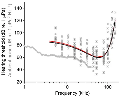
We developed an alternative to the mean and median methods often used to present multiple odontocete audiograms, because they are often affected by individual variability. To reduce this individual influence and provide a summary of all thresholds measured, we plotted a beluga composite audiogram using a fitted regression polynomial algorithm similar to that of Castellote et al. (2014) (Fig. 8). Such a method
provided a reasonably smooth fit to all the data (y=0.008x2−0.94x+
88.42;r²=0.57). In comparison, we used a least squares fit model for
the median audiogram (Branstetter et al., 2017). The two methods provided very similar population audiogram curves, without the
up–down scatter seen in the median and mean curves alone.
DISCUSSION
Understanding odontocete hearing sensitivity and the variability in hearing abilities at the population level is critical for evaluating noise exposure to the auditory system and to predict its behavioral effects. Overall, most beluga whales from the Bristol Bay population had
sensitive hearing (<80 dB) in the frequency range 16–100 kHz. The
lowest thresholds were from 45 to 80 kHz. Higher frequency hearing
abilities often extended to 80–100 kHz and these thresholds were
often low; multiple animals could hear up to 150 kHz. More than half (15 of 26) of those tested did not hear up to 150 kHz, indicating some high-frequency hearing loss. The most sensitive thresholds paralleled the relatively quiet ambient noise measurements.
These data and the thresholds of sensitive individuals were comparable to those of some odontocetes that were measured in controlled laboratory conditions and were without hearing loss. For example, the first and defining audiogram of a bottlenose dolphin
showed lowest thresholds (ca. 40–50 dB) from about 20 to 80 kHz,
and a high-frequency hearing limit near 150 kHz (Johnson, 1966).
A young Risso’s dolphin (Grampus griseus) showed lowest
thresholds from 22 to 90 kHz, with thresholds below 80 dB in a
wider range (8–110 kHz) than the belugas in the present study, and
upper hearing limits at 150 kHz (Nachtigall et al., 2005). Harbor
porpoises (Phocoena phocoena) may be more sensitive; one animal
showed thresholds below 40 dB from 32 to 140 kHz and a
high-frequency cut-off around 160–180 kHz (Kastelein et al., 2002).
White et al. (1978) measured two belugas; their best hearing was at 30 kHz (39 dB), average thresholds were below 50 dB from 30 to 80 kHz, below 80 dB from 5 to 120 kHz, and they demonstrated a
high-frequency limit near 130 kHz. Notably, the Risso’s dolphin
was also measured using AEPs (like these belugas), but the
porpoise, beluga and bottlenose dolphin were measured
behaviorally, a method that often demonstrates greater sensitivity (Yuen et al., 2005). Yet, many of the animals measured here had thresholds that were not vastly different from those of animals in controlled laboratory studies or from thresholds measured using
20 40 60 80 100 120 140
1 10 100
Frequency (kHz)
Hearing threshold
(SPL
dB)
A
B
20 40 60 80 100 120 140
1 10 100
Normal Slight Mild Normal
[image:9.612.56.298.57.432.2]Moderately severe
Fig. 7. Select individual and categorized audiograms with respect to hearing loss.(A) Beluga whales with moderately severe hearing loss for at least one frequency (black lines) and belugas with normal hearing (gray lines). (B) Median hearing thresholds for beluga whales with normal hearing, and slight or mild hearing loss. SPL in dBrmsre. 1 μPa.
0 5 10 15 20 25 30 35
0 20 40 60 80 100 120 140 160
Amount of hearing
loss (dB)
0 0.2 0.4 0.6 0.8 1.0
4 5.6 8 11.2 16 22.5 32 45 54 80 100 128 150
Moderately severe Moderate Mild Slight Normal
0 2 4 6 8 10 12 14
1 10 100
Frequency (kHz)
Rel. proportion of
hearing loss
groups
No. per hearing
loss group
A
B
C
Normal
Slight
Mild
[image:9.612.48.380.599.735.2]Moderate
Fig. 6. Hearing loss.(A) The average hearing loss per frequency (dB re. 1 μPa) for 26 beluga whales tested in Bristol Bay increased logarithmically as frequency increased (y=4.73lnx+6.23;r²=0.76). (B) Relative proportion of hearing loss for all individuals at frequencies measured was categorized as normal, slight, mild, moderate and moderately severe following Clark (1981). (C) Regressions of absolute numbers of individuals with hearing loss for all individuals across the frequencies measured. Ther2values for normal hearing
and slight, mild and moderate hearing loss were 0.27, 0.06, 0.54 and 0.90, respectively.
Journal
of
Experimental
more sensitive methods, indicating that these rapid, field-based AEP methods are truly able to acquire comparable auditory sensitivity data in additional wild populations.
One reason for the generally sensitive hearing thresholds may be partly related to the natural soundscape of Bristol Bay. Noise levels
(averaged over a multiday period) were as low as 40–50 dB re.
1μPa2Hz−1in some of the most sensitive hearing frequencies of the
belugas. The relatively low baseline noise would allow relatively sensitive hearing. Ambient noise, however, could be much higher during times we did not sample, such as during June and July when
the largest red salmon (Onchorynchus nerka) fishery in the world is
conducted. Thus, there is substantially increased boat traffic and concurrent vessel noise during this time. However, the peak fishing period is of relatively short duration, and open fishing times are often intermittent (dependent on rates of fish passage), suggesting that noise exposures and hearing impacts are potentially high amplitude but also short in duration. Further, boat noise tends to have dominant sound levels at lower frequencies (<5 kHz) (Kaplan and Mooney, 2015), less than the frequencies tested in this study, and in a range where belugas are not typically sensitive. Vessel noise has relatively little energy in the ultrasonic frequencies of best hearing for these belugas. We did not see frequent evidence of hearing loss; therefore, it is unlikely that vessel noise from fishing boats caused permanent hearing loss (threshold shifts) in these belugas. Of course, we do not know this for certain, and some hearing loss noted here could be noise induced. Small boat noise can have some energy at higher frequencies within the odontocete hearing range (Li et al., 2015) and this vessel noise could also potentially mask hearing thresholds. Unfortunately, this was not tested here.
Background noise levels would also be influenced by location, wind, tides and other factors in the bay. Although soundscapes could be quiet, we noted some ambient noise variability here (Fig. 4; see also Mooney et al., 2018). Yet, the most sensitive beluga hearing thresholds were similar to the low levels of ambient noise present.
Mean noise level values (in PSD) were 20–40 dB lower than the
average beluga audiogram, reflecting that thresholds were low (sensitive), perhaps enabling belugas to hear the full dynamic range (and thus low-amplitude cues) within an often (but not always) quiet environment. One challenge for such a comparison is that there are
only a few studies on beluga critical ratios (thus a limited sample size of animals and varied methods), and the bandwidth of the measured beluga auditory filters found in those studies varies (Johnson et al., 1989; Klishin et al., 2000; Finneran et al., 2002). Thus, a more detailed study of soundscapes and beluga auditory filters is needed to better evaluate the potential or likelihood of environmental masking. Notably, evoked potential thresholds are often several decibels higher than those measured in conditioned behavioral tasks (Yuen et al., 2005), suggesting that if these hearing thresholds could have been measured behaviorally, thresholds might be slightly lower. Together, these data reflect that the belugas in the present study often have sensitive hearing and are in a quiet environment, leading to the suggestion that that low environmental ambient noise may enable sensitive hearing thresholds. By extension, we would expect elevated hearing thresholds (i.e. less-sensitive hearing) in odontocetes from areas with greater ambient noise (e.g. high concentrations of snapping shrimp or nearby vessel traffic). However, we have measured only one population here; more studies of wild cetaceans, additional populations and their soundscapes could help test this idea.
To place these data in context, the thresholds were compared with those from several earlier studies that evaluated populations of odontocetes (Houser and Finneran, 2006b; Popov et al., 2007; Mann et al., 2010; Castellote et al., 2014). These comparisons should be taken with the consideration that the various studies used somewhat different methods, including differently constructed jawphones (or free-field transducers), jawphone placements, calibration distances and threshold estimation procedures, but this is all we have at this time. The median audiogram of all 26 animals measured here (±25th and 75th IQRs) closely overlapped with the audiograms of multiple belugas from laboratory or public display settings (Fig. 9A; Awbrey et al., 1988; White et al., 1978; Finneran et al., 2005; Klishin et al., 2000; Mooney et al., 2008). The median audiogram measured here was generally lower than the mean bottlenose dolphin audiograms in a population data set segregated by age (Fig. 9B). However, there was some overlap at the lowest frequencies (for most bottlenose dolphin age groups), and the youngest dolphin age group showed slightly greater sensitivity at frequencies >100 kHz. When compared individually with our beluga audiograms, there was substantially more overlap between bottlenose dolphin and beluga thresholds, for more age-related bottlenose dolphin groups (Fig. 9D). This beluga spread also overlapped with the audiogram of one rough-toothed dolphin, but was much lower than that of a second animal that had apparent hearing loss (Fig. 9C). The beluga thresholds measured here were generally quite similar to those of bottlenose dolphins measured by Popov et al. (2007), although their work showed a greater proportion of animals hearing up to 150 kHz. These dolphins were also wild caught, although they were housed in captivity for several months before testing. Although Popov et al. (2007) measured relatively young animals, the animals showed a slight increase in hearing thresholds and cut-off frequency with age, suggesting some mild age-related hearing loss, perhaps more so than noted here. However, it is not certain how Popov et al. (2007) determined age; the beluga age estimator method we used is based on length and, although not specific to Bristol Bay, it is likely a rough estimate of age.
Our finding of a relatively low prevalence of hearing loss in Bristol Bay belugas is quite different from that in some populations of stranded animals, where substantial hearing loss occurred in 60% of animals tested (Mann et al., 2010). When considering the maximum amount of hearing loss for an animal, we found that only 3 of 26 (ca. 12%) showed moderately severe hearing loss at one frequency. Similarly, 3 showed slight hearing loss, 13 (50%)
20 40 60 80 100 120 140
1 10 100
Frequency (kHz)
Hearing threshold
(dB
re. 1
µ
Pa)
Ambient noise
(dB re.
1
µ
Pa
2 Hz
–1
[image:10.612.70.274.55.221.2])
Fig. 8. Modeled population audiogram.Hearing thresholds for all 26 animals, all frequencies, and modeled hearing thresholds using a custom least squares fit algorithm (black;y=0.008x2−0.94x+88.42;r²=0.57), modified from
Castellote et al., 2014, whereyis the threshold andxis the frequency. A similar least squares fit model for the median audiogram (following Branstetter et al., 2017) is shown in red. Data are relative to the average noise floor of Bristol Bay (stationary 2012 site; gray line), plotted in PSD (dB re. 1μPa2Hz−1).
Journal
of
Experimental
showed mild hearing loss and 7 (27%) showed moderate hearing loss. When averaging the amount of hearing loss for each animal across all its tested frequencies, we found that animals had relatively good hearing overall: 8 showed normal hearing (30%), 9 (35%) showed slight hearing loss and 9 showed mild hearing loss. Of course, how we quantify hearing loss matters. Following previous studies, we quantified hearing loss as the difference from the most sensitive values obtained from the sampled group (Fig. 5A). But, notably,
‘normal’hearing was not expected to always reach those sensitive
hearing values; rather, there was a 15 dB range that encapsulated
animals which heard ‘normally’. All hearing loss categories were
defined by a range of sound levels (e.g. 0–15 dB). This method allows
variation, including natural biological and measurement differences, and thus would not lead to overestimating hearing loss cases. On average, for this subset of the Bristol Bay beluga population, hearing loss fell in the normal, mild and slight range, suggesting that animals often had sensitive hearing. When hearing loss was split by frequency and animal, greater incidences of more substantial hearing loss were noted. Perhaps this hearing variation within presumably healthy
belugas is a better representative of the‘natural’variation in wild
populations than we have previously been able to sample.
One question that is important to address is: are these trends in variability and proportions of hearing loss what we would expect? Humans and bottlenose dolphins offer some comparison. Humans and dolphins in human care show greater variability in sensitivities and more hearing loss (Cruickshanks et al., 1998; Houser and Finneran, 2006b). It is possible that we did not sample the older segment of this population adequately as our sample animals were potentially younger than the overall population and thus we would have failed to document the natural population rate of age-related hearing loss that is seen in bottlenose dolphins and humans (Cruickshanks et al., 1998; Houser and Finneran, 2006b). Apart from age, aminoglycosides or other ototoxic drugs and conditions of living may influence variability as well. Additionally, belugas with poor hearing abilities may be subject to greater selection pressures (Mann et al., 2010; but see Ridgway and Carder, 1997). Notably, the variability seen here was relatively small, with standard deviations between 8 and 16 dB SPL. This is lower than that of some other
dolphin populations (Houser and Finneran, 2006b; Popov et al., 2007), although this variability tends to be frequency dependent. Of course, some variability in our (and these aforementioned) studies may be test/re-test methodological variability. We were not permitted to recapture wild animals, so our re-test variability remains unknown. Perhaps there is some natural selection against animals with hearing loss (or a correlation with other health parameters which are related to poor survival). This concept would suggest that we
should be cautious when evaluating a species’hearing abilities based
upon stranded, often sick, animals. Further, there could be changes between populations on longer, evolutionary timescales. It should be noted that the audiograms measured here closely overlapped with those of many belugas in zoological facilities. This similarity between captive and wild animals supports not only the fidelity of the two populations and applications of their respective data sets but also the robustness of the data set collected here.
Beyond our study, and those odontocete studies mentioned above, we know of no audiogram field measurements in healthy wild mammal populations to offer a comparison with these data or place our measured variability in context. Studies of fish might offer an option, but their hearing mechanisms are so different that we suggest this is not viable (Amoser and Ladich, 2005; Popper and Fay, 2011). Thus, we do not really know what to expect with regards to hearing variability and proportions of natural hearing loss. Rather, these data provide the baseline to evaluate what the proportions of hearing loss may be in other healthy mammal populations in relatively pristine environments.
Additional studies are needed to quantify the hearing of a greater proportion (demographically) of this Bristol Bay population as well as the hearing of additional populations in both quiet and noisy environments (e.g. Cook Inlet, AK, USA, and St Lawrence Estuary, Canada) where chronic noise is suspected to be a stressor for these small populations (Blackwell and Greene, 2002). Here, we found generally good hearing (mostly normal and slight incidences of hearing loss). There is a need to address the hearing of animals in habitats with greater noise levels. Their proportions of hearing loss will reveal a great deal about how noise levels impact wild odontocete hearing. The fact that we were able to detect hearing loss
30 50 70 90 110 130 150
1 10 100
30 50 70 90 110 130 150
1 10 100
30 50 70 90 110 130 150
1 10 100
0–9 years 10–19 20–24 25–29 30–39 40–49 Median 1st quartile 3rd quartile 30
50 70 90 110 130 150 170
0.1 1 10 100
A
B
C
D
Hearing threshold
(dB)
Frequency (kHz)
Fig. 9. Comparison of audiograms from Bristol Bay belugas with those measured in previous studies.(A) Median threshold (black circles) of all beluga whales measured in this study (n=26) with ±25th and 75th interquartile ranges (IQR, upper and lower solid black lines) plotted with thresholds from belugas measured in laboratory settings (red lines; see Discussion for references). (B) Median thresholds ±25th and 75th IQR of the 26 beluga whales (black circles and black lines) measured in this study compared with those of captive bottlenose dolphins by age class (red lines; adapted from Houser et al., 2008). (C) Audiograms of all belugas from this study plotted (grayscale) with audiograms from two stranded bottlenose dolphins (red lines). One dolphin (Castaway; open red squares) shows hearing loss; the other dolphin is a calf (Ginger; filled red triangles) with presumably‘normal’hearing (adapted from Mann et al., 2010). (D) Beluga audiograms from this study (grayscale) compared with the bottlenose dolphin audiograms combined by age class in B, showing that thresholds of individuals overlapped with most of the mean thresholds of most bottlenose dolphin age groups.
Journal
of
Experimental
in wild belugas means that they survive with this impairment at least in the Bristol Bay population. Low proportions of hearing loss could also mean that most do not survive and that levels of noise that cause hearing loss may have severe impacts on individual health and survival and on population abundance. Noise is also increasing across much of the Arctic. If other beluga populations prove to have similarly sensitive hearing, there should be substantial concern that noise produced by humans, from the many, varied noise sources, may affect the auditory system and perhaps health of these marine mammals.
We incorporated additional ways to quantify hearing variability beyond simple mean audiograms, as the mean can be highly influenced by variability and outliers. Median and population best-fit polynomials not only best-fit the data better but also offer a more parsimonious way to evaluate the data. Additionally, by developing a maximum sensitivity audiogram for this population, we provided a way to quantify the amount of hearing loss. This lower threshold audiogram also demonstrates the range of sensitivity and enables a more cautious approach to address the sound levels that may impact hearing.
Understanding the natural variation in hearing abilities of a wild species or population expands our capacity to potentially distinguish between hearing loss caused by anthropogenic noise and loss as a result of age or other natural factors. Variability in hearing sensitivity and thresholds can be used to determine whether man-made noise affects the hearing ability of a population. Further, understanding population level hearing sensitivity and variability
facilitates the estimation of noise-related harassment or ‘take’
events. Additionally, understanding hearing sensitivity, variability and subsequent impairments may help diagnoses of stranded animals. Hearing remains the most important sensory modality for odontocetes, enabling acoustic communication and echolocation. Thus, understanding how well an animal hears relative to other members of its population aids evaluation of overall health and considerations of release in stranded animals.
In conclusion, these data provide an initial population level audiogram for Bristol Bay belugas [26 of ca. 2000 animals (Allen and Angliss, 2012; Citta et al., 2018)] and are the first population-subset audiograms for a healthy wild odontocete population. Animals overall showed sensitive hearing, with average hearing thresholds not exceeding mild hearing loss; this sensitivity is perhaps indicative of a relatively quiet habitat. Although measuring auditory neurophysiology in the field was no easy task, especially in extreme environments such as the marine high latitudes, the low physiological noise levels of the data and successful records on all animals tested reflect the success of this method. To place these data in a broader context, we suggest collecting audiograms from more individuals of this population, from individuals in other beluga populations (in quiet and noisy environments) and from individuals of other cetacean species. Beyond marine mammals, the sensitivity and apparently low variability of auditory thresholds noted here provide a baseline to establish and compare sound sensitivities in many other taxa, an increasingly vital task as anthropogenic noise encroaches more and more on animal habitats.
Acknowledgements
We acknowledge substantial assistance in data collection from Russ Andrews, Dennis Christen, George Biedenbach, Brett Long, Stephanie Norman, Mandy Keogh, Amanda Moors, Jennifer Trevillian, Laura Thompson, Tim Binder, Lisa Naples, Leslie Cornick, Katie Royer, William Hurley III, Justin Richards, Natalie Rouse, Renae Sattler and Kathy Burek-Huntington. Local support in Bristol Bay was substantial and included an experienced beluga capture team including Ben Tinker, Richard and Joe Hiratsuka, Albie Roehl, William and Daniel Savo, and Danny
Togiak. We also thank their respective first mates and shore support provided by Helen Aderman. Paul Nachtigall and Alexander Supin assisted with the auditory evoked potential program. Thank you to the Mooney Lab (WHOI), including Ian Jones and Tammy Silva for help with figures.
Competing interests
The authors declare no competing or financial interests.
Author contributions
Conceptualization: T.A.M., M.C., R.H., C.G.; Methodology: T.A.M., M.C., L.Q., R.H., C.G.; Formal analysis: T.A.M., M.C.; Investigation: T.A.M., M.C., L.Q., R.H., E.G., C.G.; Resources: T.A.M., M.C., C.G.; Data curation: T.A.M., M.C.; Writing - original draft: T.A.M.; Writing - review & editing: T.A.M., M.C., L.Q., E.G., C.G.; Project administration: C.G., L.Q., M.C.; Funding acquisition: T.A.M., M.C., C.G.
Funding
Project funding and field support were provided by multiple institutions, including Georgia Aquarium, the Marine Mammal Laboratory of the Alaska Fisheries Science Center (MML/AFSC), and the Woods Hole Oceanographic Institution (Arctic Research Initiative, Ocean Life Institute and Marine Mammal Center). Field work was also supported by National Marine Fisheries Service Alaska Regional Office (NMFS AKR), U.S. Fish and Wildlife Service, Bristol Bay Native Association and Bristol Bay Marine Mammal Council, Alaska SeaLife Center, Shedd Aquarium and Mystic Aquarium. Audiogram analyses were initially funded by the Office of Naval Research award number N000141210203.
References
Allen, B. M. and Angliss, R. P.(2012). Beluga whale (Delphinapterus leucas): Cook Inlet stock.Alaska Marine Mammal Stock Assessments NOAA-TM-AFSC-245.
Amoser, S. and Ladich, F.(2005). Are hearing sensitivities of freshwater fish adapted to the ambient noise in their habitats?J. Exp. Biol.208, 3533-3542. ANSI(1951).Specifications for Audiometers for General Diagnostic Purposes.
Z24.5, New York: American National Standards Institute. Au, W. W. L.(1993).The Sonar of Dolphins. New York: Springer.
Au, W. W. L.(2000). Hearing in whales and dolphins: an overview. InHearing by Whales and Dolphins(ed. W. W. L. Au, R. R. Fay and A. N. Popper). New York: Springer-Verlag, Inc.
Au, W. W. L. and Hastings, M. C.(2009).Principles of Marine Bioacoustics. New York: Springer.
Au, W. W. L., Popper, A. N. and Fay, R. J.(2000).Hearing by Whales and Dolphins, p. 512. New York: Springer-Verlag.
Awbrey, F. T., Thomas, J. A. and Kastelein, R. A. (1988). Low-frequency underwater hearing sensitivity in belugas,Delphinapterus leucas.J. Acoust. Soc. Am.84, 2273-2275.
Beauregard-Tellier, F. (2008). The Arctic: Hydrocarbon Resources. Ottawa, Canada: Parlamientary Information and Research Service, Library of Parliament. Blackwell, S. B. and Greene, C. R.(2002). Acoustic measurements in Cook Inlet,
Alaska, during August 2001: Greeneridge Sciences, Incorporated.
Branstetter, B. K., St. Leger, J., Acton, D., Stewart, J., Houser, D., Finneran, J. J. and Jenkins, K.(2017). Killer whale (Orcinus orca) behavioral audiograms.
J. Acoust. Soc. Am.141, 2387-2398.
Castellote, M., Mooney, T. A., Hobbs, R., Quakenbush, L., Goertz, C. and Gaglione, E.(2014). Baseline hearing abilities and variability in wild beluga whales (Delphinapterus leucas).J. Exp. Biol.217, 1682-1691.
Citta, J. J., Quakenbush, L. T., Frost, K. J., Lowry, L., Hobbs, R. C. and Aderman, H.(2016). Movements of beluga whales (Delphinapterus leucas) in Bristol Bay, Alaska.Mar. Mamm. Sci.32, 1272-1298.
Citta, J. J., O’Corry-Crowe, G., Quakenbush, L. T., A. L. Bryan, Ferrer, T. and Olson, M. J.(2018). Assessing the abundance of Bristol Bay belugas with genetic mark-recapture methods.Mar. Mamm. Sci.
Clark, J. G.(1981). Uses and abuses of hearing loss classification. Asha23, 493-500.
Cook, M. L. H. and Mann, D. A.(2004). Auditory brainstem response hearing measurements in free-ranging bottlenose dolphins (Tursiops truncatus).
J. Acoust. Soc. Am.116, 2504.
Cook, M. L. H., Verela, R. A., Goldstein, J. D., McCulloch, S. D., Bossart, G. D., Finneran, J. J., Houser, D. S. and Mann, D. A.(2006). Beaked whale auditory evoked potential hearing measurements.J. Comp. Physiol. A.192, 489-495. Cornick, L. A., Quakenbush, L. T., Norman, S. A., Pasi, C., Maslyk, P., Burek,
K. A., Goertz, C. E. and Hobbs, R. C.(2016). Seasonal and developmental differences in blubber stores of beluga whales in Bristol Bay, Alaska using high-resolution ultrasound.J. Mammal.97, 1238-1248.
Cruickshanks, K. J., Wiley, T. L., Tweed, T. S., Klein, B. E. K., Klein, R., Mares-Perlman, J. A. and Nondahl, D. M.(1998). Prevalence of hearing loss in older adults in Beaver Dam, Wisconsin the epidemiology of hearing loss study.
Am. J. Epidemiol.148, 879-886.