On the Stabilization of Linear Time Invariant Systems with Positive Controls

U

niversity of

T

wente

A

pplied

M

athematics

C

hair of

H

ybrid

S

ystems

On the Stabilization of Linear Time Invariant

Systems with

POSITIVE CONTROLS

Author

F.L.H. Klein Schaarsberg

Supervisor Prof. Dr. A.A. Stoorvogel

GraduationCommittee Prof. Dr. A.A. Stoorvogel Prof. Dr. H.J. Zwart Dr. M. Schlottbom

P

reface

During the past seven months I have been working on this project with the objective of concluding my study in Applied Mathematics at the University of Twente. It closes off my almost six year time as a student at this university which I, after a difficult start, embraced as my home.

My time as a student overall has been the most enjoyable and memorable period of my life. I believe that I have developed myself academically, but more importantly that I developed myself to become the person that I am today. As excited as I am to move on to graduate life, I can not help but to think I will miss all of the things I have done and experienced in university. I have met some amazing people, made new friends with whom I have built many good memories, and I have done many things I am proud of, looking back.

I would like to take this opportunity to express my gratitude to a couple of people. First of all I would like to thank my parents for making it possible for me to study, and for supporting me in everything I did, even though sometimes they may have had no clue what that was exactly. Special thanks go to my brother for the momorable moments we shared in the past years, to Juliët for being there for me in all times, and to Sagy, David, Sander, Rico and Mike for their mental and social support.

S

ummary

This report studies the stabilization of control systems for which the control input has a positivity constraint, that is, one or more of the control inputs is either positive or zero. Typical examples of such systems are systems for which the control can only add (for example energy or substances), but cannotextract. A classic example is that of a heating system in buildings. Radiators can only release heat into the rooms, but it cannot extract the heat when the temperature overshoots the setpoint.

This report is build up out of three main parts. The first part concerns a review on mathematical research on systems with positive control, in particular forlinear time invariant

systems. Such systems may be represented by the state-space representation

˙

x= Ax+Bu,

with statexand control inputu. Two representative papers are studied in more detail. One approaches the positive control problem from the perspective ofoptimal control. The other investigates positive state feedback stabilization of linear time invariant systems with at most one pair of unstable complex conjugate poles. This latter paper forms the basis for this project.

The second and third part focus on linear time invariant systems in general. It extends known results to systems with more than one pair of unstable complex conjugate poles, where the positive control input is scalar. Two approaches are considered.

The first approach uses Lyapunov’s stability theory as a base for a asymptotically stabilizing positive control law. Formal proofs of stability are given for stable (but not asymptotically) oscillatory systems. The feasibility of the control law for unstable oscillatory systems is investigated through simulations.

C

ontents

Preface i

Summary iii

Contents v

Nomenclature vii

1 Introduction to the positive control problem 1

1.1 Structure or this report . . . 2

1.2 Preliminary definitions . . . 2

1.3 An illustrative example: the simple pendulum . . . 4

2 Overview of literature 7 2.1 Stabilizing positive control law via optimal control . . . 8

2.2 Positive state feedback for surge stabilization. . . 8

3 The four-dimensional problem 13 3.1 Brainstorm on approaches . . . 14

3.2 Motivation . . . 17

3.3 Formal problem statement. . . 17

4 Lyapunov approach 19 4.1 Lyapunov stability theory . . . 19

4.2 Control design for stable systems. . . 21

4.3 Unstable systems . . . 35

5 State feedback via singular perturbations 39 5.1 Theory of singular perturbations . . . 39

5.2 Application to the four-dimensional problem. . . 40

5.3 Application in simulations. . . 44

5.4 Concluding remarks . . . 47

6 Conclusion 51

7 Recommendations and discussion 53

8 Bibliography 55

A Simulations in Matlab A-1

B Auxiliary Theorems and Definitions B-2

C Alternative approach concerning Theorem 11 C-3

D Positive control problem approached from optimal control D-4

N

omenclature

The next list describes several symbols that will be later used throughout this thesis.

N The set of all natural numbers:N={0, 1, 2, 3, . . .} N>0 The set of all natural numbers except 0: N\ {0}

Z The set of all integers (whether positive, negative or zero):Z={. . . , 2, 1, 0, 1, 2, . . .} Q The set of all rational numbers:Q={a

b|a,b∈Z,b6=0}

R The set of all real numbers Rn _{Then-dimensional (n∈N}

+) real vector space over the field of real numbers

Rn×m _{The n×m-dimensional (n,m ∈ N}

+) real matrix space over the field of real

numbers

R≥0,R>0 The set of non-negative real numbersR≥0 ={µ∈R|µ≥0}, and

similarlyR>0={µ∈R|µ>0}

Rn

≥0 The nonnegative orphant inRn:Rn≥0 :={µ∈Rn|µi≥0}

ı Imaginary unitı:=√−1

C The set of all complex numbers:C={a+bı|a,b∈R}

t General variable for time

τ Alternative variable for time

t0 Starting time

tf Final time

T Fixed time span

T Fixed time span (alternative)

x(t) State vector inRn at timet

χ_{i(t) i}th_{entry ofx(t)}

x0 Initial statex0:=x(t0)

xf Final statexf =x(tf)

¯

x Equilibrium state inRn

˙

x(t) State vector time derivative of dimensionnat timet

θ(t) Angle in radians at timet

˙

θ(t), ¨θ(t) First and second time derivative ofθat timet

u(t) Control input vector of dimensionpat timet

A System matrix (A∈Rn×n₎

B Input matrix (B∈Rn×p₎

O_{A,C} The observability matrix of the pair(A,C), as defined inTheorem 2

V(x(t)) Lyapunov function ˙

V(x(t)) Derivative of Lyapunov function with respect to timet

Mt

Transpose of matrixM, also applies to vectors

rank(M) The rank of matrixM.

E_λ(M) The set of eigenvalues of matrixM

In×n Then×nidentity matrix. Then×nsubscript is sometimes omitted if the size

is evident

P,Q Positive definite matrices

Lp[a,b] The space of functions f(s)on the interval[a,b]for which

||f||_p =

Z b

a |f

(s)|pds < ∞. Commonly a = t0 and b = ∞ such that one

considersLp[t0,∞)

||·||_p Standard p-norm

h·,·i Inner product

lcm(a,b) The least common multiple of numbersaandb.

1.

I

ntroduction to the positive control problem

There are many real life examples of systems for which the control input is nonnegative, also known as one-sided. A typical example most people can relate to is that of heating systems in houses or other buildings. A central heating system essentially provides warmth to the interior of a building. A conventional system circulates hot water through radiators which release heat into rooms. These radiators are often equiped with thermostatically controlled valves. These valves can either be opened (fully or to some level) or be closed. Therefore the radiator can only release energy into the room (valve open), or add no energy at all (valve closed). It cannot extract heat from the room, and hence the heating system is categorized as a system with positive control.

Examples of positive control systems that are closely related to the central heating example are systems which involve flow of fluids or gasses that are controlled by one-way valves. Such systems occur for example in mechanics and chemistry. Consider for instance a chemical plant where several substances are to be added to a reaction vessel. Once added, substances mix and/or react to produce the desired end product, and hence the raw substances cannot be extracted individually anymore. Hence, ifui controls the addition of

substancei, then this is a positive control since extraction is not possible.

These control systems also occur in medical fields. For example in pumps that intravenously administer medication to a patient’s bloodstream. An artificial pancreas is an example of a positive control system since insulin can only be added to a patient’s body, and cannot be extracted via the pump. Many other control systems can be listed which can be categorized as positive control. For example economic systems with nonnegative investements, or in electrical networks with diode elements (which have low resistance in one direction and high, ideally infinite, resistance in the other). Also the classical cruise control is an example of positive control since the control system only operates the throttle and not the brakes.1

The control systems as described in the above examples are commonly represented by a system of differential equations. Stabilization of such systems has been studied extensively in the field of control theory. Consider the control system ofncoupled differential equations with pcontrol inputs given by

˙

x(t) = f(x(t),u(t),t). (1)

Herex(t)∈Rn_{denotes then-dimensionalstate vectorof the system at timet, its derivative}

with respect to time at timetis denoted by ˙x(t), which is also ann-dimensional column vector. At timetthecontrol(or input) vector is denoted byu(t)∈Rp_{. If the control restraint}

set is denoted byΩ⊆Rp_{, thenu :[t}

0,∞)→Ωfor some initial timet0. Note that there may be a final timetf <∞such thatu:[t0,tf]→Ω. In the most general case the control

input is unrestricted, in that caseΩ=Rp. Regularity conditions should be imposed on the function f :Rn →Rn _{to ensure that(1)has a unique solutionx(t),t≥t}

0, for every initial statex0∈Rnand every control inputu(t).

The control problem (1)is called apositive control problemif one of more of the control inputs are constrained to being nonnegative. In order to formally state the positive control problem, define

Rm

≥0 :={µ∈Rm|µi ≥0}.

as the nonnegative orphant inRm_{. The control problem(1)is said to be a positive control}

problem if there exists a nonempty subset of indices P ⊆ {1, 2, . . . ,p}of cardinalitym, 1≤m≤p, such that

uP[t0,∞)→Ω≥0,

1. INTRODUCTION TO THE POSITIVE CONTROL PROBLEM

whereΩ≥0is anmdimensional subspace ofR≥0m, that isΩ≥0⊆R≥0m. It is (often) assumed

that them-dimensional zero vector~0 is an element ofΩ≥0, so that the zero control is in the restraint setΩ≥0. In the least restrictive caseΩ≥0=Rm≥0.

The system (1) is the most general representation of a control system of differential equations. No assumptions concerning linearity of time invariancy are made there. Control problems are more than often concerned with linear time invariant (LTI) systems. In many cases non-linear systems are approximated by linear systems, as in the example of Section 1.3. As will be apparent in Section 2, most research into positive control systems concerns LTI systems. Hence, also this report focusses on the stabilization of linear time invariant (LTI) systems of differential equations using positive control. In that case Equation (1)is of the form

˙

x(t) =Ax(t) +Bu(t), x(t)∈Rn, u(t)∈Rp, (2)

where matricesA∈Rn×n _andB∈Rn×p_{are called thesystem matrixand theinput matrix}

respectively. In some instances the system’soutput vector y(t)∈Rq_{output is defined by}

y(t) =Cx(t) +Du(t), C∈Rq×n, D∈Rq×p, (3)

withoutput matrix Candfeedthrough matrixD.Equations (2)and(3)are called a ‘state-space representation’ for an LTI system.

1.1.

S

tructure or this report

The previous section aimed to introduce the concept of ‘positive control’. The report is structured as follows: The remainder of this chapter includes some preliminary definitions inSection 1.2followed the classic example of the simple pendulum with positive controls inSection 1.3. Section 2concerns a study into literature of mathematical research into systems with positive controls. That section includes a more detailed review of two notable works. The main problem that is considered in this report is introduced inSection 3. It includes a motivation for the two approaches individually described in the sections to follow.Section 4approaches the positive control problem from Lyapunov’s stability theory, Section 5approaches the problem with techniques of singular perturbations for ordinary differential equations. The report closes with a conclusion inSection 6and a discussion and recommendations inSection 7.

1.2.

P

reliminary definitions

This section aims to introduce some well know concepts that will be used in one way or another throughout this report. Consider the system ˙x = f(x), an equilibrium of such system is defined as follows:

Definition 1(Equilibrium) ¯x∈Rn_{is anequilibrium (point)of(12)if f(x¯) =0.}

An equilibrium point is also known as a ‘stationary point’, a ‘critical point’, a ‘singular point’, or a ‘rest state’. A basic result from linear algebra is that Ax=0 has only the trivial solutionx=0 if and only if Ais nonsingular (i.e. Ahas an inverse). So for LTI systems

˙

x= Ax, ¯x =0 is the only equilibrium if and only if Ais nonsingular. The aim of applying controluis to stabilize the system at ¯x =0. This means that ˙x=Ax+Bu=0 if and only of Ax = −Bu. Assuming that Ais non-singular one finds that 0 = x¯ = A−1_{Bu¯, which} implies that ¯u=0 if and only ifA−1_{Bis injective.}

Equilibria as defined inDefinition 1can be categorized as follows:

1. INTRODUCTION TO THE POSITIVE CONTROL PROBLEM

Definition 2(Stable and unstable equilibria) An equilibrium point ¯xis

1. stableif∀ε>0∃δ>0 such that||x0−x¯||<δimplies||x(t;x0)−x¯||<ε∀t>t0.

2. attractiveif∃δ1>0 such that||x0−x¯||<δ1implies that limt→∞x(t;x0) =x¯.

3. asymptotically stableif it is stable and attractive.

4. globally attractiveif limt→∞x(t;x0) =x¯for everyx0∈Rn.

5. globally asymptotically stableif it is stable and globally attractive.

6. unstableif ¯x is not stable. This means that∃ε>0 such that∀δ>0 there existx0and at1such that||x0−x¯||<δbut||x(t1;x0)−x¯|| ≥ε.

A similar categorization can be made for systems of the form ˙x =Ax. The poles of such system, given by the eigenvalues of the system matrixA, determine the categorization of stability of the system. If the poles of the system are given byEλ(A), then the system is

called

• stableif all poles have their real part smaller or equal to zero (in the case where the real part equals zero, then the imaginary part cannot equal zero);

• asymptotically stableif all poles have their real part strictly smaller than zero;

• unstableif one or more of the poles have real part greater than zero.

Systems for which poles have nonzero imaginary part are sometimes calledoscillatory. Note that thepolesof the system ˙x =Axare equal to theeigenvaluesof the matrixA. The terms ‘poles’ and ‘eigenvalues’ are used side by side. Note that systems with zero real part are

categorized as ‘stable’, but explicitly not ‘asymptotically’.

For state-space representation(2)and(3)representations the concepts ofcontrollabilityand

observabilityare introduced as follows.

Theorem 1 (Controllability matrix) Consider the system x˙ = Ax+Bu, with state vector x ∈ Rn×1_{, input vector u ∈ R}r×1_{, state matrix A ∈ R}n×n _{and input matrix B ∈ R}n×r_{. The}

n×nrcontrollability matrixif given by

C_{A,B}=hB AB A2B . . . An−1Bi. (4)

The system is controllable if the controllability matrix has full row rank, that isrank(C{A,B}) =n.

Roughly speaking, controllability describes the ability of an external input (the vector of control variablesu) to move the internal statex(t)of a system from any initial statex0to any other final statext_f in a finite time interval. More formally, the systemEquation (2)

is called controllable if, for eachx1, x2 ∈ Rn there exists a bounded admissible control

u(t)∈Ω, defined in some intervalt1≤t≤t2, which steersx1=x(t1)tox2=x(t2).

A slightly weaker notion than controllability is that of stabilizability. A system is said to be stabilizable when all uncontrollable state variables can be made to have stable dynamics.

Theorem 2(Observability matrix) Consider the systemx˙=Ax+Bu with output y=Cx+Du, with state vector x ∈ Rn×1_{, input vector u ∈ R}r×1_{, state matrix A ∈ R}n×n_{, input matrix}

1. INTRODUCTION TO THE POSITIVE CONTROL PROBLEM

matrixif given by

O{A,C}=



       

C CA CA2

.. . CAn−1



       

. (5)

The system is observable if the observability matrix has full column rank, that isrank(O{A,C}) =p.

Observability means that one can determine the behavior of the entire system from the system’s outputs.

Some of the literature ofSection 2use the concept oflocal null-controllability. A system is called locally null-controllable if there exists a neighbourhoodVof the origin such that every point ofVcan be steered tox=0 in finite time.

1.3.

A

n illustrative example

:

the simple pendulum

To illustrate the positive control problem, consider the specific case in which the positive control input is a linear state feedback. Consider the linear system (A,B) given by Equation (2). The state feedback control input is computed asu(t) = Fx(t) for some real matrixF ∈ R1×n _{such that the scalar positive control input is computed as u(t) =}

max{0,Fx(t)}.

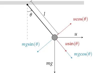
A classic and illustrative example is that of the so-called ‘simple pendulum’ as depicted in Figure 1. The rod of the pendulum has lengthl. At the end of the rod a weight of mass

mis attached, the rod itself is assumed to be weightless. The gravitational force on the weight is equal tomg, wheregis the gravitational constant. Its direction is parallel to the vertical axis. The angle between the pendulum and the vertical axis is denoted byθradians. Positive angle is defined as the pendulum being to the right of the center. A horizontal force of magnitudeucan be exerted on the weight. On the horizontal axis, denote positive forces as forces pointed to the right.

θ

mgcos(θ)

mgsin(θ)

mg

u ucos(θ)

usin(θ)

l

Figure 1: Simple pendulum of lengthl of massmwith gravitational forcemgand external horizontal forceu.

As inFigure 1, both forces can be decomposed into components in the direction of motion (perpendicular to the pendulum) and perpendicular to the direction of motion. The former are the forces of interest, since the latter forces are cancelled by an opposite force exerted by the rod. The netto force on the mass in the direction of movement is equal to

1. INTRODUCTION TO THE POSITIVE CONTROL PROBLEM

ucos(θ) +mgsin(θ). The equation of motion for a pendulum with friction coefficientkis given by

mlθ¨+klθ˙+mgsin(θ) +ucos(θ) =0.

Equivalently, one can write

¨ θ=−k

mx2− g

lsin(x1) +

1

mlucos(x1).

Now define statesx1 :=θ andx2 :=θ. That way the system of differential equations is˙ obtained described by

˙

x1=x2

˙

x2=−

k mθ˙−

g

lsin(θ)−

1

mlucos(θ).

(6)

This model obviously is non-linear. The equilibrium of interest isx=h0 0i t

,u=0, where the pendulum hangs vertically. When the system is linearized around this equilibrium the following linear state-space matrices are acquired:

A=

"

0 1

−g_lcos(x1)−ml1usin(x1) −mk

# _x=~₀

u=0 =

"

0 1

−g_l −k m

#

, B=

" 0

−1

mlcos(x1) #

_x=~₀

u=0 = " 0 −1 ml # .

That way the systemEquation (6)linearized aroundx=h0 0i t

,u=0 is given by

˙

x =

"

0 1

−g_l −k m # x+ " 0 − 1 ml # u

For now, consider a frictionless pendulum, sok=0. Let for this pendulum also g_l =1 and

m= 1_l. The linearized system is then described by

˙ x= " 0 1 −1 0 #

| {z }

A x+ " 0 −1 #

| {z }

B

u.

A close inspection of Areveals that its eigenvalues are equal to±ı, which indeed illustrates the frictionless property of the pendulum. Let the control input be defined as a stabilizing state feedback controlu=Fx, which is proportional with the direction and angular speed of motionx2. For this example let F =

h

0 1i. It can be verified that the eigenvalues of

(A+BF) are equal to −1 2±12

√

3ı, and hence have strictly negative real part such that the controlled system ˙x(t) = (A+BF)x(t)is stable. Vice versa, given the desired poles of(A+BF), the feedback matrixFcan for example be computed via Ackermann’s pole placement formula, seeTheorem B.1.

1. INTRODUCTION TO THE POSITIVE CONTROL PROBLEM

0 5 10 15 20 25

-2 0 2 4

x1 x2

0 5 10 15 20 25

time (t) -2

-1 0 1

u

Figure 2: Simulation of a single simple pen-dulum with regular state feedback control

u(t).

0 5 10 15 20 25

-4 -2 0 2 4

x1 x2

0 5 10 15 20 25

time (t) 0

0.5 1 1.5 2

u

Figure 3: Simulation of single simple pen-dulum with positive state feedback control

˜

u(t).

˜

ubecomes positive again. Therefore, one would expect that also ˜ustabilizes the system, but slower thanudoes. This intuition is supported by a simulation of both systems. The results are included inFigure 2for the regular controlu, and inFigure 3for the pendulum with positive control ˜u.

In this example a hanging frictionless pendulum was stabilized, which is a stable system by itself (not asymptotically stable). For this system the positive state feedback control law worked in order to stabilize the system. For unstable systems, this may be a different story. Consider for example a pendulum that is supposed to be stabilized around its vertical upright position, where the positive control can only push the pendulum one way. It is a known result that (a well designed) ‘regular’ state feedback control can stabilize the pendulum, whereas for positive control if the pendulum is pushed too far, it needs to make a full swing in order to come back to the position whereubecomes positive again, and therefore it is not stable. This illustrates the pitfalls and shortcomings of the positive control problem.

2.

O

verview of literature

LTI systems with positive control, such asEquation (2), have been subject of mathematical control research since the early 1970s. Early works include Saperstone and Yorke[26], Brammer[2]and Evans and Murthy[6]. The paper by Saperstone and Yorke[26]forms (as it seems) the basis of the mathematical research into the positive control problem. It concerns then-dimensional system(2)for which the control is scalar, i.e. p=1, where the control restraint set is restricted toΩ= [0, 1]. The null control is an extreme point of the control restraint setΩexplicitly. It is assumed thatu(·)belongs to the set of all bounded measurable functionsu : R+ → Ω. The main result is reads the system (2)is locally

controllable at the originx=0 if and only if (i) all eigenvalues ofAhave nonzero imaginary parts, and (ii) the controllability matrix (seeEquation (4)) of the pair(A,B)has full rank. Note that ifn is odd, then Amust have at least one real eigenvalue. Hence according to Saperstone and Yorke[26]a system of odd dimension is not positively controllable. Saperstone and Yorke[26]extend the result to vector valued control, i.e. p>1. It proves that x = 0 is reachable in finite time with Ω = ∏_i=p ₁[0, 1]under the same assumptions on the eigenvalues of A and rank of the controllability matrix of (A,B). It should be mentioned that the paper only states conditions under which an LTI system is positively stabilizable, it does not mention any control law. A follow-up paper from the same author Saperstone[25]considers global controllability (in contrast to local controllability) of such systems. Perry and Gunderson[21]applied the results of Saperstone and Yorke[26]to systems with nearly nonnegative matrices.

Brammer[2]extends the results presented in Saperstone and Yorke[26]. It assumes that the control is not necessarily scalar, that is the controlu∈Ω⊂Rm_{, without the assumption}

that the origin in Rm is interior toΩ. The main result of the paper is that if the setΩ contains a vector in the kernel ofB(i.e., there existsu∈Ωsuch thatBu=0) and the convex hull2 Ω has a nonempty interior in Rm, that then the conditions(i) the controllability matrix of the pair(A,B)has rankn, and(ii)there is no real eigenvectorvofAt

satisfying hv,Bui ≤0 for allu∈Ωare necessary and sufficient for the null-controllability of(2).

Where[2, 25, 26]are concerned with continuous time LTI systems, Perry and Gunderson [21] is the first paper to study the controllability of discrete-time linear systems with positive controls of the formxk+1=Axk+Buk, fork=0, 1, . . . . It provides necessary and

sufficient conditions for controllability for single-input systems (so p =1), for the case whereuk∈[0,∞). The main result states that the system is completely controllable if and

only if(i)the controllability matrix has full rank;(ii)Ahas no real eigenvaluesλ>0. The result for the discrete-time system is different from the continuous time system (for scalar input), as real eigenvalues of Aare not allowed in the latter case. More recent work on discrete-time system with positive control is Benvenuti and Farina[1], which investigates the geometrical properties of the reachability set of states of a single input LTI system.

The positive control problem has also been approached from the field of optimal control. The problem aproached from this was introduced in Pachter[20], where the linear-quadratic optimal control problem with positive controls is considered. It provides conditions for the existende of a solution to the optimal control problem, in the explicit case where the trajectory-dependent term in the integrand of the cost function is not present. Another more recent notable example is Heemels et al. [12], a review of which is included in Section 2.1. This paper can be considered an extension of the work by Pachter[20].

A mechanical application is provided in Willems et al.[29]which applies positive state feedback to stabilize surge of a centrifugal compressor. It provides conditions on the poleplacement of A+BFwith the positive feedback systemu(t) =max{0,Fx(t)}for a

2. OVERVIEW OF LITERATURE

given system(A,B)for which Ahas at most one pair of non-stable complex conjugate eigenvalues. This paper forms the basis for this report, hence a review is included in Section 2.2.

More recent work into the controllability of linear systems with positive control includes the work in Frias et al.[8]. This paper considers a problem similar to Brammer[2], but for the case when the matrixAhas only real eigenvalues. By imposing conditions onBrather than onA, and on the number of control inputs. Yoshida and Tanaka[30]provides a test for positive controllability for subsystems with real eigenvalues which involves the Jordan canonical form.

Other works include Camlibel et al. [3]; Respondek [23] on controllability with non-negative constrains; Heemels and Camlibel[11]with additional state constraints on the linear system; Leyva and Solis-Daun[16]on bounded control feedbackbl ≤u(t)≤buwith

the case included whenbl=0; Grognard[9], Grognard et al.[10]with research into global

stabilization of predator-prey systems3in biological control applications.

Closely related to positive control systems are constrained control systems, such as de-scribed in Son and Thuan[27], and control systems with saturating inputs as for example described in Corradini et al.[4]. Moreover, in the literature positive control should not be confused with

(i) Positive (linear) systems. These are classes of (linear) systems for which the state variables are nonnegative, given a positive initial state. These systems occur ap-plications where the stares represent physical quantities with positive sign such as concentrations, levels, etc. Positive linear systems are for example described in Farina and Rinaldi[7]and de Leenheer and Aeyels[5]. Positive systems can also be linked to systems with bounded controls, such as in Rami and Tadeo[22, section 5a]where also the control input is positive.

(ii) Positive feedback processes. That is, processes that occurs in a feedback loop in which the effects of a small disturbance on a system include an increase in the magnitude of the perturbation.) Zuckerman et al.[32, page 42]. A classic example is that of a microphone that is too close to its loudspeaker. Feedback occurs when the sound from the speakers makes it back into the microphone and is re-amplified and sent through the speakers again resulting in a howling sound.

(iii) ‘Positive controls’ which are used to assess test validity of new biological tests compared to older test methods.

2.1.

S

tabilizing positive control law via optimal control

As mentioned earlier an approach for the positive control problem via optimal control theory is presented in Heemels et al.[12]. Here the existence of a stabilizing positive control is proven via the Linear Quadratic Regulator (LQR) problem. Two approaches are described: Pontryagin’s maximum principle and dynamic programming. The maximum principle is extended to the infinite horizon case. At some early stage of this project, the paper was studied in extensive detail. At that time also a rather detailed summary was written. This summary is included inAppendix D.

3_{So called ‘predator-prey equations’ are a pair of first-order nonlinear differential equations, frequently used}

to describe the dynamics of biological systems in which two species interact, one as a predator and the other as prey. The populations of prey (x) and predator (y) change in time according to dx

dt =αx−βxy,

dy

dtδxy−γyfor some parametersα,β,γ,δ.

2. OVERVIEW OF LITERATURE

2.2.

P

ositive state feedback for surge stabilization

Positive state feedback was already introduced in the example of the frictionless pendulum inSection 1.3. Another application of positive state feedback is described by Willems et al. [29]. Here, positive feedback is used to stabilize surge in a centrifugal compressor. More specifically, the goal is to control the aerodynamic flow within the compressor. According to Willems et al.[29]the aerodynamic flow instability can lead to severe damage of the machine, and restricts its performance and efficiency. The positivity of the control is relevant as follows: The surge, which is a disruption of the flow through the compressor, is controlled by a control valve that is fully closed in the desired operating point and only opens to stabilize the system around this point. The valve regulated some flow of compressed air into the compressor, which is supposed to stabilize the surge. The positive feedback controller used by Willems et al.[29]is based on the pole placement technique. The feedback applied in this paper is simple and easily implementable. The paper considers the system(2)whereu(t)∈Ris a scalar control input, sop=1. The control restraint setΩ is chosen equal toR+ := [0,∞). The state feedback control is computed as the maximum

of a linear state feedbackFxand 0. That is,u(t) =max{0,Fx(t)}. The input functions are assumed to belong to the Lebesgue spaceL2of measurable, square integrable functions on

R+. One important aspect is that the paper considers the case where Ahas at most one

pair of unstable, complex conjugate eigenvalues.

Note that(A,B)is positively feedback stabilizable if there exists a row vectorFsuch that all solution trajectories of ˙x(t) = Ax(t) +Bmax{0,Fx(t)}are contained inLn₂. It is clear that the closed-loop system switches between thecontrolled modex˙ = (A+BF)xand the

uncontrolled modex˙=Axon the basis of the switching planeFx=0.

If the set of eigenvalues of A is denoted byE_λ(A), the main theorem in Willems et al.[29] reads as follows:

Theorem 3 Suppose that(A,B)has scalar input and A has at most one pair of unstable, complex conjugate eigenvalues. The problem of positive feedback stabilizability is solvable if and only if(A,B)

is stabilizable, i.e. there exists a matrix F such that A+BF is stable, and Eλ(A)∩R>0=∅.

The proof ofTheorem 3relies on the fact that there exists a transformation (for example the Jordan normal form) which separates the system(2)into two subsystems described by

˙

x1=A11x1+B1u (7a)

˙

x2=A22x2+B2u (7b)

such thatA11 anti-stable (i.e. −A11 stable), A22 asymptotically stable and(A11,B1) con-trollable. The stability ofA22makes that the control design can be limited to finding an

F1 such thatu= max{0,F1x1}is a stabilizing input for(7a). If thisu is inL2, then also

x2∈L2by the stability of A22inEquation (7b).

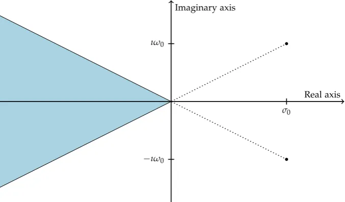
Willems et al. [29] provide a simple criterion on the poles of the closed loop system ˙

x= (A11+B1F1)xsuch that the system(7)is positively stabilized. Denote the eigenvalues of A11 by Eλ(A11) = σ0±ıω0, where ω0 6= 0. The closed loop system (7) with u =

max{0,F1x1}is stable ifF1is designed such that the eigenvaluesEλ(A11+B1F1) =σ±ωı

are taken inside the cone

σ+ıω∈C

σ<0 and

ω

σ <

ω0

σ0

, (8)

2. OVERVIEW OF LITERATURE

be mentioned that ifF1 is chosen such thatEλ(A11+B1F1) = {σ1,σ2}, possiblyσ1 =σ2,

thenualso yields an asymptotically stable system.

The criterion(8)can easily be visualised in the imaginary plane, as depicted inFigure 4. The blue shaded region highlites the region in which the poles of the system in controlled mode

˙

x(t) = (A+BF)x(t) may be placed to ensure stability. Ifω0 =0, then the eigenvalues

Eλ(A+BF)may be placed anywhere in the open left half plane.

Real axis Imaginary axis

σ0

ıω0

−ıω0

Figure 4: The blue shaded plane displays the allowable region in which the eigenvalues

E_λ(A+BF)may be placed.

The results of Willems et al.[29]can easily be supported by means of the following example.

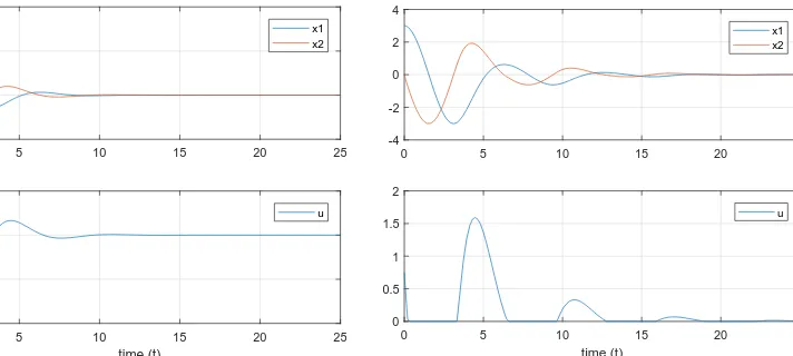
Example1. Consider for this example the system(2)with

A=

"

1 1

−1 1 #

and B= "

0 1 #

,

such that the rank ofC_{A,B}equals 2. The eigenvalues ofAare equal to 1±ı. According to (8), the system is stabilized by the positive control with eigenvaluesEλ(A+BF) =−1±12ı in controlled mode. This is indeed confirmed by the results of a simulation of this system which is included inFigure 5. On the other hand, Willems et al.[29]yields no guarantee thatEλ(A+BF) =−

1

2±ıresults in stabilization of the system. Figure 5shows the result of this simulation. It is obvious that the system is not asymptotically stable.

In a similar fashionFigure 4can be ‘reproduced’ by placing the eigenvaluesE_λ(A+BF) on some grid.Figure 7shows the result of a brute force series of simulations, where each simulation considers a poleplacement ofA+BFat someσ±ıω(so conjugate transpose pairs), with gridsσ =[-.1:-.1:-4.9]andω =[0:.1:4.9]. The case whereω =0 was extended with an additional pole on the real axis on the same grid as was used forσ. Figure 7plots theEλ(A+BF) =σ±ıωwhich resulted in a stabilized system green, and

thoseEλ(A+BF) =σ±ıωthat did not stabilize the system red. The figure shows a clear

resemblance with (the theoretic)Figure 4. 4

2. OVERVIEW OF LITERATURE

0 5 10 15 20 25

-40 -20 0 20 40

x1 x2

0 5 10 15 20 25

time (t) 0

20 40 60

u

Figure 5: Results of a simulation withEλ(A+BF) =−1±12ı(stable).

0 5 10 15 20 25 -4000

-2000 0 2000 4000

x1 x2

0 5 10 15 20 25

time (t)

0 2000 4000 6000 8000

u

Figure 6: Results of a simulation withEλ(A+BF) =−12±ı(not stable).

-5 -4 -3 -2 -1 0 1 2

Real axis

-5 -4 -3 -2 -1 0 1 2 3 4 5

Imaginary axis (i)

1+i

1-i outcome stable outcome not stable original pole

3.

T

he four

-

dimensional problem

The approach ofSection 2.2reduces the originaln-dimensional positive control problem(2) to a two dimensional problem. The problem is called ‘two-dimensional’ in the sense that the system hastwonon-stable poles, or in the sense that the feedback matrixF=hf1 f2

i

containstwodegrees of freedom to place thetwopoles of A+BF. This section continues with the problem described inSection 2.2, and extends it to a system for which matrixA

has at most two pairs of unstable complex conjugate eigenvalues, where the control input

u(t)is scalar. Thereby then-dimensional positive control problem can in a similar fashion be reduced to a four dimensional problem. The question that rises is if such a system can be stabilized with ascalarpositive state feedbacku(t).

With an extension to the four-dimensional problem, the problem is similarly extended to a six-dimensional, eight-dimensional or any higher ordereven-dimensional problem. Note that only the even dimensional problems are considered, and that for example the three dimensional problem is not considered. In case of any odd dimensional problem Ahas an odd number of eigenvalues. Hence at least one of the eigenvalues must be purely real, since only an even number can form complex conjugate pairs. If this real eigenvalue is negative, then it is not of interest for the positive control stabilization problem. If on the other hand this eigenvalue is positive, then there always exist initial conditions for which the system cannot be stabilized via positive control.

In terms of the illustrative pendulum problem fromSection 1.3the four-dimensional control problem with scalar input considers for example two pendula on which the exact same force u(t) is excerted. Intuitively one could excert a forceu on the pendula whenever

bothpendula move against the direction of force u, just as was done in the pendulum example. This could yield a state feedback matrix of the formF= [0,a1, 0,a2], for some scalara1,a2>0. Such an approach could work as long as there is a time span in which both pendula move against the direction of u. One can imagine a situation in which both pendula have the same eigenfrequency.4 Then there exist initial conditions such that there is never a time span in which the pendula move in the same direction, and hence there is never control input. This illustrates that the positive control problem with scalar state feedback may not be as trivial for the four dimensional problem as it is in the two dimensional problem. Hence, the criterion for stability as presented inWillems et al.may not be as simple for the four dimensional problem.

Formally, consider again the system(2), wherex(t) ∈Rn_{, A∈R}n×n _{andB ∈R}n×1_{. In} order for A to have (at most) two pairs of non-stable complex conjugate pole pairs, it should hold thatn≥4. For the case considered, letu(t)be a scalar positive state feedback of the formu(t) =max{0,Fx(t)}, withF∈R1×n_{. At this point, matrix Fneed not be fixed,}

but may for example be dependent onx, such that one could writeF(x). Such types of nonlinear control will be adressed later in this section.

The assumptions from Willems et al.[29]concerning the stabilizability of the pair(A,B) andEλ(A)∩R+ are maintained here. SinceWillems et al.already considered the cases

where Ahas zero or one stable (but not asymptotically) or unstable conjugate pole pair, these cases do not have to be reconsidered here. Only the case whereAhas exactly two unstable complex conjugate pole pairs are considered here.

Following the aproach of Willems et al.[29], consider system matricesAfor which there exists a nonsingular transformation T and a corresponding state vector ˜x = Txwhich

4_{It should be mentioned that if Ahas purely imaginary eigenvalues with same eigenfrequency, that is}

Eλ(A) ={±ωı,±ωı}, then the pair(A,B)is not controllable. For controllability to hold for systems with the

3. THE FOUR-DIMENSIONAL PROBLEM

separates the states into ˜x=hx1 x2 x3 it

, withx1,x2∈R2andx3∈Rn−4, such that(2) can be transformed into

˙

x1= A11x1+B1u, x1(0) =xa (9a)

˙

x2= A22x2+B2u, x2(0) =xb (9b)

˙

x3= A33x3+B3u, x3(0) =xc (9c)

with A11 and A22 anti-stable, A33 asymptotically stable (possibly of dimension 0), and (A11,B1),(A22,B2)stabilizable. Since A33is asymptotically stable, it holds that the state vectorx3∈L2for any inputu∈L2. Therefore the subsystem(9c)is not of so much interest for finding a stabilizing positive state feedback. The problem of stabilizing (9)can be reduced to finding a stabilizing input for both(9a)and(9b). In the case considered now,

u(t)is scalar and no two distinct controlsu1andu2can be excerted.

It should be mentioned that the notation of ˜xwill not used throughout this report. Instead the system is assumed to be of the form(9), with x=hx1 x2 x3

it .

3.1.

B

rainstorm on approaches

Willems et al. [29] provide conditions under which subsystems (9a) and (9b) can be positively stabilizedindividually. That is, it is known howF1andF2should be chosen for

u1=max{0,F1x1}andu2=max{0,F2x2}to be stabilizing positive feedback controls for (9a)and(9b)respectively.

It may be tempting to simply letF=hF1 F2 i

such that the control input is computed as

u=max{0,F1x1+F2x2}. This however yields no guarantees for the stability of the system. First of all since ifu>0 the subsystems are given by

˙

x1=A11x1+B1F1x1 + B1F2x2, ˙

x2=A22x2+B2F2x2 | {z }

as in[29]

+ B2F1x1 | {z } disturbances

,

where clearly the ‘first part’ is in line with Willems et al.[29], but the cross terms act as ‘disturbances’ between the systems. Furthermore, if(9a) requires controlu = F1x1 >0 and at the same time(9b)requiresu=F2x2>0 , then applying the control computed as

u=F1x1+F2x2is a too large input for either subsystem. One could argue to computeu as a weighted average of the two controls asu =max{0,aF1x1+ (1−a)F2x2}, for some

a∈(0, 1), in order to make a trade-off between the two systems. However, no guarantee for stability follows via Willems et al.[29]. Another rather important aspect is that Willems et al. [29]pose conditions on the eigenvalues ofA11+B1F1, which in that paper is equivalent to the eigenvalues of the system. Here, an additional system is present and one should be careful that in generalEλ(A+BF)6=Eλ(A11+B1F1)∪Eλ(A22+B2F2).

The suggested controls described above violate the original switching planes F1x1=0 and

F2x2=0. In any case, these planes indicate when their respective subsystem should receive some positive control input and when not, according to the result of Willems et al.[29]. This suggests a control law of the form

u(t)>0 if(F1x1(t)>0)∧(F2x2(t)>0)

u(t) =0 otherwise

It is debatable what the value of u(t) should be whenever positive. It may be de-sired that the control is at least proportional to x. One could for example take u(t) =

3. THE FOUR-DIMENSIONAL PROBLEM

max{F1x1(t),F2x2(t)}, or computeu(t)as some weighted average ofF1x1andF2x2 (when-ever positive). Note that the criterion(F1x1(t)>0)∧(F2x2(t)>0)may be very restrictive on the time span in which control is applied. Moreover, if the subsystems have the same eigenfrequency, i.e. ω1 = ω2, then there exist initial conditions such that the criterion (F1x1(t)>0)∧(F2x2(t)>0)is never satisfied.

Another variation such control could be

u(t) =     

    e

F1x1(t) +Fe2x2(t) if(F1x1>0)∧(F2x2>0)

F1x1(t) if(F1x1>0)∧(F2x2≤0)

F2x2(t) if(F1x1≤0)∧(F2x2>0)

0 otherwise,

for someFe₁andFe₂of appropriate size, possibly chosen asaF₁and(1−a)F₂respectively for somea∈(0, 1).

More of these types of control can be thought up, but none of these examples yield a guarantee for stability based on Willems et al.[29]only. In other words, the examples above illustrate that the separate results for F1 and F2 cannot simply be copied to the four-dimensional problem.

It may make more sense to look at the poles of the controlled system as a whole:Eλ(A+BF).

One of the conclusions from Willems et al.[29] is that pole placement on the real axis renders the positive control system stable, no matter the eigenvalues ofA11. Intuitively, in line with Willems et al.[29], one could presume that placing the poles ofEλ(A+BF)on

the negative real axis would suffice in stabilizing the system withu(t) =max{0,Fx(t)}= max{0,F1x1(t) +F2x2(t)}. This approach is considered in the following example.

Example2. Consider the system given byEquations (9a)and(9b)with

A11= "

0 1

−1 0 #

, A22= "

0 3

−3 0 #

and B=h0 1 0 1i t

.

The eigenvalues ofAare given byEλ(A) ={±ı,±3ı}, and hence are stable eigenvalues

(but not asymptotically). Therefore without control input the system’s states cannot explode. In this example the state feedbacku(t) =max{0,Fx(t)}is computed such that in controlled mode A+BF has its eigenvalues placed on the negative real axis. Two configurations are considered in this example, namelyEλ(A+BF) = {−2,−3,−4,−6},

andE_λ(A+BF) = {−3,−4,−6,−7}. Simulations were run with initial condition x0 = h

3 1 2 1i t

. Figures 8 and 9show the result for the former set of eigenvalues, and Figures 10and11for the latter set.

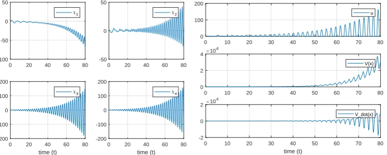
The results speak for themselves. If the poles for controlled mode are placed at Eλ(A+ BF) ={−2,−3,−4,−6}, then the simulation shows a stabilization of the states atx=0, whereas placement atEλ(A+BF) ={−3,−4,−6,−7}shows an unstable result. Note that

this example considers a stable (but not asymptotically) system. That is, the eigenvalues of

Aare purely imaginary, and hence the ‘exploding’ character that is presented inFigures 10

and11is solely due to the control inputu. 4

As the previous example shows, placing all poles of A+BF on the negative real axis does not guarantee an asymptotically stable system, in contrast to the result in Willems et al.[29]. There the result is based on the following observation: If the eigenvalues of

3. THE FOUR-DIMENSIONAL PROBLEM

0 10 20 30

0 1 2 3 4 1

0 10 20 30

-3 -2 -1 0 1 2

0 10 20 30

time (t) -2 0 2 4 3

0 10 20 30

time (t) -4 -2 0 2 4

Figure 8: State trajectories for eigenvalues

Eλ(A+BF) ={−2,−3,−4,−6}.

0 5 10 15 20 25 30

time (t) 0 1 2 3 4 5 6 7 8 9 10 u

Figure 9: Control input for eigenvalues

Eλ(A+BF) ={−2,−3,−4,−6}.

0 10 20 30

0 2 4 6 8 1

0 10 20 30

-5 0 5

2

0 10 20 30

time (t) -10 -5 0 5 10 3

0 10 20 30

time (t) -10 -5 0 5 10 4

Figure 10: State trajectories for eigenvalues

E_λ(A+BF) ={−3,−4,−6,−7}.

0 5 10 15 20 25 30

time (t) 0 10 20 30 40 50 60 u

Figure 11: Control input for eigenvalues

E_λ(A+BF) ={−3,−4,−6,−7}.

findsF1x(t) =F1e(A11+B1F1)(t−t0)x0, which can have at most one zero (since the eigenvalues of A11+B1F1 are real). This zero already occured at t = t0, and thus there will be no switch back to incontrolled mode. No such guarantee can be given for the four-dimensional system.

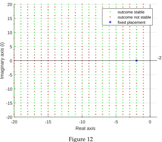
To further backup that the results from Willems et al.[29]cannot trivially be copied to the four-dimensional problem, considerFigure 12. A similar strategy asFigure 7was tried. As it is harder to visualize the four-dimensional problem in a two-dimensional plot, two of the placed poles were fixed at−2 for this example. The others were placed at a similar grid as inFigure 7. It should be mentioned that the system used to generate this plot is a different one than in the previous example.Figure 12was generated using a matrix Afor whichE_λ(A) ={±ı,±2ı},B=h1 0 1 0i

t

andx0= h

1 1 1 1i t

. The figure is just included as an indication that a clear bound on the poleplacement is not as clearly marked out as in the two-dimensional problem.

3. THE FOUR-DIMENSIONAL PROBLEM

-20 -15 -10 -5 0

Real axis

-20 -15 -10 -5 0 5 10 15 20

Imaginary axis (i)

-2 outcome stable outcome not stable fixed placement

Figure 12

3.2.

M

otivation

The examples in the previous section show that the four-dimensional problem should be approached in a different way. It is clear that the results from the two-dimensional problem as described by Willems et al.[29]provide no direct guarantee for a stabilizing positive control for the four-dimensional problem. The goal of the remainder of this report is to investigate control laws for stabilizing the four-dimensional problem, as to form an extension to the problem considered in Willems et al.[29]. Hence, in contrast to some of the suggested control laws of the previous section, the positive state feedback control law of the form

u(t) =max{0,Fx(t)},

will be considered, where the state feedback matrixFis invariant of time and state. The following section wraps up this chapter by stating a formal problem statement. This formally describes the problem that is considered throughout this report.

Section 5and Section 4individually propose two separate techniques to approach the four-dimensional positive control problem with the above described control law. Section 4 proposes a control law based upon Lyapunov’s stability theory. Thereafter,Section 5applies techniques of singular perturbations for ordinary differential equations to the positive control problem. Approaching the problem via singular perturbations allows the re-use of the approach considered in Willems et al.[29].

3.3.

F

ormal problem statement

Consider only the four-dimensional non-stable subsystem extracted from(9)given by

" ˙

x1 ˙

x2 #

= "

A11 0

0 A22 # "

x1

x2 #

+ "

B1

B2 #

3. THE FOUR-DIMENSIONAL PROBLEM

Denote the eigenvalues of AbyEλ(A) ={σ1±ω1ı,σ2±ω2ı}such that

Eλ(A11) =σ1±ω1ı and Eλ(A22) =σ2±ω2ı. (10b)

Note thatσ1,σ2≥0 andω1,ω2∈R. Let the positive control state feedback be given by

u(t) =max{0,F1x1(t) +F2x2(t)}. (10c)

The question is whether such positive state feedback (10c)can be designed such that it stabilizes the system(10a)with eigenvalues(10b).

Based on the sign ofF1x1+F2x2the system(10a)switches between the uncontrolled mode (11a)and the controlled mode(11b)below

" ˙ x1 ˙ x2 # = "

A11 0

0 A22 # " x1 x2 # , (11a) " ˙ x1 ˙ x2 # = "

A11+B1F1 B1F2

B2F1 A22+B2F2 # " x1 x2 # = "

(A11+B1F1)x1+B1F2x2 (A22+B2F2)x2+B2F1x1 #

. (11b)

where(11a)holds whenF1x1+F2x2≤0, and(11b)holds whenF1x1+F2x2>0.

Some words should be dedicated to the notation that is used. In general, capital letters are used to indicate (sub)matrices, and lower case letters for their entries. For matricesA,B

andFthis indicates the following general notation:

A=

"

A11 0

0 A22 # =     

a11 a12 0 0

a21 a22 0 0

0 0 a33 a34 0 0 a43 a44 

   

, B= " B1 B2 # =      b1 b2 b3 b4      ,

F=hF1 F2 i

=hf1 f2 f3 f4 i

.

The reader should be aware that for example for A22this yields the somewhat unfortunate notation of

A22= "

a33 a34

a43 a44 #

.

The state vector is always written as lower case, its subvectors are also written as lower case. This poses possible ambiguity for the notation of the state vectorxelementwise. As a solution, theith element ofxis denoted byχ_{i, such that}

x= " x1 x2 # =      χ₁ χ₂ χ₃ χ₄      .

Just as forA22, be aware that in this notationx2= h

χ₃ χ₄

it .

4.

L

yapunov approach

Lyapunov proposed two methods for demonstrating stability. Lyapunov’s second method, which is referred to as theLyapunov’s stability criterion, uses aLyapunov function, commonly denoted byV(x). A Lyapunov function is a scalar function defined on the state space, which can be used to prove the stability of an equilibrium point. The Lyapunov function method is applied to study the stability of various differential equations and systems.

This section uses theory of Lyapunov to design a stabilizing positive control law for stable systems inSection 4.2. The application of such control law for unstable systems is considered inSection 4.3. The following section covers some of the necessary background on Lyapunov stability theory.

4.1.

L

yapunov stability theory

Consider then-dimensional system of differential equations

˙

x(t) = f(x(t)), x(t0) =x0∈Rn, t≥t0, (12)

with equilibrium x=0. Suppose we have a functionV:Rn _{→Rthat does not increase}

along any solutionx(t)of(12), i.e., that

V(x(t+τ))≤V(x(t)), ∀τ>0,

for every solutionx(t)of(12). Now ifV(x(t))is differentiable with respect to timetthen it is nonincreasing if and only if its derivative with respect to time is non-positive everywhere, so

˙

V(x(t))≤0 ∀t.

Using the chain-rule one finds

˙

V(x(t)) = dV(x(t))

dt =

∂V(x(t)) ∂x1

˙

x1(t) +· · ·+

∂V(x(t)) ∂xn x˙n

(t)

= ∂V(x(t)) ∂x1

f1(x(t)) +· · ·+

∂V(x(t))

∂xn fn

(x(t)) =: ∂V(x) ∂xt f(x)

_x=x(t), (13)

where

∂V(x) ∂xt =

h

∂V(x)

∂x1

∂V(x)

∂x2 . . .

∂V(x)

∂xn i

.

In order to derive stability from the existence of a non-increasing functionV(x(t)) it is additionally required that the function has a minimum at the equilibrium. It is furthermore assumed thatV(x¯) =0. The main theorem follows.

Theorem 4(Lyapunov’s second stability theorem (as for instance presented in[17])) Con-sider(12)with equilibriumx. If there is a neighbourhood¯ Ωofx and a function V¯ :Ω→Rsuch that onΩ

1. V(x)is continuously differentiable,

2. V(x)has a unique minimum onΩinx,¯

3. ∂V(x)

∂xt f(x)≤0for all x,

then x is a stable equilibrium, and then V¯ (x) is called a Lyapunov function. If in addition

∂V(x)

4. LYAPUNOV APPROACH

An additional condition called ‘radial unboundedness’ is required in order to conclude global stability. The functionV(x)isradially unboundedifV(x)→∞as||x|| →∞. Then the theorem on global asymptotic stability reads as follows:

Theorem 5 If V:Rn→Ris a strong Lyapunov function forx on the entire state space¯ Rnand V(x)is radially unbounded, then the system is globally asymptotically stable.

For Lyapunov stability of linear state space models, consider the linear system(10). With state feedback control, i.e. u=Fx, the system can be rewritten as

˙

x= (A+BF)x=Axe . (14)

For these types of systems the following theorem holds.

Theorem 6(Lyapunov equation (as presented in[17])) Let A∈Rn×n_{and consider the system}

˙

x(t) =Ax(t)with equilibrium pointx¯=0∈Rn_{. Suppose Q∈R}n×n_{is positive definite and let}

V(x0):= Z ∞

0 x t

(t)Qx(t)dt (15)

in which x(0) =x0. The following three statements are equivalent.

1. x¯=0is a globally asymptotically stable equilibrium ofx˙(t) =Ax(t).

2. V(x)defined in(15)exists for every x∈Rn _{and it is a strong Lyapunov function for this}

system. In fact, V(x)is then quadratic, V(x) = xt

Px, with P∈ Rn×n_{, the well defined}

positive definite matrix

P:=

Z ∞

0 e At

t_QeAt_{dt. (16)}

3. The linear matrix equation

At

P+PA=−Q (17)

has a unique solution P, and this P is positive definite. The quadratic function V(x) =xt

Px is aLyapunov functionfor this system.

In that case the P in(16)and(17)are the same.

If inEquation (17)Pis positive definite andQis positivesemi-definite (seeDefinition B.1b), then all trajectories of ˙x(t) = Ax(t)are bounded. This means that all eigenvalues of A

have nonpositive real part. Equation (17)is called thecontinuous Lyapunov equation. The existence of a solution of which is covered in the following theorem:

Theorem 7(Continuous Lyapunov equation) Let A,P,Q∈ Rn×n _{where P and Q are}

sym-metric. Given any Q which is positive definite, there exists a unique positive definite P such that

At

P+PA=−Q (18)

if and only if all eigenvalues of A have negative real part.

Consider the candidate Lyapunov functionV(x) = 1₂xt

Pxfor the positive control system (10a). Recall that in this case a four dimensional problem is concerned, so n = 4. Let

P ∈ R4×4 _{be a symmetric positive definite matrix of the form P =} "

P1 0

0 P2 #

, with

P1,P2 ∈ R2×2 also positive definite, such that the candidate Lyapunov function can be rewritten as

V(x) = 1₂xt

1P1x1+12x t

2P2x2. (19)

4. LYAPUNOV APPROACH

For sure, thisV(x)satisfies the first two conditions ofTheorem 4sincePis positive definite, andV(x)is quadratic inxhence positive definite relative to ¯x=0. Note also thatV(x)is radially unbounded. Recall that a positive control system is considered. Therefore, it is desired thatV(x)is a Lyapunov function for the system ˙x= Ax+Bu, for allu>0 as well as foru=0. For the derivative ofV(x(t))with respect to time, denoted by ˙V(x(t)), one finds

2 ˙V(x) =x˙t

1P1x1+xt1P1x˙1+x˙t2P2x2+xt2P2x˙2

= (A11x1+B1u)tP1x1+xt1P1(A11x1+B1u) + (A22x2+B2u)tP2x2+xt2P2(A22x2+B2u) = (xt

1A t 11+B

t

1u)P1x1+xt1P1(A11x1+B1u) + (x2tA t 22+B

t

2u)P2x2+xt2P2(A22x2+B2u) =xt

1(A t

11P1+P1A11)x1+xt2(A t

22P2+P2A22)x2+ (xt1P1B1+B1tP1x1+B2tP2x2+xt2P2B2)u =xt

1(A t

11P1+P1A11)x1+x t 2(A

t

22P2+P2A22)x2

| {z }

=:V_P(x)

+2(xt

1P1B1+x t 2P2B2)u

| {z }

=:V_u,P(x)

, (20)

where the time variabletis ommitted for notational purposes. Expression(20)is obtained sinceBt

iPixi = (BtiPixi)t=xtiP t

iBi = xtiPiBi,i=1, 2, by the symmetry ofPi(i.e. Pit= Pi)

and by any scalar being equal to its transpose.

4.2.

C

ontrol design for stable systems

ForV(x)to be a Lyapunov function, the third condition inTheorem 4requires that ˙V(x)≤0 for allx and for all non-negative control valuesu. A closer inspection ofEquation (20) reveils that one way ˙V(x)≤0 may be achieved is via the following conditions:

1. The positive definite matricesP1andP2are chosen such that(A₁₁t P1+P1A11)and (At

22P2+P2A22)are either negative (semi-)definite, or equal to the zero matrix. If such matricesPican be found then thexti(A

t

iiPi+PiAii)xiterms,i=1, 2, are quadratic in

xi and for sureVP(x)≤0∀x.

2. The control law foruis designed such thatVu,P(x)≤0∀x.

If both conditions hold, then obviously ˙V(x)≤0 for allx. The existence of suchP1and

P2is linked toTheorem 7. It states that for systems ˙x =Ax+Buwith Aasymptotically stable, there exists positive definite matricesP1andP2such that A11t P1+P1A11 ≤0 and

At

22P2+P2A22≤0. For the case where all eigenvalues ofAare purely imaginary, as will be shown later, there do exist positive definite matricesP1andP2such that A11t P1+P1A11=0 andAt

22P2+P2A22=0. This section considers systems for which the set of eigenvalues of

Ais equal to

Eλ(A) ={±ω1ı,±ω2ı}, ω1,ω2∈R>0 (21)

where±ω1ıare the eigenvalues ofA11 and±ω2ıare the eigenvalues ofA22. That way A may be assumed to be of the form

A=

"

A11 0

0 A22 #

, where A11 = "

0 ω1 −ω1 0

#

and A22= "

0 ω2 −ω2 0

# .

Note that one findsAt

ii=−Aii,i=1, 2. In this case there exist positive definite matricesP1 andP2such that

At

11P1+P1A11 =0, (22a)

At

4. LYAPUNOV APPROACH

Conditions(22)hold for any matricesP1andP2which are positive multiplications of the identity matrix. Formally conditions(22)are satisfied for

P1=c1I, P2=c2I, (23)

wherec1,c2>0 andIdenotes the 2×2 identity matrix. This wayEquation (20)simplifies to

˙

V(x) = (xt

1P1B1+xt2P2B2)u= (Bt1P1x1+Bt2P2x2)u= (BtPx)u, (24)

where the second equality holds since(xt

1P1B1+xt2P2B2)is scalar, and therefore it equals its transpose.

Be aware thatBt

Pxmay be alternatingly positive and negative. For ˙V(x)≤0 to hold for allx, the control inputuis based upon the switching planeBt

Px=0 as follows:

u=0 if Bt

Px≥0,

u>0 if Bt

Px<0.

This wayV(x) as defined inEquation (19)is a Lyapunov function for the system Equa-tion (10a)with inputu, it is not a strong Lyapunov function though. A control law that suffices for stability isu = max{0,−Bt

Px}, which if written out yields the control law specified as

u(t) =max{0,−Bt

Px(t)}=max{0,−(Bt

1P1x1(t) +B2tP2x2(t))}. (25)

The positive control input(25)is of the state feedback formu=max{0,F1x1+F2x2}, with

F1=−B1tP1andF2=−Bt2P2. The question is whether this control yields anasymptotically

stable system.

Note that the control law designed in such way has two degrees of freedomc1,c2>0 for the matricesP1=c1IandP2=c2I. These parameters could be used to tune the controller, or determine the relative weight the controller puts on state setsx1andx2.

4.2.1. Motivation and simulations

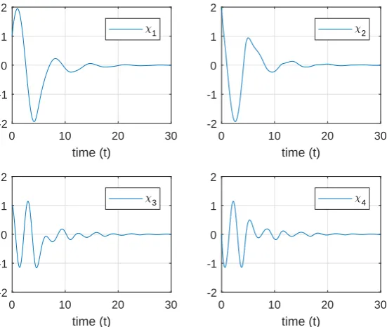
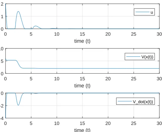
This section briefly shows the result of a simulation in which the Lyapunov based control law(25)is applied. By the design of this control law, it is expected that it asymptotically stabilizes systems for which the eigenvalues of the state matrixAare purely imaginary. This expectation is supported by means ofExample 3. In this example the control law(25) is applied in a simulation of a ‘parallel pendulum system’.

Example3. Consider the system(10a)withω1=1 andω2=2, such that

A11 = "

0 1

−1 0 #

and A22 = "

0 2

−2 0 #

.

Furthermore letB1 = B2= h

0 −1i t

, and inEquation (25)letP1= P2 = I2×2. For this

simulation let the initial state vector be equal tox0= h

1 2 1 0i t

. In terms of pendula, this example considers two pendula with different eigenfrequencies (due to different length/weight ratios), and different initial conditions. The results of the simulation are shown inFigures 13and14.

The simulation shows a couple of aspects. First of all, for this example the system is stabilized at ¯x=0 by a control inpututhat is non-negative. Furthermore,Figure 14shows that indeed ˙V(x)≤0 for all time andV(x)is nonincreasing. All these observations live up to the expectations of the behaviour of the system.

4. LYAPUNOV APPROACH

0 10 20 30

time (t)

-2 -1 0 1 2

1

0 10 20 30

time (t)

-2 -1 0 1 2

2

0 10 20 30

time (t)

-2 -1 0 1 2

3

0 10 20 30

time (t)

-2 -1 0 1 2

4

Figure 13: Simulation results for state trajectoriesx.

0 5 10 15 20 25 30

time (t)

0 1 2

u

0 5 10 15 20 25 30

time (t)

0 5 10

V(x(t))

0 5 10 15 20 25 30

time (t)

-4 -2 0

V_dot(x(t))

Figure 14: Simulation results for control inputuand Lyapunov functionV(x)and its time derivative ˙V(x).

Also for a complete illustration, the plots of a simulation of the system withω1=ω2=2 is included.Figures 15and16show the typical result ofV(x)being non-increasing, but converging to a constant value instead of converging to 0, that is, statexconverges to some

trajectory inRn. 4

4. LYAPUNOV APPROACH

0 10 20 30

time (t)

-4 -2 0 2 4

1

0 10 20 30

time (t)

-4 -2 0 2 4

2

0 10 20 30

time (t)

-4 -2 0 2 4

3

0 10 20 30

time (t)

-4 -2 0 2 4

4

Figure 15: Simulation results for state trajectoriesx.

0 5 10 15 20 25 30

time (t)

0 1 2

u

0 5 10 15 20 25 30

time (t)

0 5 10

V(x(t))

0 5 10 15 20 25 30

time (t)

-4 -2 0

V_dot(x(t))

Figure 16: Simulation results for control inputuand Lyapunov functionV(x)and its time derivative ˙V(x).

4.2.2. Asymptotic stability

In order to analyze the stability of the positive control system(10a) with control (25), it makes sense to first investigate the behaviour ofBt

Px(t) which is used in(25). Can it be the case that given some initial timet0 and state x(t0) = x0 with BtPx0 > 0 that

Bt

Px(t)remains positive for allt≥t0? In that caseu(t)remains 0 for allt≥t0 and the system remains ‘stuck’ in uncontrolled mode. The following theorem states under which conditionsBt

Px(t)is ensured to change sign from positive to negative, which is needed to reach controlled mode.