Context trees : augmenting geospatial trajectories with context

warwick.ac.uk/lib-publications

Original citation:

Thomason, Alasdair, Griffiths, Nathan and Sanchez Silva, Victor. (2016) Context trees :

augmenting geospatial trajectories with context. ACM Transactions on Information Systems,

35 (2). 14.

Permanent WRAP URL:

http://wrap.warwick.ac.uk/79709

Copyright and reuse:

The Warwick Research Archive Portal (WRAP) makes this work by researchers of the

University of Warwick available open access under the following conditions. Copyright ©

and all moral rights to the version of the paper presented here belong to the individual

author(s) and/or other copyright owners. To the extent reasonable and practicable the

material made available in WRAP has been checked for eligibility before being made

available.

Copies of full items can be used for personal research or study, educational, or not-for profit

purposes without prior permission or charge. Provided that the authors, title and full

bibliographic details are credited, a hyperlink and/or URL is given for the original metadata

page and the content is not changed in any way.

Publisher’s statement:

"© ACM, 2016. This is the author's version of the work. It is posted here by permission of

ACM for your personal use. Not for redistribution. The definitive version was published in

ACM Transactions on Information Systems, 35(2) 2016

http://doi.acm.org/10.1145/2978578

A note on versions:

The version presented here may differ from the published version or, version of record, if

you wish to cite this item you are advised to consult the publisher’s version. Please see the

‘permanent WRAP url’ above for details on accessing the published version and note that

access may require a subscription.

Context Trees: Augmenting Geospatial Trajectories with Context

Alasdair Thomason, Nathan Griffiths, Victor Sanchez

Department of Computer Science,

University of Warwick, UK

June 2016

Abstract

Exposing latent knowledge in geospatial trajectories has the potential to provide a better under-standing of the movements of individuals and groups. Motivated by such a desire, this work presents thecontext tree, a new hierarchical data structure that summarises the context behind user actions in a single model. We propose a method for context tree construction that augments geospatial trajectories with land usage data to identify such contexts. Through evaluation of the construction method and analysis of the properties of generated context trees, we demonstrate the foundation for understanding and modelling behaviour afforded. Summarising user contexts into a single data structure gives easy access to information that would otherwise remain latent, providing the basis for better understanding and predicting the actions and behaviours of individuals and groups. Finally, we also present a method for pruning context trees, for use in applications where it is desirable to reduce the size of the tree while retaining useful information.

1

Introduction

Exposing the latent knowledge present in geospatial trajectories has become an increasingly important research topic in recent years, due in part to the pervasiveness of location-aware hardware and the resulting availability of trajectory data. Motivated by a desire to understand the movement patterns of users, this paper presents a new data structure, thecontext tree, that summarises the context behind user actions in a single hierarchical model. Additionally, the paper proposes a method for generating context trees from geospatial trajectories and land usage information, and provides concrete implementations for each stage of the method, namely augmentation, filtering, and clustering. A context tree itself is formed of clusters at multiple scales that describe the contexts in which the user was immersed, affording easy access to information that would have previously remained hidden, forming the basis for understanding and predicting the actions and behaviours of individuals and groups.

Existing work in understanding people through the context of activities has considered various at-tributes as defining context, including an individual’s location, the current time and weather, and other individuals who are nearby [Dey and Abowd, 1999; Schilit et al., 1994], typically using data collected from smartphones [Bao et al., 2011; Cao et al., 2010; Huai et al., 2014]. While existing approaches provide a basis for context-aware applications, they are limited by the data that can be collected directly from the user. Augmenting geospatial trajectories with land usage information enables the identification of contexts that consider the type and properties of the location of an activity.

In this paper we present the following contributions: (i) the context tree data structure that hier-archically represents user contexts at multiple scales, (ii) a method for constructing context trees from geospatial trajectories and land usage information, (iii) a set of concrete techniques to achieve each stage in the construction method, namely augmentation, filtering and clustering, (iv) evaluation of context trees constructed from real-world data, and an analysis of the properties that make them amenable for

use in understanding individuals, and (v) a method of pruning context trees, to reduce their size while retaining useful information.

The remainder of this paper is structured as follows. Section 2 discusses relevant related work in location extraction and activity and context identification. In Section 3 we propose the context tree, a new data structure, and present an overview of the method employed for constructing context trees. Concrete implementations of the stages of this method are given in Sections 4 and 5. We present an evaluation of context trees in Section 6, and discuss pruning the generated trees in Section 7. Finally, we conclude the paper with a discussion of future work and applications in Section 8.

2

Related Work

Geospatial trajectories, usually collected from GPS logging devices, have been used as a basis for knowl-edge acquisition in many areas, including for location extraction [Andrienko et al., 2011; Ashbrook and Starner, 2002, 2003; Bamis and Savvides, 2011; Montoliu and Gatica-Perez, 2010; Thomason et al., 2015a, 2016]. Periods of low mobility are extracted from the trajectories and clustered using techniques such as DBSCAN [Ester et al., 1996] and k-means [MacQueen, 1967], identifying areas in which the time was spent. These techniques identify areas of arbitrary shape, but are incapable of identifying places where non-stationary activities took place. Augmenting identified areas with additional information, Yan et al. [2013] propose a technique for the derivation and modelling ofsemantic trajectories. However, the additional data sources are not leveraged for identifying locations, only for providing labelling after locations have been identified.

Once identified, significant locations have formed the basis for many applications, including location prediction using Markov models [Ashbrook and Starner, 2002, 2003], neural networks [Thomason et al., 2015c], periodicity-based approaches [Wang and Prabhala, 2012], and blockmodels [Fukano et al., 2013]. Using multilayer perceptrons for location prediction, Thomason et al. [2015b] evaluate extracted loca-tions and predicloca-tions to perform automatic parameter selection for location extraction and prediction. Research has also considered predicting when a user will next visit a specific location using Bayesian inference [Gao et al., 2012], how long a user will stay at a given location [Liu et al., 2013], as well as developing techniques to apply labels in a semi-supervised manner to extracted locations to provide addi-tional meaning [Krumm and Rouhana, 2013]. Prediction has also occurred without the need for location extraction, in the form of destination prediction, achieved by identifying similar historical trajectories to a current one through clustering approaches [Chen et al., 2010; Monreale et al., 2009; Nakahara and Mu-rakami, 2012], Bayesian inference [Krumm and Horvitz, 2006] and hidden Markov models [Alvarez-Garcia et al., 2010]. Similarly, predicting journey duration has been explored using neural networks [Chen et al., 2009], along with predicting when two people will next meet [Yu et al., 2015], and providing recommen-dations to users new to a city based on the locations visited by others [Bao et al., 2015; Zheng and Xie, 2010].

While trajectories have also been used to identify non-stationary activities, in the form of transport mode identification through change-point detection and classification-based approaches [Liao et al., 2007; Patterson et al., 2003; Zheng et al., 2008a,b], many related techniques operate on different sources of data. Activity detection has been achieved from video data by Kim et al. [2010], who use Markov models to identify the activities being performed. Unfortunately, ensuring the constant availability of video data on an individual is infeasible. Research has therefore considered identifying the activity being performed from low-level sensor data (e.g. accelerometers and heart-rate) generated by devices carried by individuals, using classifiers and related techniques to label periods of data from a set of possible activities [Choudhury et al., 2008; Lee and Mase, 2002; Lester et al., 2005; Morris and Trivedi, 2011; Pirttikangas et al., 2006; Ravi et al., 2005].

et al., 2015], with specific examples in defence [Howard, 2002] and aviation [Endsley, 1995, 2000]. As with location extraction, however, existing techniques focus only on collected data, and do not attempt to augment this with other data available after collection. Such augmentation could offer greater insight into the entities a person was interacting with, enabling a better understanding of the actions they were performing.

Focusing on only trajectories, literature has also considered the identification of repeating patterns, both from geospatial trajectories [Cao et al., 2005, 2007; Eagle and Pentland, 2009; Giannotti et al., 2007; Gudmundsson et al., 2004], and general object movement trajectories [Li et al., 2010; Yang et al., 2003], where repeating patterns are expected to consist of activities that the user repeatedly conducts. Such patterns have also been considered as routines, where the aim is to extract features of a given day for classification (e.g. “left work at 5PM”) [Farrahi and Gatica-Perez, 2008, 2010]. Patterns, and extracted location transitions, have formed the basis of user similarity identification [Xiao et al., 2012], and travel companion identification [Tang et al., 2012]. Once expected patterns for a given user or group have been extracted, anomalous actions become possible to identify. Anomaly detection has been performed on geospatial trajectories, where isolation-based outlier detection has identified anomalous subtrajectories from vehicle tracking data [Chen et al., 2011; Zhang et al., 2011]. Similarly, statistical approaches have been shown to be useful in identifying trajectories that differ from an expected pattern [Laxhammar and Falkman, 2011, 2014; Rosen and Medvedev, 2012].

Raw geospatial trajectories have been used as the basis for many different tasks and applications. While assuming the availability of additional data at time of collection is often infeasible, augmenting trajectories after collection is possible and can enrich the knowledge afforded. Applications that consider such augmented trajectories include using map data to fill in missing periods of a trajectory [Zheng et al., 2012], and using map searches augmented with trajectories from the same user to enhance destination prediction [Wu et al., 2015]. While existing work by Yan et al. [2013] has considered the augmentation of trajectories to understand the semantics behind trajectory segments, they do not attempt to utilise the semantics to influence the partitioning of trajectories or identify contexts. Understanding the semantics behind trajectories from the beginning has the potential to better understand what a person was doing and their interactions, and thus provide a foundation for identifying similar contexts.

2.1

Geospatial Datasets

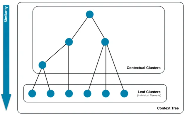
Figure 1: An abstract representation of a context tree, in which the similarity of nodes increases with depth.

2.2

Investigative Techniques

For many techniques relating to extracting knowledge from data, collecting a concrete ground truth is infeasible. Significant location extraction, for example, can extract locations at various scales and so no single ground truth can exist. Existing literature addresses this by exploring the properties of the outputs from such techniques and comparing these properties to expected results. For instance, Guidotti et al. [2015] create synthetic trajectories with known properties and devise metrics to compare extracted locations with desirable properties. Thomason et al. [2015a] compare properties of the identified locations against acceptable ranges of values, determined from knowledge of the input data, as well as demonstrating the applicability of the technique through examples. For travel-mode classification, Si la-Nowicka et al. [2015] compare against a small set of manually labelled subtrajectories. In this paper, to cope with the limited availability of user-provided ground truth, we present an evaluation that both compares the output of the proposed approach to a limited ground truth and characterises the outputs of the algorithm through a set of metrics. While a ground truth may not exist in all domains, an understanding of the performance and applicability of the proposed approach can be achieved through characterising the outputs and manually generating or labelling subsets of the data to create a partial ground truth.

3

Proposed Structure: The Context Tree

This paper proposes and evaluates the context tree hierarchical data structure, that summarises the contexts that a user has been immersed within at multiple scales. Each leaf node of the tree represents a real-world feature or element that the user has likely interacted with, be it a specific building, area, or individual feature (e.g. a bench in a park). These individual elements are joined together through

context nodes that represent a context at a specific scale, where time spent within a context means that the user likely had similar aims or goals, and are identified by exploring time the user spends interacting with elements with similar properties, or elements that are interacted with in a similar manner. As it summarises time in this way, the context tree can become the basis for understanding people from augmented geospatial data. The context tree structure is depicted in Figure 1.

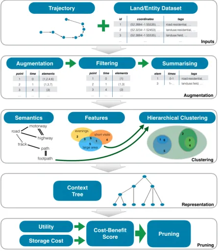
1. Inputs

The raw geospatial trajectory and land usage data enters the system.

2. Augmentation

Land usage elements likely to have been interacted with are identified by extracting all potential elements and filtering them to remove noise.

3. Clustering

Filtered land usage elements, and their interactions, become the basis for contextual clustering. Clustering is achieved with a hierarchical agglomerative algorithm.

4. Representation

Once clustered, the elements form a context tree data structure that can be used as the basis for further understanding the behaviours of individuals and groups.

5. Pruning

Some applications may be limited by the amount of data they can store, or processing they can perform, and so it may be necessary to prune a context tree to reduce its size while maintaining as much useful information as possible. Pruning is achieved through analysing the nodes of a context tree with respect to a defined set of metrics.

In the following sections we describe the stages of augmentation (Section 4), clustering (Section 5), representation (Section 5), and pruning (Section 7) in more detail.

4

Trajectory Augmentation

In order to better understand users through their past actions, and assuming only geospatial data is available at the point of data collection, this section describes the process of trajectory augmentation that combines raw trajectories with land usage data. A trajectory is a temporally ordered sequence of data points that locate an individual or entity:

T = (p1, p2, p3, ..., pn)

where pi = {ti, li, ai} is an individual trajectory point, consisting of time (ti), location (li, e.g. a < lat, lng >pair) and accuracy (ai, typically measured in metres).

In addition to such trajectories, land usage data can also be used for identifying locations and entities that are meaningful to the user. Land usage data is assumed to be sets of entities with associated information. An entity, in this case, directly maps to a single real-world object, feature, or area, such as an individual postbox, field, or building. It can also refer to a collection of such entities that form a larger designation, such as a university campus or residential housing area. Each of these elements is expected to be associated with a set of geographical coordinate pairs that represent its shape and location, in addition to a set of tags in the form of ‘key:value’ pairs that describe properties of the element, including its type and usage (e.g. a house may be tagged as ‘building:residential’).

4.1

Element Extraction

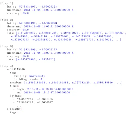
The process for extracting relevant land usage elements is illustrated in Figure 3. A raw geospatial trajectory (Step 1) is overlaid on a land usage dataset (Step 2), at which point the accuracy recorded by the location measuring device (e.g. GPS, measured in metres) is used (Step 3), such that all elements that are partially or wholly within the radius are stored alongside the original trajectory point (Step 4). This procedure is completed automatically by iterating through each trajectory point and querying the land usage dataset for any element that intersects or covers any part of the accuracy radius.

4.2

Filtering

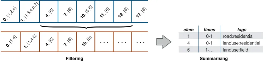
Figure 3: Trajectory augmentation procedure.

Figure 4: Example of filtering augmented trajectories to remove noise, and subsequent summarising through clustering of contiguous time periods.

procedure can be used. Our proposed filter is a generalised version of a weighted average filter, a technique typically used to smooth noisy signals, modified to operate over sets of land usage elements and depicted in Figure 4. The filter maintains a buffer of elements and selects from this buffer based on an assigned weight in a three-step process:

1. A buffer of points, and associated land usage data, is selected.

2. The land usage elements in the buffer are weighted and scored.

3. Elements are selected, based on their score, for inclusion in the output.

4.2.1 Buffer Selection

ALGORITHM 1 Buffer Management

1: points ←(p1, p2, ...)//input set

2: δ←300//input parameter specifying buffer width

3: buffer ←[points.shift ]

4: output ←[ ]

5: index ←null

6:

7: //Build the initial buffer

8: whilepoints.length>0do

9: //Ifindex has not been set, then we are in the first half

10: if index == null && TimeBetween(buffer[0],points[0])> δthen

11: //If the next point is greater thanδseconds from the first, then the first half is full

12: index ←buffer.length−1

13: //Ifindex has been set, then we are in the second half

14: else if index ! = null && TimeBetween(buffer[index],points[0])> δthen 15: break//Exit the loop as adding the next point would exceedδ

16: else

17: buffer.append(points.shift)

18: end if

19: end while

20:

21: //Process the current buffer, incrementindexand maintain the new buffer

22: whilepoints.length>0do

23: output.append(Filter(buffer,index))//Perform the actual filtering 24: index ←index + 1

25:

26: //If the point for consideration is not in the buffer, then add it now

27: if index ==buffer.lengththen

28: buffer.append(points.shift)

29: end if

30:

31: //Remove any point from the first part that is not withinδseconds ofbuffer[index]

32: whileTimeBetween(buffer[0],buffer[index])> δdo

33: buffer.shift

34: index ←index - 1

35: end while

36:

37: //Add points until doing so would exceedδseconds from buffer[index]

38: whilepoints.length>0 && TimeBetween(buffer[index],points[0])<=δdo

39: buffer.append(points.shift)

40: end while

41: end while

42:

43: returnoutput

4.2.2 Scoring

Scores are then applied to each land usage element in the buffer, weighted by the number of points the element is associated with, the accuracy of these points and the temporal distance from the point under consideration. Since we are dealing with sets, rather than the filter simply averaging values over the buffer, the process is modified by assigning weighted scores to each set element and then selecting elements according to a threshold. Combining these factors into a score, we have:

Score(e) = X p∈Pe

₁

ap

×

1−dist(p, pc)

δ

× |Pe| (1)

dist(p1, p2) is the number of seconds between pointsp1 andp2(temporal distance). Equation 1 gives a

higher score to elements associated with a large number of high accuracy points (where high accuracy is recorded as a small value). Scores are then normalised relative to the maximum:

N ormalisedScore(e) = Score(e)

argmaxScore(Score(e) :∀e∈buffer)

(2)

4.2.3 Selection

With each element in the buffer assigned a score, selection can occur either by using a fixed threshold to discard low-scoring elements, or by keeping all elements but limiting their effect through soft-thresholding. Soft-thresholding is a technique commonly applied in signal processing, where a kernel is applied to the calculated scores, forcing higher scores closer to 1 and lower scores closer to 0. While soft-thresholding removes the need to apply a fixed threshold, for this work we are only concerned with whether or not an element is included in the output set and thus we employ a threshold, t, where any element with a N ormalisedScoreof greater than t becomes part of the output set, and the remaining elements are discarded.

4.3

Data Summarisation

Once filtered, augmented trajectories contain a record of where an individual was at a given time, along with the real-world features they were likely interacting with. These interactions are summarised into continuous spans of time by considering each land usage element encountered. If the same land usage entity is associated with two consecutive points, it can be assumed that it is also associated with the period of time between these points, if such a period of time is sufficiently small. An example summary is shown in Figure 4 (right).

If the time between consecutive points is large, it cannot be known whether the user ceased interacting with an element and resumed again before data collection next occurred, and so a limit on the time between consecutive points is specified as tmax. If the time between two consecutive points associated with the same element is greater than tmax, then the interactions are split, a technique also used in location extraction applications [Montoliu and Gatica-Perez, 2010; Thomason et al., 2016]. This results in a summary list of land usage elements along with a set of times, during which the individual can be assumed to have been interacting with the element in question.

5

Contextual Clustering

The identification of similarcontexts is performed through clustering that considers both the properties of the elements and the properties of user interactions to determine similarity. Rather than aiming to identify a single level of clusters, which would limit the utility and applicability of the clusters to a single scale, the goal here is to build a hierarchical model, constructed by progressively merging land usage elements that represent similar contexts in a context tree, a depiction of which is shown earlier in Figure 1.

5.1

Building Clusters

Initially, each land usage element is distinct and is treated as a singleton cluster (i.e. a cluster with exactly one element). At each round of clustering, several of these clusters are merged to represent a context and a new higher level in the hierarchy, with pointers between the levels considered as parent

andchild relationships. That is, if two clusters at one level become merged into another cluster at the next level, the original clusters are considered aschildren of the new cluster. This section describes how clusters are merged with respect to their properties.

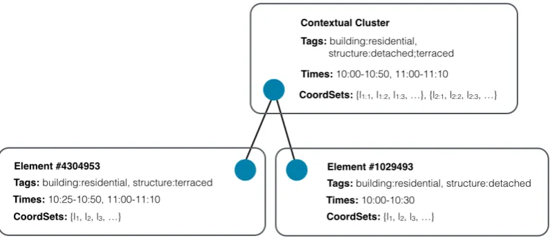
Figure 5: Cluster merging example.

Times

The times for the merged cluster are taken to be the union of the sets of times from all child clusters, where overlapping time ranges are themselves combined into one. For example, if one cluster had the set of times{10:00-10:05, 11:00-12:00} and another had{10:04-10:20, 11:10-11:15, 12:05-12:09}, then the merged times would be{10:00-10:20, 11:00-12:00, 12:05-12:09}.

Tags

Similarly, each element has associated tags. The tags of the merged cluster are defined as the union of tags from the child clusters, where if two tags share a key but not a value, both values are stored.

Geographical Coordinate Sets

Each element contains a set of coordinates that define the geographical shape of the entity to which they relate. Merging such elements should keep each of these sets discrete, unless they intersect, in which case the coordinates belonging to both shapes are combined and replaced with their convex hull.

The merging of Times assumes a periodicity of 24 hours, which while reasonable for many people (i.e. those who follow a daily routine), it may not be appropriate for everyone. As such, automatic time series learning could be utilised to better learn meaningful movement patterns of the individual. While exploring such techniques is beyond the scope of this paper, there are many existing approaches that may be effective for the task [Ahmad et al., 2004]. An example merging of two elements according to these rules is shown in Figure 5, where it is assumed that there is no geographical overlap between the two elements (i.e. the coordinate sets cannot be merged).

5.2

Contextual Distance Metrics

Clustering elements together requires a distance metric to measure element similarity. While identifying contexts from certain types of data is a task considered before, and discussed in Section 2, no metrics currently exist that have been tailored to the identification of contexts from augmented geospatial tra-jectories. This section presents metrics that encapsulate the goals behind context extraction for this specific problem, with an emphasis on properties of the interactions and properties of the real-world features being interacted with. Having defined how elements are merged into clusters and, consequently, how two clusters are merged (Section 5.1), we can now consider the similarity between two clusters.

5.2.1 Semantic Similarity

with similar tags are likely to have properties in common, we use the semantic similarity between cluster tags as the basis for a distance metric. For this, we adopt the similarity measure proposed by Wu and Palmer [1994], and extended by Resnik [1999] for calculating distance between word taxonomies through WordNet [Miller, 1995]. The calculated scores are between 0 and 1 (inclusive), where a score of 1 means that the words are interchangeable. The semantic similarity between two sets of tags, t1 and t2, is

therefore calculated as:

T agSim(t1, t2) =

P

t∈t1argmaxSim(Sim(t, t21), Sim(t, t22), ..., Sim(t, t2i))

|t1|

(3)

As tag similarity is not commutative, cluster similarity is calculated as:

SemanticSimilarity(c1, c2) =

argmaxT agSim(T agSim(c1.tags, c2.tags), T agSim(c2.tags, c1.tags)) (4)

5.2.2 Feature Similarity

The context of an activity or period of time is dependent not only on the location in which time is spent, but on additional factors. With this in mind, we propose a second similarity measure,FeatureSimilarity, that compares the interaction features of two clusters, specifically:

• Average interaction duration

• Most common time of day interaction begins

• Count of the number of times the element is interacted with

• Total area covered by elements (inm2₎

The value from each feature is then discretised by placing values within bins (e.g. time of day could be recorded in 4 hour increments), and converted into a single string that describes the feature and value (e.g. ‘timeofday 12’ would indicate that the most common time of day that interaction begins is between 12PM–4PM). This procedure generates a set of features,f1andf2, for clustersc1andc2, from which a

similarity score is defined using the Jaccard index [Rajaraman and Ullman, 2011]:

F eatureSimilarity(f1, f2) =

|f1∩f2| |f1∪f2|

(5)

5.2.3 Geographical Distance

For some applications it is possible that the similarity between clusters depends upon their geographical proximity, where two clusters that are close together may have common purposes. If this property is known to be true in the data, or given the goal of clustering, then the proximity of clusters can be considered as the minimum geographical distance between elements of a cluster, calculated using the Haversine formula [Robusto, 1957]:

GeographicalDistance(c1, c2) =argmindistance(distance(x1∈c1, y1∈c2), . . .) (6)

5.2.4 Hybrid Contextual Distance

Using one of the previously discussed metrics in isolation would not accurately capture the context of the individual, as context depends on more than just any one factor. Instead, we combine the

SemanticSimilarity andFeatureSimilarity scores intoHybrid Contextual Distance (HCD), a measure of the contextual similarity between two clusters:

HCD(c1, c2) =

1−(λ×SemanticSimilarity(c1, c2) + (1−λ)×F eatureSimilarity(c1, c2)) (7)

ALGORITHM 2 Agglomerative Hierarchical Clustering Algorithm

1: clusters ←elements//The input set ofelements, each treated as its own cluster

2: whileclusters.length>1do

3:

4: //Create ann×nmatrix of distances between clusters

5: distanceMatrix ←[ [d11, ...],[d21, ...], ...]

6:

7: //Find all pairs of clusters with the smallest distance between them

8: //If multiple pairs overlap (i.e. share a cluster), then group them together

9: closestGroups ←ClosestGroups(distanceMatrix)

10:

11: //Merge each extracted group into a single cluster

12: forgroup ∈closestGroups do

13: newCluster←Merge(group)

14:

15: //Set the old clusters as children of the new and remove the old clusters fromclusters

16: forcluster ∈group do

17: newCluster.children.append(cluster)

18: clusters.delete(cluster)

19: end for

20:

21: //Add the merged cluster toclusters

22: clusters.append(newCluster)

23: end for

24:

25: end while

26:

27: //By this point,clusters contains a single root cluster for the hierarchy

28: returnclusters.first

because contexts should be separate from their geographical location (e.g. visiting two cafes in different cities is likely to be indicative of the same context). If, however, additional domain knowledge is available that ties geographical locations together with additional meaning (e.g. it is known that all buildings in a given area perform a similar function), then geographical distance could be added to the HCD metric. HCD can be used as a basis for clustering elements, and thus determining which elements have similar contexts, aiding in our understanding of the individual to which the data belongs.

5.3

Hierarchical Clustering

With a distance metric in place, clustering can be performed using standard techniques. While tradi-tional clustering is limited in that it extracts clusters at a single scale, which may not be appropriate for a given task, hierarchical clustering identifies clusters at multiple scales. We use a greedy hierarchical agglomerative clustering algorithm, presented in Algorithm 2, that extracts clusters of increasing simi-larity up to a single root node, creating a context tree. While the hierarchical agglomerative clustering algorithm is fairly standard in itself, its application to the generation of context trees is novel. The algo-rithm deviates slightly from existing hierarchical clustering approaches in that it is capable of extracting multiple clusters together in a single step if they have the same distance.

6

Evaluation and Results

( S t e p 1 )

l a t l n g: 5 2 . 3 8 3 4 4 9 9 , −1.56026223

timestamp: 2013−11−08 14:09:5 1 . 0 0 0 0 0 0 0 0 0 Z

a c c u r a c y: 6 5 . 0

( S t e p 2 )

l a t l n g: 5 2 . 3 8 3 4 4 9 9 , −1.56026223

timestamp: 2013−11−08 14:09:5 1 . 0 0 0 0 0 0 0 0 0 Z

a c c u r a c y: 6 5 . 0

d a t a: [ n 3 1 2 8 7 3 2 9 5 , n 5 5 2 1 0 1 2 0 8 , n 6 9 5 9 4 2 9 2 6 , n 1 0 1 4 5 8 5 8 4 5 , n 1 0 1 4 5 8 5 8 5 3 , w 92341980 , w 92342116 , w 145179860 , w 145179863 , w 145179883 ,

w 273005393 , w 303748830 , w 329376738 , w 329376739 , r 2 4 3 7 0 2 3 , . . . ]

( S t e p 3 )

l a t l n g: 5 2 . 3 8 3 4 4 9 9 , −1.56026223

timestamp: 2013−11−08 14:09:5 1 . 0 0 0 0 0 0 0 0 0 Z

a c c u r a c y: 6 5 . 0

d a t a: [ w 145179860 , r 2 4 3 7 0 2 3 ]

( S t e p 4 )

w 145179860:

t a g s:

b u i l d i n g: u n i v e r s i t y

b u i l d i n g l e v e l s: 3

members: [ n 1 5 8 6 1 8 5 8 6 3 , n 1 5 8 6 1 8 5 8 8 3 , n 7 2 7 3 8 2 4 2 5 , n 1 5 8 6 1 8 5 8 5 6 , . . . ]

t i m e s:

- b e g i n: 2013−11−08 13:13:0 5 . 0 0 0 0 0 0 0 0 0

end: 2013−11−08 17:16:4 7 . 0 0 0 0 0 0 0 0 0

l a t l n g s:

- 5 2 . 3 8 3 7 7 6 5 , −1.5601465 - 5 2 . 3 8 3 8 2 8 5 , −1.5600527 - . . .

r 2 4 3 7 0 2 3:

t a g s: . . .

Figure 6: Examples of the data at each stage of the augmentation and filtering processes.

utility afforded by these procedures.

This section evaluates the proposed context tree data structure, along with the generation method proposed in Sections 4 and 5. Although there are many use-cases for context trees, including as a basis for anomaly detection, location prediction and city planning, we focus on understanding the high-level behaviours of an individual throughout a 24 hour period as a representative example.

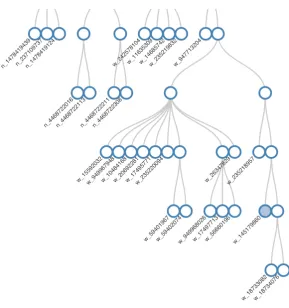
Figure 7: An extract of a tree generated using real data. The element used in the previous data examples is located in the bottom right of the image, clustered with other university buildings.

6.1

Data

Evaluating this work requires both geospatial trajectories and land usage information. The trajectories used are taken from the Nokia Mobile Data Challenge (MDC) Dataset [Kiukkonen et al., 2010; Laurila et al., 2012], as discussed in Section 2.1. From this dataset, we select the real-world data from 40 users with the largest number of trajectory points for this evaluation. While this dataset contains a vast amount of information, we only consider the timestamp, latitude, longitude and accuracy of each data point (consistent with the discussion in Section 4). In addition to this, and for comparative purposes, we also select 5 users from the GeoLife dataset [Zheng et al., 2008a, 2009, 2010] for evaluation. While the MDC dataset aims to provide continuous coordinates for the users, the GeoLife data instead only captures periods of times when the users were moving. It has the additional drawback of not including accuracy values, which are required for this work. As the data was collected using GPS-enabled devices, we opt to assume a constant accuracy of 10m for each coordinate, in line with the expected performance of GPS [Cao et al., 2009]. The trends presented in this section are consistent across both the MDC and GeoLife data, and so most of the GeoLife results are omitted for brevity, however an example can be found in Section 6.5.

A major drawback of using research datasets is that licences often prevent the publication of details that can be used to identify people or specific locations visited. Additionally, it is not possible to contact the users about whom data was collected to perform a user study. To get around these issues, we also collect a small dataset of our own. Aiming to match the methodology of the MDC data, trajectories were collected from the smartphones of 3 members of the Department of Computer Science, University of Warwick for a period of 3 days. These trajectories are used for illustration, instead of the MDC data, in Section 6.4 where the presented results contain the names of specific locations visited, and communication with the users was required.

Land usage information comes from OpenStreetMap (OSM)1_{, a community-maintained map that}

0 20 40 60 80 100

0.0 0.1 0.2 0.3 0.4 0.5 0.6 0.7 0.8 0.9 1.0

%

Element Weighting

Figure 8: Distribution of element weights before filtering for an example user (δ= 1200).

0 500 1000 1500 2000 2500

0 0.2 0.4 0.6 0.8 1

Av erag e Elemen ts p er P oin t t

(a)t(δ= 1200)

0 20 40 60 80 100 120

0 1000 2000 3000 4000

Av erage Elemen ts p er P oin t δ

(b)δ(t= 0.8)

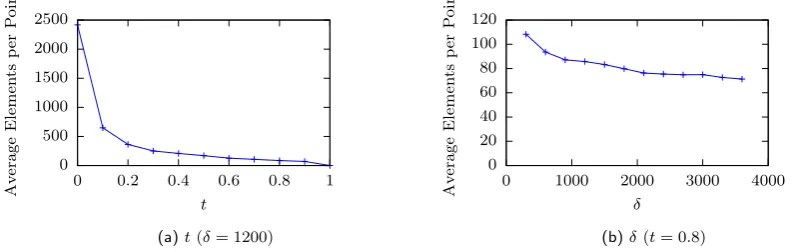
Figure 9: Effect of parameters on average number of elements per point post-filtering for an example user.

contains information pertaining to real-world entities, including their geographical coordinates and a set of tags that describe the entity. These entities include features such as individual items (e.g. a payphone or postbox), through to buildings and general land-usage designations (e.g. ‘farmland’). The data is extremely detailed and accurate, spanning the entire world in a consistent manner, and thus forms an ideal basis for this work. The required elements are extracted from OSM through the Overpass API2.

6.2

Filtering

The first stage in context tree generation is augmenting and filtering land usage elements. This section evaluates and characterises the performance of the filter on real-world data, by first exploring how element weights are distributed and then showing how this impacts the land usage elements that are filtered.

Filtering takes two parameters: δandt. The parameterδspecifies the width of the buffer, in seconds, andtspecifies a threshold where elements with a calculated weight of greater thantform the output set. Holdingδ= 1200, Figure 8 shows the distribution of weights for all elements in the filtering process (i.e. the values ofNormalisedScore from Equation 2) for all 11,575 trajectory points belonging to a sample MDC user. The effects of t (with δ = 1200) and δ (with t = 0.8) on the average number of elements per point post-filtering can be seen in Figures 9a and 9b, respectively. These results are consistent with expectations, as increasingt sets a higher threshold for elements to be included in the output set, and thus results in fewer elements. Increasing δ results in a greater time span considered by the filtering process, and so more elements are considered as transient, and are thus removed. Each of these figures is generated from 7 months of data from a single sample user, and while the exact numbers vary when using data from different users, the trends remain consistent across users from both datasets.

The accuracy of the trajectory points determines the radius of land usage data to consider. The effect of accuracy on the number of extracted elements, both pre- and post-filtering, is shown in Figure 10 for each of the 40 MDC users. The figure demonstrates that a larger accuracy typically results in a larger number of elements per point, and that filtering reduces this number.

2_{https://wiki.openstreetmap.org/wiki/Overpass_API— By default, the Overpass API is only capable of extracting}

16 32 64 128 256 512 1024

70 75 80 85 90 95 100 105 110 115

Av

erage

Elemen

ts

p

er

P

oin

t

Accuracy (m) Raw

Filtered

Figure 10:Effect of accuracy on number of elements, pre- and post-filtering, for different users’ data.

0 0.02 0.04 0.06 0.008.1 0.12 0.14 0.16 0.018.2

0 200 400 600 800 1000

Av

erage

Key

Similarit

y

Trajectory Point Raw

Filtered

Figure 11: Effect of filtering on tag key similarity, both pre- and post-filtering.

6.2.1 Filtering Characterisation

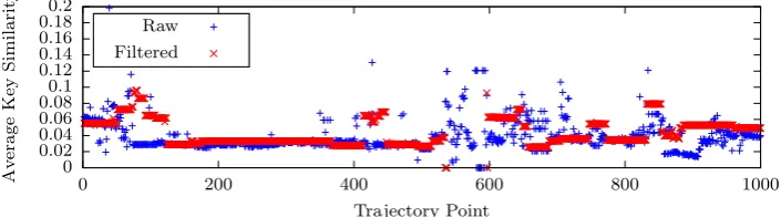
To better understand the filtering process, we explore properties of the filtered data, specifically focusing on how the elements and their semantics change. The aim of filtering is to remove noise and focus the data on elements that the user was likely interacting with at a given time. It is reasonable therefore to assume that the elements post-filtering should have more similarity than those before, with less variation caused by the inclusion of random elements. To explore this hypothesis, Figure 11 shows the average tag key similarity (i.e. only the key part of the ‘key:value’ pair that makes up an element’s tags, which corresponds to broad type, e.g. ‘building’) both pre- and post-filtering for a given user over 1000 points of their data. This demonstrates that in the majority of cases, tag key similarity is increased, and variance significantly reduced, after filtering has occurred, indicating that the elements present post-filtering are more similar and that unrelated noise elements have been correctly removed. The semantic similarity of these tags is calculated using the method proposed in Section 5.2.1.

6.3

Summarising Data

Once the data has been filtered, it is summarised into continuous periods of time. Only one parameter,

tmax, is required, specifying the maximum amount of time (in seconds) between consecutive points for

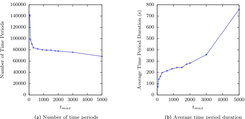
them to be considered contiguous. Using the parametersδ= 1200 and t = 0.8, Figure 12a shows how tmax affects the number of such periods extracted, and Figure 12b shows how tmax affects the average length of such periods.

0 20000 40000 60000 80000 100000 120000 140000 160000

0 1000 2000 3000 4000 5000

Num b er of Time P erio ds tmax

(a)Number of time periods

0 100 200 300 400 500 600 700 800

0 1000 2000 3000 4000 5000

Av e rage Time P erio d Duration (s) tmax

(b)Average time period duration

Figure 12: Effect oftmaxon the summarising procedure.

6.4

User-informed Evaluation

While there is no ground truth available for this type of problem, we can evaluate the procedure by considering desirable properties of the output for a specific application and manually compare the ex-pected and actual results for small subsets of data. A major problem here is that when conducting such evaluations over publicly available research datasets, such as the MDC or GeoLife datasets used in this paper, or alternatives such as Yonsei, there is no mechanism for contacting users to have them verify assumptions. To overcome this problem, we opt to use data collected ourselves for this part of the evaluation, as it affords us the ability to discuss with users exactly what activities they were conducting on a given day. Details of the data collected can be found in Section 6.1.

This section presents analyses on small amounts of manually labelled real-world data with the goal of using the constructed context trees to provide meaning to high-level behaviours, with the overall aim of identifying such behaviours from the tree. The data analysed spans 24 hours from the three users of the Warwick dataset, where annotations were added manually as accurately as possible, and in consultation with the users. The augmentation and filtering procedures were run over this data and, for each labelled time period, the 3 most common element tags were identified. This is shown in Figures 13-15. The aim here is not to label the time periods with the exact activity being performed, but rather to demonstrate that a meaningful relationship exists between the tags extracted and the true activity.

In Figure 13, general labels are applied to the activities being performed, and a meaningful correlation between the tags extracted by the procedure and these labels is evident. Specific examples include the action of driving being labelled with the ‘highway’ key, and taking the train with ‘railway’. Although the tags are not always perfect, they are indicative. For instance, when the individual was at home no residential building was identified, but an indication of the type of location was given by the tags ‘lit:yes’ and ‘highway’. In the region where this data was collected, roads with street lighting typically signify residential areas. A similar relationship is shown in Figures 14 and 15, with labels applied hierarchically and at lower granularities. While not every item is labelled exactly, we believe this is a result of the data collection method. We used a data collection rate of one point per minute, meaning that several labelled activities consist of only 1 or 2 trajectory points, leaving little information for the procedure to utilise. Similarly, the land usage dataset contains a vast amount of information, but can be limited in parts. An example of this is that the pub which was visited at 17:25 (Figure 14) is inside a larger building. The procedure is only capable of identifying that the building was occupied by the user, but there is no information pertaining to which element inside the building was being interacted with, and so the only available information is ‘building:yes’.

Figure 13: Manually labelled data (in bold) compared against extracted element labels.

well correlated to the activity (e.g. ‘building:residential’ to the activity ‘Home’),medium indicates that there is some link (e.g. ‘surface:asphalt’ to ‘Driving on a main road’), andlow/none being given to tags with little or no relationship to the activity (e.g. ‘highway:bus stop’ to ‘Attending lecture’). Figure 16a shows the proportion of tags assigned to each of these weightings, demonstrating that the procedure identified tags with high or medium relevancy 69.7% of the time. We also consider the highest-ranked tag assigned to each labelled time period and the proportion of time periods represented by each tag score is shown in Figure 16b. From these results, it is clear that while in the three examples, only 32.8% of tags were awarded ahighrelevancy score, 60.0% of labels have at least one tag with such a score, and 88.9% contain at least one tag with a score ofhigh ormedium. This indicates that while not all of the 3 tags per label were useful, in nearly all cases, at least one of them was.

Table 1: Summary of tags and frequency count for each type of interactions scored based on the relevancy of each tag (High, Medium and Low/None).

Label Tag S # Tag S #

Home landuse:residential H 2 barrier:kissing gate L 1

highway:residential H 2 oneway:no L 1

building:residential H 1 maxspeed:30 L 1

building:garage M 1 highway:primary L 1

lit:yes M 1 left county:nor... L 1

Walking (res.) landuse:residential H 1

Walking (shops) amenity:parking M 1

Walking (road) sidewalk:both H 2 highway:bus stop M 1

highway:secondary H 1 bicycle:yes M 1

oneway:yes M 2 ref:lmngtns L 1

lit:yes M 2 public transport:pay... L 1

boundary:public... L 1

Walking (park) leisure:park H 1 waterway:river M 1

foot:yes H 1 barrier:gate M 1

barrier:kissing gate M 1

Driving (res.) landuse:residential H 2

Driving (road) highway:tertiary H 6 maxspeed:60 M 3

highway:primary H 2 maxspeed:30 M 2

highway:secondary H 1 maxspeed:20 M 2

oneway:yes M 4 amenity:university L 2

highway:bus stop M 3 type:multipolygon L 1

surface:asphalt M 3

Parking (uni) amenity:university M 1 type:multipolygon L 1

Work (office) building:university H 2 highway:footway L 1

building levels:4 M 2 highway:service L 1

Walking (uni) amenity:university H 4 landuse:grass M 1

highway:crossing H 2 type:multipolygon L 4

Eating (rest.) level:0 M 1 area:yes L 1

level:1 M 1 lit:yes L 1

building:yes M 1 surface:asphalt L 1

Eating (pub) building:yes M 1 area:yes L 1

level:0 M 1

Work (library) amenity:library H 2 type:multipolygon L 2

amenity:university M 2

Work (lecture) surface:asphalt L 2 highway:bus stop L 1

type:multipolygon L 1 oneway:yes L 1

lit:yes L 1

Visiting friend amenity:university M 1 type:multipolygon L 1

building:yes M 1

Petrol station operator:tesco H 1 amenity:fuel H 1

opening hours:24/7 H 1

Union (uni) amenity:university M 1 type:multipolygon L 1

Bar building:yes M 2 oneway:yes L 2

surface:asphalt L 2

Train electrified:rail H 2 railway:rail H 1

Figure 15: Manually labelled data (in bold) compared against extracted element labels.

40 (32.8%)

45 (36.9%)

37 (30.3%)

(a)Overall tag relevancy

High Medium Low/None

No Tags 27 (60.0%)

13 (28.9%) 4 (8.9%)

1 (2.2%)

(b)Best tag relevancy per time period

0 50 100 150 200 250 300

0 0.2 0.4 0.6 0.8 1

T

ree

No

des

λ(Semantic Weighting)

Total Avg. Children per Node

Figure 17:Relationship betweenλand number of tree nodes.

Figure 18: Example context tree: geographic clustering.

6.5

Context Trees

When constructing context trees from summarised data (Section 5), the only required parameter is λ, which specifies the weighting to be given tosemantic similarity as part of theHybrid Contextual Distance

distance metric (Equation 7). A weighting of 1 will construct a tree based only on the semantic similarity between node tags, and a weighting of 0 will construct a tree based only on the similarity of features, with any value in between using a combination of the two. The relationship betweenλand the number of nodes in a context tree is shown in Figure 17 (generated using 24 hours of a single users’ data, filtered with parameters δ = 1200, t = 0.8, and tmax = 1200). While the number of nodes does not vary drastically withλ, the meaning behind the clusters does.

Figure 19:Example context tree: temporal clustering.

Figure 20: Example context tree: semantic clustering (λ= 1).

distance between elements (Figure 18) and temporal distance between interactions (Figure 19). While these figures only show one small example, the results are representative of using such metrics in that the elements clustered together have no clear contextual relationship. This is in contrast to the context trees generated from the same data using the Hybrid Contextual Distance metric, along with different values ofλ, as shown in Figures 20–22.

In all of these examples, the element identifier has been manually replaced with a descriptive key-word to represent the element. Semantic clustering (Figure 20) creates distinctive groups for buildings, footpaths and public amenities, as the elements in these groups are similar, while feature-based cluster-ing (Figure 21) creates groups that are less easily identifiable and relate to properties of the elements (e.g. the footpaths are not grouped because they were not encountered in the same journey, but rather were used at different times of the day). Finally, hybrid clustering (Figure 22) shows properties of both semantic and feature-based clustering where both the description of the element and properties of the interaction with the element are considered to create clusters. Selecting an appropriate value of λ is application-specific.

Figure 21:Example context tree: feature-based clustering (λ= 0).

providing an indicator of the utility of this approach in lieu of a ground truth. The assumptions made are:

1. Buildings should be grouped together unless they have very different uses (e.g. residential buildings should not be in the same group as office buildings).

2. Roads should be grouped together, with elements relating to roads grouped at a higher level (e.g. junctions).

3. Public amenities should be grouped together unless the interactions have very different properties.

These assumptions focus on the semantics of elements, but the features also need to be considered when exploring possible reasons for clusters being split. For instance, if a person visited many houses as part of their job, it would be reasonable to assume that these houses should be semantically close to the residence of the individual in the context tree, but not at exactly the same level. The usefulness of such assumptions will depend on the application, but it is possible to see that when aiming to characterise how a person has spent their time, it is beneficial to identify the times spent at residential buildings separately to those spent at work. On the small example context trees shown in this section, geographic and temporal clustering (Figures 18 and 19) violate all 3 assumptions. Semantic clustering (Figure 20) best adheres to these assumptions, with the houses grouped at the same level and the building under construction close by in the next level up. Similarly, the footpaths are together with the cycle barrier, a related element, and highway one level up. Feature-based clustering (Figure 21) has fewer valid assumptions than semantic clustering, as it only considers the interactions with the elements and not the elements themselves. Although the houses are together in a single cluster, they are also joined with the car park and footpath. Finally, hybrid clustering (Figure 22) is very similar to semantic clustering with the exception that the highway is no longer situated close to the footpaths, but is further up the context tree by itself. This still leaves 2 of the assumptions strictly adhered to, with 1 very close. A change that can be explained by the consideration of interaction features, where the highway has a different profile of interaction than the footpath and cycle barrier elements. Again, these are small examples, however the trends present have been observed to be consistent across larger context trees.

Figure 22:Example context tree: hybrid clustering (λ= 0.6).

(where daynshows a summary for a tree built using all data from days 0 ton) are shown in Figure 24a. Please note that no data was recorded during day 5 for this sample user in the MDC dataset.

Figure 23 begins with a low coverage for bothFixed andRetrained lines, indicating that few elements encountered in day 1 were present in the training set (day 0). However, while theFixed score remains low for days 2–4, theRetrained score approaches 100%. In this instance, this is indicative of the user visiting elements that they did not encounter in the initial training day (day 0), but that they did encounter during subsequent days, as the Retrained line includes all previous days as training data. The figure shows similar results for the remaining test days, where during day 9 the user visited only locations visited during day 0 and during days 9, 11 and 16–20 the user encountered no new elements as the score forRetrained is at 100%. Figure 24a shows how these properties relate to the size of context trees generated. The number ofleaf nodes is the number of unique elements and the number oftime periods

is a count of the total number of (non-unique) elements encountered. That is, if the user encountered the same element 3 times, or 3 different elements, both would count as 3 time periods. At day 1 the number of time periods is roughly the same as the number of leaf nodes, indicating that all elements were encountered approximately once. As time goes by, more elements are encountered, but a large number of existing elements are revisited, demonstrated by the disproportionate rise in the number of time periods. This indicates that over a short period, where the user likely remained within a single region, the size of the tree does not increase significantly as additional data is added. However, considering trees over larger time periods will not have the same property as the user will likely visit new regions with entirely new leaf nodes. Figure 24b shows a similar graph as Figure 24a, however it was generated using data from a user of the GeoLife dataset instead of the MDC dataset. As is evidenced by the figures, the procedure extracts similar trends in users from each dataset.

0 20 40 60 80 100

0 5 10 15 20

Co

v

erage

(%)

Day

Fixed Retrained

Figure 23:Land usage coverage with an initial training period of 24 hours (indicated by the dotted line).

0 500 1000 1500 2000 2500 3000 3500 4000 4500 5000

0 5 10 15 20

Coun

t

Training Data (Days) Total Nodes

Leaf Nodes Time Periods

(a)MDC user

0 500 1000 1500 2000 2500

0 5 10 15 20

Coun

t

Training Data (Days) Total Nodes

Leaf Nodes Time Periods

(b)GeoLife user

Figure 24: Training data against number of tree nodes.

7

Context Tree Pruning

Storing context trees in their entirety maintains the maximum amount of information, however there are applications where reducing the size of a tree may be desirable. Memory-constrained devices, for example, may be better able to make use of a reduced size context tree as this would require lower storage requirements, and also enable quicker search due to the reduced number of nodes. Furthermore, reducing the size of context trees may have application-specific benefits, such as preventing overfitting when learning prediction models. In both of these cases, it is desirable to prune the tree to reduce the amount of data stored while maintaining as much information as possible. This section presents a method for such pruning, that although requires additional processing to select nodes eligible to be removed, results in smaller context trees that require less memory to store and fewer operations to search. A representation of a pruned context tree can be seen in Figure 25.

7.1

Pruning Criteria

Figure 25:An example of a pruned context tree (with removed nodes crossed through).

hypothesis, and the hypothesis rejected when the utility of storing the cluster is above a threshold. Any cluster for which we are unable to reject the hypothesis is pruned, and its parent is marked as eligible for pruning. As metrics do not already exist for this task, we adapt existing metrics used in related domains for the purpose of context tree pruning.

7.1.1 Storage Cost

Clusters are scored according to two metrics: their storage cost and their utility. To determine the cost of storing a cluster, it is important to understand how clusters are built up in a context tree (described in Section 5.1). When merging two clusters together to form a parent cluster, the aspects that belong to each cluster are considered in turn; specifically the tags, times andcoordinate sets. Sets of tags are combined from the child clusters by taking their union, while times and coordinate sets are merged in such a way that overlapping components are combined into single elements, and thus through the combining of child clusters into a parent cluster, information has been removed. The cost of storing an additional node is therefore the cost of storing the individual components (e.g. time range) that are present in a child, but not present in the same form in its parent. Assuming uniform cost for each component:

Cost(C|P) =

ξ+|Ctimes\Ptimes|+|Ccoordsets\Pcoordsets|+| ∪s∈Ccoordsetss\ ∪s∈Pcoordsetss| (8)

Whereξ >0 is a small, manually selected, penalty that represents the overhead of storing each cluster,

Ctimesis the set of time ranges that are associated with clusterC andCcoordsetsis the set of coordinate

sets associated with clusterC. Remembering that the coordinate sets belonging to a cluster themselves contain sets of points (i.e.Ccoordsets={{p1:1, p1:2, p1:3, ...},{p2:1, p2:2, p2:3, ...}, ...}),∪s∈Ccoordsetssis taken

to be the set of all points associated with any coordinate set that belongs to cluster C. Having ξ as non-zero represents that there is always a (small) cost associated with each cluster. Equation 8 will need tuning based on the specific application to better represent the true cost of storing a node, but it provides a basic foundation.

7.1.2 Cluster Utility

0 50 100 150 200 250 300

0 0.2 0.4 0.6 0.8 1

Num b er of Unpruned No des

Prune Thresholdθ

Node Count

(a)Node Count

0 0.2 0.4 0.6 0.8 1

0 0.2 0.4 0.6 0.8 1

HCD

Prune Thresholdθ

Average HCD

(b)Average HCD

0 5 10 15 20

0 0.2 0.4 0.6 0.8 1

Information

(

×

10

7)

Prune Thresholdθ

Information

(c)Total Information

Figure 26: Effect ofθon number of nodes in a sample context tree (λ= 0.5, ξ= 1).

(i.e. tags, times, and coordinate sets) present in each cluster:

Information(C) =P

t∈Ctimesduration(t) + P

s∈Ccoordsetsarea(s) +|Ctags| (9)

Providing even weighting to the different elements for the measure of utility:

Utility(C|P) = 1− 1

3

P

t∈Ctimesduration(t) P

t∈Ptimesduration(t)

+1 3

P

s∈Ccoordsetsarea(s) P

s∈Pcoordsetsarea(s)

+1 3

|Ctags|

|Ptags|

!

(10)

Specifically, this metric considers the proportion of time, area and tags covered by the child with respect to the parent, and holds true to the aims of such a metric to produce a score of 0 if the parent and child contain identical information and a score approaching 1 if the child only represents a fraction of the parent.

7.1.3 Cost-Benefit Score

Thecost-benefit score of a cluster is taken to be the utility of the cluster divided by the storage cost:

CostBenefitScore(C|P) = Utility(C|P)

Cost(C|P) (11)

While utility is normalised between 0 and 1 as it represents the proportion of the parent that is not covered by the child, cost only has a minimum bound of ξ (Section 7.1.1), where ξ > 0. Depending upon the application, it may be desirable to also normalise cost relative to the current context tree. Using this metric on nodes depth-first, pruning should occur for any cluster C with parent P and

CostBenefitScore(C|P)< θ, whereθis thepruning threshold andC has no unpruned children.

7.2

Pruning Evaluation

Pruning requires a pre-built context tree and two parameters, namely θ and ξ, where θ provides a threshold for pruning, andξ is a penalty associated with every node when calculating itsstorage cost.

0 20 40 60 80 100 120 140 160 180 200

0 0.5 1 1.5 2 2.5 3 3.5 4 4.5 5

Num b er of Unpruned No des ξ Node Count

(a)Node Count

0 0.2 0.4 0.6 0.8 1

0 0.5 1 1.5 2 2.5 3 3.5 4 4.5 5

HCD

ξ

Average HCD

(b)Average HCD

0 5 10 15 20

0 0.5 1 1.5 2 2.5 3 3.5 4 4.5 5

Information ( × 10 7) ξ Information

(c)Total Information

Figure 27:Effect ofξon number of nodes in a sample context tree (λ= 0.5, theta= 0.2).

the nodes present in the unpruned tree, but maintains almost 70% of the useful information. While the process to prune the context tree adds in additional complexity, the resultant tree is considerably more compact and thus applications that require storing or searching the tree will have significantly lower overhead.

Using the same data again, but this time holding θ= 0.2, Figure 27 shows the effect of changing ξ on the number of unpruned nodes, average HCD and information. Increasing eitherθ or ξ reduces the number of nodes left after pruning (Figures 26a and 27a), as increasing θ specifies a higher threshold required to maintain a node, and increasing ξ assigns a higher cost to each node, making it less likely to exceed the threshold. The results also demonstrate that as more nodes are pruned from the context tree, the average distance of the remaining nodes becomes smaller (i.e. they become more similar, Figures 26b and 27b). Finally, Figures 26c and 27c demonstrate that although pruning does reduce the total information in the tree, it does so gradually until the number of unpruned nodes approaches 0, under the definition of information presented in Equation 9. This helps to demonstrate the effectiveness of pruning as the number of nodes in the tree can be drastically reduced, but the amount of information remains high.

Figure 28 shows how pruning affects trees generated from real-world data (using the same data and clustering as in Figure 22). With the lowest value of θ (θ = 0.25 shown in Figure 28b), only two leaf nodes have been pruned: one of the footpaths and one of the buildings. Increasingθ(θ= 0.35 shown in Figure 28c) causes more leaf nodes to be pruned, and a further increase (θ= 0.45 shown in Figure 28d) has the effect of pruning entire sub-trees, resulting in a much smaller and more compact tree. Although containing less information, such pruned trees provide benefits in resource-constrained applications where storing and processing an entire tree may be infeasible.

8

Conclusion

(a)Unpruned tree (b)θ= 0.25

(c)θ= 0.35 (d)θ= 0.45

The data employed for evaluation came from the publicly available MDC [Kiukkonen et al., 2010; Laurila et al., 2012] and GeoLife [Zheng et al., 2008a, 2009, 2010] datasets, consisting of GPS trajectories from real individuals, in addition to data collected ourselves.

Constructing context trees begins with processing of land usage data in a manner that considers both the extraction of relevant land usage information and filtering to remove noise, in addition to providing a novel technique for clustering related land usage elements to expose contexts by considering both properties of the real-world entities that the user interacted with, and properties of the interaction itself (e.g. the time and duration). These processes are combined with an agglomerative hierarchical clustering technique to generate the context tree.

By summarising contexts into a single data structure, it becomes easier to detect changes in routine through anomaly identification, identify similarities and differences between users to spot those with commonalities such as similar jobs or habits, and predict users’ future actions. These areas are proving to be increasingly important to the provision of tailored and useful services both on individual and societal scales. Future work will expand existing techniques applied to locations and contexts by increasing their applicability to context trees. For example, expanding location prediction to operate over contexts such as those identified through contextual clustering would provide the ability to predict not only where a user is likely to be going, but also properties of the interaction, such as when and for how long. Furthermore, predictions need not relate to specific locations or entities, but rather to contexts and thus it would become possible to predict that a user will go to, for example, a building with certain properties without the need to identify exactly which building will be the target.

Acknowledgements

Portions of the research in this paper used the MDC Database made available by Idiap Research Institute, Switzerland and owned by Nokia [Kiukkonen et al., 2010; Laurila et al., 2012].

References

Saif Ahmad, Tugba Taskaya-Temizel, and Khurshid Ahmad. 2004. Summarizing Time Series: Learn-ing Patterns in ‘Volatile’ Series. In Proceedings of the 5th International Conference on Intelli-gent Data Engineering and Automated Learning, pages 523–532, Exeter. Springer. doi: 10.1007/ 978-3-540-28651-6 77.

Juan Antonio Alvarez-Garcia, Juan Antonio Ortega, Luis Gonzalez-Abril, and Francisco Velasco. 2010. Trip destination prediction based on past GPS log using a Hidden Markov Model. Expert Systems With Applications, 37(12):8166–8171. doi: 10.1016/j.eswa.2010.05.070.

Christos Anagnostopoulos, Athanasios Tsounis, and Stathes Hadjiefthymiades. 2006. Context Awareness in Mobile Computing Environments.Wireless Personal Communications, 42(3):445–464. doi: 10.1007/ s11277-006-9187-6.

Gennady Andrienko, Natalia Andrienko, Christophe Hurter, Salvatore Rinzivillo, and Stefan Wrobel. 2011. From Movement Tracks Through Events to Places: Extracting and Characterizing Significant Places from Mobility Data. InProceedings of the IEEE Conference on Visual Analytics Science and Technology, pages 161–170, Providence. ISBN 978-1-4673-0015-5. doi: 10.1109/VAST.2011.6102454. Daniel Ashbrook and Thad Starner. 2002. Learning Significant Locations and Predicting User Movement

with GPS. InProceedings of the 6th International Symposium on Wearable Computers, pages 101–108, Seattle. ISBN 0-7695-1816-8. doi: 10.1109/ISWC.2002.1167224.

Daniel Ashbrook and Thad Starner. 2003. Using GPS to Learn Significant Locations and Predict Movement Across Multiple Users. Personal and Ubiquitous Computing, 7(5):275–286. doi: 10.1007/ s00779-003-0240-0.