Bayesian brains without probabilities

Cognitive Sciences . doi: 10.1016/j.tics.2016.10.003

Permanent WRAP URL:

http://wrap.warwick.ac.uk/83251

Copyright and reuse:

The Warwick Research Archive Portal (WRAP) makes this work of researchers of the

University of Warwick available open access under the following conditions.

This article is made available under the Creative Commons Attribution 4.0 International

license (CC BY 4.0) and may be reused according to the conditions of the license. For more

details see:

http://creativecommons.org/licenses/by/4.0/

A note on versions:

The version presented in WRAP is the published version, or, version of record, and may be

cited as it appears here.

Opinion

Bayesian Brains without

Probabilities

Adam N. Sanborn

* and Nick Chater

Bayesian explanations have swept through cognitive science over the past two decades, from intuitive physics and causal learning, to perception, motor con-trol and language. Yet people flounder with even the simplest probability questions. What explains this apparent paradox? How can a supposedly Bayes-ian brain reason so poorly with probabilities? In this paper, we propose a direct and perhaps unexpected answer: that Bayesian brains need not represent or calculate probabilities at all and are, indeed, poorly adapted to do so. Instead, the brain is a Bayesian sampler. Only with infinite samples does a Bayesian sampler conform to the laws of probability; withfinite samples it systematically generates classic probabilistic reasoning errors, including the unpacking effect, base-rate neglect, and the conjunction fallacy.

Bayesian Brains without Probabilities

In an uncertain world it is not easy to know what to do or what to believe. The Bayesian approach gives a formal framework forfinding the best action despite that uncertainty, by assigning each possible state of the world a probability, and using the laws of probability to calculate the best action. Bayesian cognitive science has successfully modelled behavior in complex domains, whether in vision, motor control, language, categorization or common-sense reasoning, in terms of highly complex probabilistic models [1–13]. Yet in many simple domains, people make systematic probability reasoning errors, which have been argued to undercut the Bayesian approach[14–17]. In this paper, we argue for the opposite view: that the brain implements Bayesian inference and that systematic probability reasoning errors actually follow from a Bayesian approach. We stress that a Bayesian cognitive model does not require that the brain calculates or even represents probabilities. Instead, the key assumption is that the brain is a

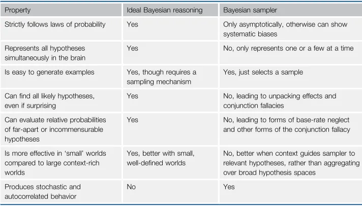
Bayesian sampler(seeGlossary). While the idea that cognition is implemented by Bayesian samplers is not new [18–27], here we show that any Bayesian sampler is faced with two challenges that automatically generate classic probabilistic reasoning errors, and only converge on‘well-behaved’probabilities at an (unattainable) limit of an infinite number of samples. In short, here we make the argument that Bayesian cognitive models that operate well in complex domains actually predict probabilistic reasoning errors in simple domains (seeTable 1, Key Table).

To see why, we begin with the well-known theoretical argument against the naïve conception that a Bayesian brain must represent all possible probabilities and make exact calculations using these probabilities: that such calculations are too complex for any physical system, including brains, to perform in even moderately complex domains[4,28–30]. A crude indication of this is that the number of real numbers required to encode the joint probability distribution overnbinary variables grows exponentially with 2n, quickly exceeding the capacity of any imaginable physical storage system. Yet Bayesian computational models often must represent vast data spaces, such as the space of possible images or speech waves; and effectively infinite hypothesis spaces, such as the space of possible scenes or sentences. Explicitly keeping track of

Trends

Bayesian models in cognitive science and artificial intelligence operate over domains such as vision, motor control and language processing by sampling from vastly complex probability distributions.

Such models cannot, and typically do not need to, calculate explicit probabilities.

Sampling naturally generates a variety of systematic probabilistic reasoning errors on elementary probability pro-blems, which are observed in experi-ments with people.

Thus, it is possible to reconcile prob-abilistic models of cognitive and brain function with the human struggle to master even the most elementary expli-cit probabilistic reasoning.

1

University of Warwick, Coventry, UK

2

Warwick Business School, Coventry, UK

*Correspondence:

[email protected]

probabilities in such complex domains such as vision and language, where Bayesian models have been most successful, is therefore clearly impossible.

Computational limits apply even in apparently simple cases. In a classic study, Tversky and Kahneman[31]asked people about the relative frequency of randomly choosing words thatfit the pattern _ _ _ _ _ n _ from a novel. An explicit Bayesian calculation would require three steps: (i) Posterior probabilities: calculating theposterior probabilitythat each of the tens of thousands of words in our vocabulary (and ideally over the 600 000 words in the Oxford English Dictionary) are found in a novel; (ii) Conditionalization:filtering those which fit the pattern _ _ _ _ _ n _; (iii) Marginalization: adding up the posterior probabilities of the words that passed thefilter to arrive at the overall probability that words randomly chosen from a novel wouldfit the pattern _ _ _ _ _ n _.

Explicitly performing these three steps is challenging, in terms of both memory and calculation; in more complex domains, each step is computationally infeasible. And the brain clearly does not do this: indeed, even the fact that a common word like‘nothing’fits the pattern is obvious only in retrospect[30].

How, then, can a Bayesian model of reading, speech recognition, or vision possibly work if it does not explicitly represent probabilities? A key insight is that, although explicitly representing and working with a probability distribution is hard, drawing samples from that distribution is relatively easy.Samplingdoes not require knowledge of the whole distribution. It can work merely with a local sense of relative posterior probabilities. Intuitively, we have this local sense: once we‘see’a solution (e.g.,‘nothing’), it is often easy to see that it is better than another solution (‘nothing’has higher posterior probability than‘capping’) even if we cannot exactly say what either posterior probability is. And now we have thought of two words ending in‘-ing’, we can rapidly generate more (sitting, singing, etc.). By continually sampling, we slowly build up a picture of all of the possibilities. Using a number of samples much smaller than the number of hypotheses makes the computations feasible.

Glossary

Ballistic accumulator model:a

model of evidence accumulation that explains both accuracy and response time. Unlike other similar models, it assumes that evidence accumulation is deterministic within each trial.

Base-rate neglect:a reasoning

fallacy in which individuals overweight diagnostic information (e.g., the fever I have could be caused by the Ebola virus) and underweight relevant background information (e.g., the Ebola virus is very rare).

Bayesian sampler:an

approximation to a Bayesian model that uses a sampling algorithm such as MCMC to avoid intractable integrals. While the model is used to perform Bayesian inference, the sampling algorithm itself is simply a mechanism for producing samples.

Boltzmann machine:an artificial

neural network with binary nodes that change state according to the

‘energy’of a pattern of states, or how well that patternfits the relationships determined by the edges between nodes.

Deep belief network:a hierarchical

artificial neural network of binary variables. Each layer of the network can be composed on simpler networks such as Boltzmann machines.

Markov chain Monte Carlo

(MCMC):a family of algorithms for

drawing samples from probability distributions. These algorithms transition from state to state with probabilities that depend only on the current state. The transition probabilities are carefully chosen so that the states are (dependent) samples of a target probability distribution.

Metropolis–Hastings:An MCMC

algorithm that proposes new states based on the current state, and transitions to new states based on the relative probability of the current state and the proposed state.

Multistable stimuli:stimuli with

more than one perceptual interpretation. One's perception of the stimulus tends to switch back and forth between interpretations over time.

Normalization constant:while

probabilities of all of the hypotheses must sum to 1, often it is much easier to represent values that are proportional to the probabilities instead. The normalizing constant is Key Table

Table 1. Properties of a Bayesian Sampler Compared to Ideal

Bayesian Reasoning

Property Ideal Bayesian reasoning Bayesian sampler

Strictly follows laws of probability Yes Only asymptotically, otherwise can show systematic biases

Represents all hypotheses simultaneously in the brain

Yes No, only represents one or a few at a time

Is easy to generate examples Yes, though requires a sampling mechanism

Yes, just selects a sample

Canfind all likely hypotheses, even if surprising

Yes No, leading to unpacking effects and conjunction fallacies

Can evaluate relative probabilities of far-apart or incommensurable hypotheses

Yes No, leading to forms of base-rate neglect and other forms of the conjunction fallacy

Is more effective in‘small’worlds compared to large context-rich worlds

Yes, better with small, well-defined worlds

No, better when context guides sampler to relevant hypotheses, rather than aggregating over broad hypothesis spaces

Produces stochastic and autocorrelated behavior

the sum of these proportional values

–it is the number by which each of these proportional values must be divided to become probabilities.

Particlefilters:an algorithm

designed to sample from probability distributions for data that arrives sequentially.

Posterior probability:the probability

of a hypothesis in response to a question.

Sampling:generating hypotheses

with frequency proportional to their posterior probability. Probability estimates can then be based on the relative frequencies of these sampled hypotheses.

Satisficing:searching until a

good-enough solution is found, rather than searching until the best possible solution is found.

Small worlds:restricted worlds with

few variables and well-defined probabilities over those variables.

Wisdom of crowds:empirical result

that the aggregation of individual estimates is better than the average individual estimate, or sometimes any individual estimate.

This sampling approach to probabilistic inference began in the 1940s and 1950s[32,33]; and is ubiquitously and successfully applied in complex cognitive domains, whether cognitive science or artificial intelligence[5,34]. If we sample forever, we can make any probabilistic estimate we need to, without ever calculating explicit probabilities. But, as we shall see, restricted sampling will instead lead to systematic probabilistic errors–including some classic probabilistic reason-ing fallacies.

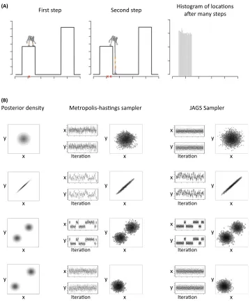
So how does this work in practice? Think of a posterior probability distribution as a hilly high-dimensional landscape over possible hypotheses (seeFigure 1A). Knowing the shape of this landscape, and even its highest peaks, is impossibly difficult. But a sampling algorithm simply explores the landscape, step by step. Perhaps the best known class of sampling algorithms is

Markov chain Monte Carlo(MCMC[35,36]). A common type of MCMC, theMetropolis– Hastingsalgorithm[32,37], can be thought of as an android trying to climb the peaks of the probability distribution, but in dense fog, and with no memory of where it has been. It climbs by sticking one foot out in a random direction and‘noisily’judging whether it is moving uphill (i.e., it noisily knows a ‘better’hypothesis when it finds one). If so, it shifts to the new location; otherwise, it stays put. The android repeats the process, slowly climbing through the probability landscape, using only the relative instead of absolute probability to guide its actions.

Despite the simplicity of the android's method, a histogram of the android's locations will resemble the hill (arbitrarily closely, in the limit), meaning the positions are samples from the probability distribution (see last column ofFigure 1A). These samples can then easily be used in a variety of calculations. For example, to estimate the chance that a word in a novel will follow the form _ _ _ _ _ n_, just sample some text, and use the proportion of the samples that follow that pattern as the estimate. This is, indeed, very close to Tversky and Kahneman's availability heuristic[38]–to work out how likely something is by generating possible examples; but now construed as Bayesian sampling rather than a mere‘rule of thumb.’

There is powerful prima facie evidence that the brain can readily draw samples from very complex distributions. We can imagine visual or auditory events, and we can generate language (and most tellingly to mimic the language, gestures, or movements of other people), which are forms of sampling[39]. Similarly, when given a part of a sentence, or fragments of a picture, people generate one (and sometimes many) possible completions[40,41]. This‘generative’ aspect of perception and cognition (e.g.,[42]) follows automatically from sampling models [6,10].

Unavoidable Limitations of Sampling

Any distribution that can be sampled can, in the limit, be approximated–butfinite samples will be imperfect and hence potentially misleading. The android's progress around the probability landscape is,first and most obviously, biased by its starting point. Suppose, specifically, that the landscape contains an isolated peak. Starting far from the peak in an undulating landscape, the android has little chance offinding the peak. Even complex sampling algorithms, that can be likened to more advanced androids that sense the gradient under their feet or are adapted to particular landscapes, will blindly search in the foothills, missing the mountain next door (see Figure 1A and bottom row ofFigure 1B). While we have illustrated this problem with a simple sampling algorithm, it applies to any sampling algorithm without prior knowledge of the location of the peaks[28,30]; indeed even the inventors of sampling algorithms are not immune to these problems[36,43].

(B) (A)

First step

Posterior density Metropolis-hasngs sampler

Iteraon

Iteraon

Iteraon

Iteraon Iteraon

Iteraon Iteraon Iteraon

JAGS Sampler Second step Histogram of locaons

aer many steps

y x

y x

y x

y x

y x

y x y

x

y x

y x y

x

y x

y

y x

x

y x y x y x y x

y x y x y x

same event, violating probability theory. In the unpacking effect, participants judge, say,‘being a lawyer’, to be less probable than the‘unpacked’description‘being a tax, corporate, patent, or other type of lawyer’[44–46]. From a sampling point of view, bringing to mind types of lawyer that are numerous but of low salience ensures these ‘peaks’ are not missed by the sampling process, yielding a higher probability rating. Yet unpacking can also guide people away from the high probability hypotheses: if the unpacked hypotheses are low probability instead of high, for example trying to assess whether a person with a background in social activism becomes either‘a lawyer’or‘a tax, corporate, patent, or other type of lawyer’then the probability of the unpacked event is judged less than that of the packed event[46]–the sampler is guided away from the peaks of probability (e.g.,‘human rights lawyer’).

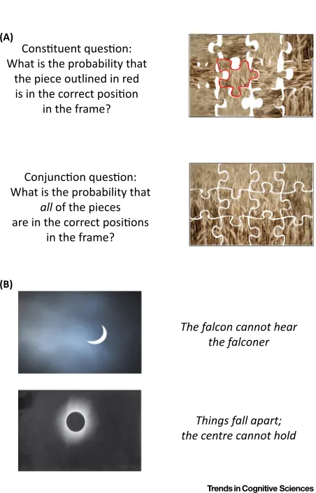
The conjunction fallacy is a complex effect[47,48], but one source of the fallacy is the inability to bring to mind relevant information. We struggle to estimate how likely a random word in a novel will match the less detailed pattern _ _ _ _ _ n _: our sampling algorithm searches around a large space and may miss peaks of high probability. However, when guided to where the peaks are (i.e., starting the android from a different location), for example, by being asked about the pattern _ _ _ _ ing in the more detailed description, then large peaks are found and probability estimates are higher[31,45]. The process involved is visually illustrated inFigure 2A. The conjunction of the correct locations of all the puzzle pieces cannot, of course, be more probable that the correct location of a single piece. Yet when considered in isolation, the evidence that an isolated piece is correct is weak (from a sampling standpoint, it is not clear whether, e.g., swapping pieces leads to a higher or lower probability). But in the fully assembled puzzle (i.e., the‘peak’in probability space is presented), local comparisons are easy–switching any of the pieces would make thefit worse–so you can be nearly certain that all the pieces are in the correct position. So the whole puzzle will be judged more probable than a single piece, exhibiting the conjunction fallacy.

A second bias in sampling is subtler. Sometimes regions of high probability are so far apart that a sampler starting in one region is extremely unlikely to transition to the other. As shown in Figure 2B, our android could be set down in Britain or in Colorado, and in each case would gradually build up a picture of the local topography. But these local topographies would give no clue that the baseline height of Colorado is much higher than Britain. The android is incredibly unlikely to wander from one region to another so the relative heights of the two regions would remain unknown.

This problem is not restricted to sampling algorithms or to modes that are far apart in a single probability distribution. Indeed, the problem is even starker when a Bayesian sampler compares probabilities in entirely different models–then it is often extremely difficult for the android to shuttle between landscapes[49]. So, for example, although it is obvious that we are more likely to obtain at least one, rather than at leastfive, double sixes from 24 dice throws, it is by no means obvious whether thisfirst event is more or less likely than obtaining heads in a coinflip. Indeed, this problem sparked key developments in early probability theory by Pascal and Fermat[50].

One might think there is an easy solution to comparing across domains. Probabilities must sum to 1, after all. So if sampling explores the entire landscape, then we canfigure out the absolute size of probabilities (i.e., whether we are dealing with Britain or Colorado) because the volume under the landscape must be precisely 1. But exploring the entire landscape is impossible– because the space is huge and may contain unknown isolated peaks of any possible size, as we’ve seen (technically, the normalization constant often cannot be determined, even approximately).

eclipse; or which of two quotations are more likely to appear on a randomly chosen website. However, between-domain comparisons, such as deciding whether a total eclipse is more likely than‘Things fall apart; the centre cannot hold’appearing is more difficult: the astronomical event and the quotation must be compared against different sets of experiences (e.g., years and websites, respectively).

Being unable to effectively compare the probabilities of two hypotheses is a second way in which a Bayesian sampler generates reasoning fallacies observed in people. The example inFigure 2B also illustrates a version ofbase-rate neglect.‘Things fall apart; the centre cannot hold’is a notable quotation, and eclipses are rare, so from local comparisons it may seem that‘Things fall apart; the centre cannot hold’is more likely. However, the base rates, which are often neglected, reverse this: the vast majority of websites have no literary quotations, and each year provides many opportunities for an eclipse. Fully taking account of base-rates would require searching the entire probability space–which is typically impossible. This inability to compare probabilities from different domains plays a role in other reasoning fallacies: the conjunction fallacy also

(A)

(B)

Constuent queson: What is the probability that

the piece outlined in red is in the correct posion

in the frame?

Conjuncon queson: What is the probability that

all of the pieces are in the correct posions

in the frame?

The falcon cannot hear the falconer

Things fall apart; the centre cannot hold

occurs when the two conjoined events are completely unrelated to one another[51]. While a sampler can provide a rough sense of the probabilities of each hypothesis separately (is this quotation or astronomical event common compared with similar quotes or astronomical events), the inability to bridge between the two phenomena means that sampling cannot accurately assess base rates or estimate the probabilities of conjunctions or disjunctions. In these cases, participants are left to combine the non-normalized sampled probability estimates for each hypothesis‘manually’, and perhaps choose just one of the probabilities or perhaps combine them inappropriately[52–54].

Interestingly, accuracy is improved in base-rate neglect studies when a causal link is provided between the individual events[55,56], and experiencing outcomes together weakens conjunc-tion fallacies[57]–we can interpret these studies as providing a link that allows a Bayesian sampler to traverse between the two regions to combine probabilities meaningfully.

Sampling and Task Richness

Reasoning fallacies such as the unpacking effect, conjunction fallacy, and base-rate neglect have greatly influenced our general understanding of human cognition. They arise in very simple situations and violate the most elementary laws of probability. We agree that these fallacies make a convincing argument against the view that the brain represents and calculates probabilities directly.

This argument appears strengthened in complex real-world tasks. If our brains do not respect the laws of probability for simple tasks, surely the Bayesian approach to the mind must fail in rich domains such as vision, language and motor control with huge data and hypothesis spaces[29]. Indeed, even Savage, the great Bayesian pioneer, suggested restricting Bayesian methods to

‘small’worlds[58,59].

Viewing brains as sampling from complex probability distributions upends this argument. Rich, realistic tasks, in which there is a lot of contextual information available to guide sampling, are just those where the Bayesian sampler is most effective. Rich tasks focus the sampler on the areas of the probability landscape that matter–those that arise through experience. By limiting the region in which the sampler must search, rich problems can often be far easier for the sampler than apparently simpler, but more abstract, problems. Consider how hard it would be to solve a jigsaw which is uniformly white; the greater the richness of the picture on the jigsaw, the more the sampler can locally be guided by our knowledge of real-world scenes.

For these reasons, Bayesian models of cognition have primarilyflourished as explanations of the complex dependency of behavior on the environment in domains including intuitive physics, causal learning, perception, motor control, and language [1–10]; and these computational models generally do not involve explicit probability calculations, but apply Bayesian sampling, using methods such as MCMC.

We have argued that rich real-world tasks may be more tractable to Bayesian sampling than abstract lab tasks, because sampling is more constrained. But is it possible that the fundamental difference is not task richness, but cognitive architecture, for example, between well-optimized Bayesian perceptual processes and heuristic central processes[63,64]? We do not believe this to be the case for two reasons. First, the differences between these kinds of tasks tendsdiffer-ence between these kinds of tasks tends to disappear when performance is measured on the same scale[65,66]. Second, there are counterexamples to the architectural distinction. Lan-guage interpretation is a high-level cognitive task which shows a good correspondence to Bayesian models[5,6]. And, conversely, purely perceptual versions of reasoning fallacies can be constructed, asFigure 2A illustrates. More broadly, any perceptual task where a hint can disambiguate the stimulus (e.g., sine-wave speech[67]) will generate examples of the conjunc-tion fallacy.

If the brain is indeed a Bayesian sampler, then sampling should leave traces in behavior. One immediate consequence is that behavior should be stochastic, because of the variability of the samples drawn. Hence behavior will look noisy, even where on average the response will be correct (e.g., generating thewisdom of crowdseven from a single individual[68–70]). The ubiquitous variability of human behavior, especially in highly abstract judgments or choice tasks [71–74]is puzzling for pure‘optimality’explanations. Bayesian samplers can match behavioral stochasticity in tasks such as perception, categorization, causal reasoning, and decision making [20,21,23,24].

A second consequence of sampling is that behavior will be autocorrelated, meaning that each new sample depends on the last, because the sampler makes only small steps in the probability landscape (seeBox 1). Autocorrelation appears ubiquitous within and between trials throughout memory, decision making, perception, language, and motor control (e.g.,[75,76]), and Bayesian samplers produce human-like autocorrelations in perceptual and reasoning tasks[18,25]. One

Box 1. Sampling and Autocorrelation

When sampling from complex distributions, it is often impossible to draw samples directly, and sampling algorithms such as MCMC are used instead. Because these algorithms look locally when producing the next sample, autocorrelation can result.Figure 1B[3_TD$DIFF]in main text compares samples drawn independently to samples drawn from two versions of MCMC: the Metropolis–Hastings algorithm and Gibbs sampling as implemented in JAGS[36,93]. Samples produced by both MCMC methods have low autocorrelations for independent unimodal distributions (top row ofFigure 1B), but for highly correlated variables and bimodal distributions autocorrelations are more prevalent, even when the aggregated samples match the overall distribution (middle rows ofFigure 1B). More recently developed sampling methods such as those employed by the program Stan can also show sample autocorrelations, but more complex distributions are needed to induce them[94]. And of course, when two modes are far apart, these samplers are very unlikely to sample both modes (bottom row ofFigure 1B).

Although they are outnumbered by models of behavior that assume independent sampling, several models of memory and decision making do assume there are autocorrelations in sampling. Models of free recall such as Search of Associative Memory[95]and SIMPLE[96]use the previously recalled word to cue the next word, and has been productively used to account for the dependencies seen when people attempt to recall a list of words. In decision making,

theballistic accumulator modelcould be considered an extreme version of autocorrelation in which each internal time

step produces the same strength of sampled evidence within a trial[97]. Explicit models of autocorrelated sampling have been used to account for perceptual switching times ofmultistable stimuli[18]and anchoring effects in reasoning tasks

particular consequence of autocorrelation will be that‘priming’a particular starting point in the sampling process will bias the sampler. Thus, asking, for example, the gestation time of an elephant will bias a person's estimate because they begin with the common reference point of 9 months: the starting point is an ‘anchor’ and sampling ‘adjusts’ from that anchor – but insufficiently when small samples are drawn. This provides a Bayesian reinterpretation of

‘anchoring and adjustment’[25], a process widely observed in human judgment[15,77].

The extent of autocorrelation depends on both the algorithm and the probability distribution (see Figure 1B). Sampling algorithms often have tuning parameters which are chosen to minimize autocorrelation and to better explore multiple peaks. Of course the best settings of these tuning parameters are not known in advance, but they can be learned by drawing‘warm-up’samples to get a sense of what the distribution is like. Interestingly, there is behavioral evidence for this. Participants given‘clumpier’reward distributions in a 2D computer foraging task later behaved as if ‘tuned’ to clumpier distributions in semantic space in a word-generations task. This suggests that there is a general sampling process that people adapt to the properties of the probability distributions that they face[78–80].

Concluding Remarks and Future Perspectives

Sampling provides a natural and scalable implementation of Bayesian models. Moreover, the questions that are difficult to answer with sampling correspond to those with which people struggle, and those easier to answer with sampling are contextually rich, and highly complex, real-world questions on which people show surprising competence. Sampling generates reasoning fallacies, and leaves traces, such as stochasticity and autocorrelations, which are observed in human behavior.

The sampling viewpoint alsofits with current thinking in computational neuroscience, where an influential proposal is that transitions between brain states correspond to sampling from a probability distribution[26,27,81,82]or multiple samples are represented simultaneously (e.g., usingparticlefilters[83–86]).

Moreover, neural networks dating back to theBoltzmann machine [87]take a sampling approach to probabilistic inference. For example, consider deep belief networks, which have been highly successful in vision, acoustic analysis, language, and other areas of machine learning[88]. These networks consist of layers of binary variables connected by weights. Once the network is trained, it defines a probability distribution over the output features. However, the probabilities of configurations of output features are not known. Instead, samples from the total probability distribution are generated by randomly initializing the output variables; and conditional samples are generated byfixing some of the output variables to particular values and sampling the remaining variables. Applications of deep belief networks include generating facial expressions and recognizing objects[34,89]. As with human performance, these net-works readily sample highly complex probability distributions, but can only calculate explicit probabilities with difficulty. Of course, it is possible that the brain represents probability distributions over small collections of variables[90,91], or variational approximations to prob-ability distributions[92], but this would not affect our key argument, which stems from the unavoidable difficulty of finding isolated peaks in, and calculating the volume of, complex probability distributions.

While Bayesian sampling has great promise in answering the big questions of how Bayesian cognition could work, there are many open issues. As detailed in Outstanding Questions, interesting avenues for future work are computational models of reasoning fallacies, explan-ations of how complex causal structures are represented, and further exploration of the nature of the sampling algorithms that may be implemented in the mind and the brain.

Outstanding Questions Is sampling sequential or parallel? If the brain samples distributed patterns across a network of neurons (in line with connectionist models), then sam-pling should be sequential. This implies severe attentional limitations: for exam-ple, that we can sample from, recog-nize, or search for, one pattern at a time.

How is sampling neurally implemented? Connectionist models suggest that sampling may be implemented naturally across a distributed network, such as the brain.

How are‘autocorrelated’samples inte-grated by the brain? Accumulator models in perception, categorization, and memory seem best justified if sam-pling is independent. How should such models and their predictions be recast in the light of autocorrelated samples?

Does autocorrelation of samples reduce over trials as the brain becomes tuned to particular tasks?

Are samples drawn from the correct complex probability distribution or is the distribution simplified first? Varia-tional approximations can be used to simplify complex probability distribu-tions at the cost of a loss of accuracy.

How does sampling deal with counter-factuals and the arrow of causality? Does sampling across causal networks allow us to‘imagine’what might have happened if Hitler had been assassi-nated in 1934? How can we sample over entirelyfictional worlds (e.g., to consider possible endings to a story)?

How far can we simulate sampling in

‘other minds’to infer what other people are thinking?

How are past interpretations sup-pressed to generate new interpreta-tions for ambiguous stimuli?

Acknowledgments

ANS was supported by the ESRC (grant number ES/K004948/1). NC was supported by ERC grant 295917-RATIONALITY, the ESRC Network for Integrated Behavioural Science (grant number ES/K002201/1), the Leverhulme Trust (grant number RP2012-V-022), RCUK Grant EP/K039830/1.

[4_TD$DIFF]

Supplemental[5_TD$DIFF]Information

Supplemental information associated with this article can be found, in the online version, athttp://dx.doi.org/10.1016/j.tics.

2016.10.003.

References

1. Battaglia, P.W. et al. (2013) Simulation as an engine of physical scene understanding.Proc. Natl. Acad. Sci. U.S.A.

110, 18327–18332

2. Sanborn, A.N.et al.(2013) Reconciling intuitive physics and New-tonian mechanics for colliding objects.Psychol. Rev.120, 411

3. Pantelis, P.C.et al.(2014) Inferring the intentional states of auton-omous virtual agents.Cognition130, 360–379

4. Anderson, J.R. (1991) The adaptive nature of human categoriza-tion.Psychol. Rev.98, 409

5. Griffiths, T.L.et al.(2007) Topics in semantic representation.

Psychol. Rev.114, 211

6. Chater, N. and Manning, C.D. (2006) Probabilistic models of language processing and acquisition.Trends Cogn. Sci.10, 335–344

7. Goodman, N.D.et al.(2008) A rational analysis of rule-based concept learning.Cogn. Sci.32, 108–154

8. Kemp, C. and Tenenbaum, J.B. (2009) Structured statistical mod-els of inductive reasoning.Psychol. Rev.116, 20–58

9. Wolpert, D.M. (2007) Probabilistic models in human sensorimotor control.Hum. Mov. Sci.26, 511–524

10.Yuille, A. and Kersten, D. (2006) Vision as Bayesian inference: analysis by synthesis?Trends Cogn. Sci.10, 301–308

11.Houlsby, N.M.T.et al.(2013) Cognitive tomography reveals com-plex, task-independent mental representations.Curr. Biol.23, 2169–2175

12.Griffiths, T.L. and Tenenbaum, J.B. (2011) Predicting the future as Bayesian inference: people combine prior knowledge with obser-vations when estimating duration and extent.J. Exp. Psychol. Gen.140, 725

13.Petzschner, F.H.et al.(2015) A Bayesian perspective on magni-tude estimation.Trends Cogn. Sci.19, 285–293

14.Brighton, H. and Gigerenzer, G. (2012) Are rational actor models

‘rational’outside small worlds. InEvolution and Rationality: Deci-sions, Co-operation, and Strategic Behavior(Okasha, S. and Binmore, K., eds), pp. 84–109, Cambridge, NY, Cambridge Uni-versity Press

15.Tversky, A. and Kahneman, D. (1974) Judgment under uncer-tainty: heuristics and biases.Science185, 1124–1131

16.Elqayam, S. and Evans, J.S.B. (2011) Subtracting‘ought’from‘is’: descriptivism versus normativism in the study of human thinking.

Behav. Brain Sci.34, 233–248

17.Gigerenzer, G. and Gaissmaier, W. (2011) Heuristic decision mak-ing.Annu. Rev. Psychol.62, 451–482

18.Gershman, S.J.et al.(2012) Multistability and perceptual infer-ence.Neural Comput.24, 1–24

19.Griffiths, T.L.et al.(2012) Bridging levels of analysis for probabi-listic models of cognition.Curr. Directions Psychol. Sci.21, 263–268

20.Vul, E.et al.(2014) One and done? Optimal decisions from very few samples.Cogn. Sci.38, 599–637

21.Sanborn, A.N.et al.(2010) Rational approximations to rational models: alternative algorithms for category learning.Psychol. Rev.

117, 1144

22.Shi, L.et al.(2010) Exemplar models as a mechanism for perform-ing Bayesian inference.Psychon. Bull. Rev.17, 443–464

23.Wozny, D.R.et al.(2010) Probability matching as a computa-tional strategy used in perception. PLoS Comput. Biol.6, e1000871

24.Denison, S.et al.(2013) Rational variability in children's causal inferences: the sampling hypothesis.Cognition126, 285–300

25.Lieder, F.et al.(2012) Burn-in, bias, and the rationality of anchor-ing.Adv. Neural Inf. Process Syst.25, 2690–2798

26.Fiser, J.et al.(2010) Statistically optimal perception and learning: from behavior to neural representations.Trends Cogn. Sci.14, 119–130

27.Moreno-Bote, R.et al.(2011) Bayesian sampling in visual percep-tion.Proc. Natl. Acad. Sci. U.S.A.108, 12491–12496

28.Kwisthout, J.et al.(2011) Bayesian intractability is not an ailment that approximation can cure.Cogn. Sci.35, 779–784

29.Gigerenzer, G. and Goldstein, D.G. (1996) Reasoning the fast and frugal way: models of bounded rationality.Psychol. Rev.103, 650

30.Aragones, E.et al.(2005) Fact-free learning.Am. Econ. Rev.95, 1355–1368

31.Tversky, A. and Kahneman, D. (1983) Extensional versus intuitive reasoning: the conjunction fallacy in probability judgment.Psychol. Rev.90, 293

32.Metropolis, N.et al.(1953) Equation of state calculations by fast computing machines.J. Chem. Phys.21, 1087–1092

33.Metropolis, N. and Ulam, S. (1949) The Monte Carlo method.J. Am. Stat. Assoc.44, 335–341

34.Susskind, J.M.et al.(2008) Generating facial expressions with deep belief nets. InAffective Computing, Emotion Modelling, Synthesis and Recognition(Kordic, V., ed.), pp. 421–440, ARS Publishers

35.Neal, R.M. (1993)Probabilistic inference using Markov chain Monte Carlo methods.

36.Geman, S. and Geman, D. (1984) Stochastic relaxation, Gibbs distributions, and the Bayesian restoration of images.IEEE Trans. Pattern Anal. Mach. Intell.6, 721–741

37.Hastings, W.K. (1970) Monte Carlo sampling methods using Mar-kov chains and their applications.Biometrika57, 97–109

38.Tversky, A. and Kahneman, D. (1973) Availability: a heuristic for judging frequency and probability.Cogn. Psychol.5, 207–232

39.Griffiths, T.L. and Kalish, M.L. (2007) Language evolution by iterated learning with Bayesian agents.Cogn. Sci.31, 441–480

40.Bloom, P.A. and Fischler, I. (1980) Completion norms for 329 sentence contexts.Mem. Cogn.8, 631–642

41.Gold, J.M.et al.(2000) Deriving behavioural receptivefields for visually completed contours.Curr. Biol.10, 663–666

42.Shepard, R.N. (1984) Ecological constraints on internal represen-tation: resonant kinematics of perceiving, imagining, thinking, and dreaming.Psychol. Rev.91, 417

43.Morris, R.et al.(1996) The Ising/Potts model is not well suited to segmentation tasks. InDigital Signal Processing Workshop Pro-ceedings, 1996, IEEE, pp. 263–266, IEEE

44.Fischhoff, B.et al.(1978) Fault trees: sensitivity of estimated failure probabilities to problem representation.J. Exp. Psychol. Hum. Percept. Perform.4, 330

45.Tversky, A. and Koehler, D.J. (1994) Support theory: a nonexten-sional representation of subjective probability.Psychol. Rev.101, 547

46.Sloman, S.et al.(2004) Typical versus atypical unpacking and superadditive probability judgment.J. Exp. Psychol. Learn. Mem. Cogn.30, 573–582

47.Hertwig, R. and Gigerenzer, G. (1999) The‘conjunction fallacy’

48.Wedell, D.H. and Moro, R. (2008) Testing boundary conditions for the conjunction fallacy: effects of response mode, conceptual focus, and problem type.Cognition107, 105–136

49.Han, C. and Carlin, B.P. (2001) Markov chain Monte Carlo meth-ods for computing Bayes factors.J. Am. Stat. Assoc.96, 1122–

1132

50.David, F.N. (1998)Games, Gods, and Gambling: A History of Probability and Statistical Ideas,Courier Corporation

51.Gavanski, I. and Roskos-Ewoldsen, D.R. (1991) Representative-ness and conjoint probability.J. Pers. Soc. Psychol.61, 181

52.Cosmides, L. and Tooby, J. (1996) Are humans good intuitive statisticians after all? Rethinking some conclusions from the liter-ature on judgment under uncertainty.Cognition58, 1–73

53.Fisk, J.E. (2002) Judgments under uncertainty: representativeness or potential surprise?Br. J. Psychol.93, 431–449

54.Nilsson, H.et al.(2009) Linda is not a bearded lady: configural weighting and adding as the cause of extension errors.J. Exp. Psychol. Gen.138, 517

55.Ajzen, I. (1977) Intuitive theories of events and the effects of base-rate information on prediction.J. Pers. Soc. Psychol.35, 303

56.Krynski, T.R. and Tenenbaum, J.B. (2007) The role of causality in judgment under uncertainty.J. Exp. Psychol. Gen.136, 430

57.Nilsson, H. (2008) Exploring the conjunction fallacy within a cate-gory learning framework.J. Behav. Decis. Mak.21, 471–490

58.Binmore, K. (2008)Rational Decisions,Princeton University Press

59.Savage, L.J. (1954)The Foundations of Statistics,Wiley

60.McGurk, H. and MacDonald, J. (1976) Hearing lips and seeing voices.Nature264, 746–748

61.Marr, D. (1982)Vision,W.H. Freeman

62.Simon, H.A. (1956) Rational choice and the structure of the environment.Psychol. Rev.63, 129

63.Maloney, L.T.et al.(2007) Questions without words: a comparison between decision making under risk and movement planning under risk.Integrated Models Cogn. Syst.297–313

64.Oaksford, M. and Hall, S. (2016) On the source of human irratio-nality.Trends Cogn. Sci.20, 336–344

65.Jarvstad, A.et al.(2013) Perceptuo-motor, cognitive, and descrip-tion-based decision-making seem equally good.Proc. Natl. Acad. Sci. U.S.A.110, 16271–16276

66.Jarvstad, A.et al.(2014) Are perceptuo-motor decisions really more optimal than cognitive decisions?Cognition130, 397–416

67.Remez, R.E.et al.(1981) Speech perception without traditional speech cues.Science212, 947–949

68.Vul, E. and Pashler, H. (2008) Measuring the crowd within proba-bilistic representations within individuals.Psychol. Sci.19, 645–

647

69.Stroop, J.R. (1932) Is the judgment of the group better than that of the average member of the group?J. Exp. Psychol.15, 550

70.Herzog, S.M. and Hertwig, R. (2014) Harnessing the wisdom of the inner crowd.Trends Cogn. Sci.18, 504–506

71.Mosteller, F. and Nogee, P. (1951) An experimental measurement of utility.J. Polit. Econ.59, 371–404

72.Loomes, G. (2015) Variability, noise, and error in decision making under risk. InThe Wiley Blackwell Handbook of Judgment and Decision Making(Keren, G. and Wu, G., eds), pp. 658–695, Wiley

73.Herrnstein, R.J. (1961) Relative and absolute strength of response as a function of frequency of reinforcement.J. Exp. Anal. Behav.4, 267–272

74.Vulkan, N. (2000) An economist's perspective on probability matching.J. Econ. Surveys14, 101–118

75.Gilden, D.L.et al.(1995) 1/f noise in human cognition.Science

267, 1837

76.Kello, C.T.et al.(2008) The pervasiveness of 1/f scaling in speech reflects the metastable basis of cognition.Cogn. Sci.32, 1217–1231

77.Epley, N. and Gilovich, T. (2006) The anchoring-and-adjustment heuristic: why the adjustments are insufficient.Psychol. Sci.17, 311–318

78.Abbott, J.T.et al.(2015) Random walks on semantic networks can resemble optimal foraging.Psychol. Rev.122, 558–559

79.Hills, T.T.et al.(2012) Optimal foraging in semantic memory.

Psychol. Rev.119, 431

80.Hills, T.T.et al.(2008) Search in external and internal spaces evidence for generalized cognitive search processes.Psychol. Sci.19, 802–808

81.Hennequin, G.et al.(2014) Fast sampling-based inference in balanced neuronal networks.Adv. Neural Inf. Process Syst.27, 2240–2248

82.Buesing, L.et al.(2011) Neural dynamics as sampling: a model for stochastic computation in recurrent networks of spiking neurons.

PLoS Comput. Biol.7, e1002211

83.Lee, T.S. and Mumford, D. (2003) Hierarchical Bayesian inference in the visual cortex.J. Opt. Soc. Am. A. Opt. Image Sci. Vis.20, 1434–1448

84.Huang, Y. and Rao, R.P. (2014) Neurons as Monte Carlo sam-plers: Bayesian inference and learning in spiking networks.Adv. Neural Inf. Process Syst.27, 1943–1951

85.Legenstein, R. and Maass, W. (2014) Ensembles of spiking neu-rons with noise support optimal probabilistic inference in a dynam-ically changing environment.PLoS Comput. Biol.10, e1003859

86.Probst, D.et al.(2015) Probabilistic inference in discrete spaces can be implemented into networks of LIF neurons.Front. Comput. Neurosci.9, 13

87.Ackley, D.H.et al.(1985) A learning algorithm for Boltzmann machines.Cogn. Sci.9, 147–169

88.Hinton, G.E.et al.(2006) A fast learning algorithm for deep belief nets.Neural Comput.18, 1527–1554

89.Nair, V. and Hinton, G.E. (2009) 3D object recognition with deep belief nets.Adv. Neural Inf. Process Syst.22, 1339–1347

90.Kopp, B.et al.(2016) P300 amplitude variations, prior probabili-ties, and likelihoods: a Bayesian ERP study.Cogn. Affect. Behav. Neurosci.16, 911–928

91.Chan, S.C.Y.et al.(2016) A probability distribution over latent causes in the orbitofrontal cortex.J. Neurosci.36, 7817–7828

92.Friston, K. (2008) Hierarchical models in the brain.PLoS Comput. Biol.4, e1000211

93.Plummer, M. (2003) JAGS: a program for analysis of Bayesian graphical models using Gibbs sampling. InProceedings of the 3rd International Workshop on Distributed Statistical Computing, pp. 125

94.Carpenter, B.et al.(2016) Stan: a probabilistic programming language.J. Stat. Softw.

95.Raaijmakers, J.G. and Shiffrin, R.M. (1981) Search of associative memory.Psychol. Rev.88, 93

96.Brown, G.D.et al.(2007) A temporal ratio model of memory.

Psychol. Rev.114, 539