Operation and performance of the ATLAS semiconductor tracker

Original citation:

ATLAS Collaboration (Including: Farrington, Sinead, Harrison, P. F., Janus, M., Jeske, C., Jones, G. (Graham), Martin, T. A., Murray, W. and Pianori, E.). (2014) Operation and performance of the ATLAS semiconductor tracker. Journal of Instrumentation, Volume 9 . Article number P08009 .

Permanent WRAP url:

http://wrap.warwick.ac.uk/63695

Copyright and reuse:

The Warwick Research Archive Portal (WRAP) makes this work of researchers of the University of Warwick available open access under the following conditions.

This article is made available under the Creative Commons Attribution- 3.0 Unported (CC BY 3.0) license and may be reused according to the conditions of the license. For more details seehttp://creativecommons.org/licenses/by/3.0/

A note on versions:

The version presented in WRAP is the published version, or, version of record, and may be cited as it appears here.

This content has been downloaded from IOPscience. Please scroll down to see the full text.

Download details:

IP Address: 137.205.202.97

This content was downloaded on 29/10/2014 at 15:38

Please note that terms and conditions apply.

Operation and performance of the ATLAS semiconductor tracker

View the table of contents for this issue, or go to the journal homepage for more 2014 JINST 9 P08009

(http://iopscience.iop.org/1748-0221/9/08/P08009)

2014 JINST 9 P08009

RECEIVED:April 29, 2014

REVISED:May 6, 2014

ACCEPTED:July 7, 2014

PUBLISHED:August 27, 2014

Operation and performance of the ATLAS

semiconductor tracker

The ATLAS collaboration

E-mail:atlas.publications@cern.ch

ABSTRACT: The semiconductor tracker is a silicon microstrip detector forming part of the inner tracking system of the ATLAS experiment at the LHC. The operation and performance of the semiconductor tracker during the first years of LHC running are described. More than 99% of the detector modules were operational during this period, with an average intrinsic hit efficiency of (99.74±0.04)%. The evolution of the noise occupancy is discussed, and measurements of the Lorentz angle,δ-ray production and energy loss presented. The alignment of the detector is found to be stable at the few-micron level over long periods of time. Radiation damage measurements, which include the evolution of detector leakage currents, are found to be consistent with predictions and are used in the verification of radiation background simulations.

KEYWORDS: Solid state detectors; Charge transport and multiplication in solid media; Particle tracking detectors (Solid-state detectors); Detector modelling and simulations I (interaction of ra-diation with matter, interaction of photons with matter, interaction of hadrons with matter, etc)

2014 JINST 9 P08009

Contents

1 Introduction 1

2 The SCT detector 3

2.1 Layout and modules 3

2.2 Readout and data acquisition system 4

2.3 Detector services and control system 6

2.4 Frequency scanning interferometry 7

2.5 Detector safety 9

3 Operation 9

3.1 Detector status 10

3.2 Calibration 12

3.3 Timing 12

3.4 Data-taking efficiency 13

3.5 Operations issues 14

4 Offline reconstruction and simulation 15

4.1 Track reconstruction 15

4.2 Track alignment 17

4.3 Simulation 18

4.3.1 Digitisation model 18

4.3.2 Induced-charge model 19

4.4 Conditions data 19

5 Monitoring and data quality assessment 20

5.1 Online monitoring 20

5.2 Offline monitoring 21

5.3 Data quality assessment 21

5.4 Prompt calibration loop 22

6 Performance 23

6.1 Detector occupancy 23

6.2 Noise 26

6.3 Alignment stability 28

6.4 Intrinsic hit efficiency 31

6.5 Lorentz angle 34

6.6 Energy loss and particle identification 38

2014 JINST 9 P08009

7 Radiation effects 41

7.1 Simulations and predictions 43

7.2 Detector leakage currents 44

7.2.1 Temperature and leakage-current measurement 45 7.2.2 Leakage-current evolution and comparison with predictions 45

7.3 Online radiation monitor measurements 46

7.4 Single-event upsets 48

7.5 Impact of radiation on detector operation and its mitigation 49

8 Conclusions 51

A Estimation of the bulk leakage current using models 52

The ATLAS collaboration 57

1 Introduction

The ATLAS detector [1] is a multi-purpose apparatus designed to study a wide range of physics processes at the Large Hadron Collider (LHC) [2] at CERN. In addition to measurements of Stan-dard Model processes such as vector-boson and top-quark production, the properties of the newly discovered Higgs boson [3,4] are being investigated and searches are being carried out for as yet undiscovered particles such as those predicted by theories including supersymmetry. All of these studies rely heavily on the excellent performance of the ATLAS inner detector tracking system. The semiconductor tracker (SCT) is a precision silicon microstrip detector which forms an integral part of this tracking system.

The ATLAS detector is divided into three main components. A high-precision toroid-field muon spectrometer surrounds electromagnetic and hadronic calorimeters, which in turn surround the inner detector. This comprises three complementary subdetectors: a silicon pixel detector covering radial distances1between 50.5 mm and 150 mm, the SCT covering radial distances from 299 mm to 560 mm and a transition radiation tracker (TRT) covering radial distances from 563 mm to 1066 mm. These detectors are surrounded by a superconducting solenoid providing a 2 T ax-ial magnetic field. The layout of the inner detector, showing the SCT together with the pixel detector and transition radiation tracker, is shown in figure 1. The inner detector measures the trajectories of charged particles within the pseudorapidity range|η|<2.5. It has been designed to provide a transverse momentum resolution, in the plane perpendicular to the beam axis, of

σpT/pT=0.05%×pT[GeV]⊕1% and a transverse impact parameter resolution of 10µm for

high-momentum particles in the central pseudorapidity region [1].

1_{ATLAS uses a right-handed coordinate system with its origin at the nominal interaction point in the centre of the}

detector and thez-axis along the beam-pipe. Thex-axis points from the interaction point to the centre of the LHC ring and they-axis points upwards. Cylindrical coordinates (r,φ) are used in the transverse plane,φ being the azimuthal

2014 JINST 9 P08009

Figure 1.A cut-away view of the ATLAS inner detector.

After installation in the ATLAS cavern was completed in August 2008, the SCT underwent an extensive period of commissioning and calibration before the start of LHC proton-proton collisions in late 2009. The performance of the detector was measured using cosmic-ray data [5]; the intrinsic hit efficiency and the noise occupancy were found to be well within the design requirements. This paper describes the operation and performance of the SCT during the first years of LHC opera-tion, from autumn 2009 to February 2013, referred to as ‘Run 1’. During this period the ATLAS experiment collected proton-proton collision data at centre-of-mass energies of √s = 7 TeV and 8 TeV corresponding to integrated luminosities [6] of 5.1 fb−1and 21.3 fb−1respectively, together with small amounts at √s = 900 GeV and 2.76 TeV. In addition, 158µb−1 of lead-lead collision data at a nucleon-nucleon centre-of-mass energy of 2.76 TeV and 30 nb−1 of proton-lead data at a nucleon-nucleon centre-of-mass energy of 5 TeV were recorded. The collision data are used to measure the intrinsic hit efficiency of the silicon modules and the Lorentz angle. Compared with the previous results using cosmic-ray data [5], the efficiency measurements are now extended to the endcap regions of the detector, and the large number of tracks has allowed the Lorentz angle to be studied in more detail. In addition, studies of energy loss andδ-ray production in the silicon have been performed.

2014 JINST 9 P08009

Outer Middle

Inner

IP

Endcap Side-A

Middle short

modules with Hamamatsu sensors

modules with CiS sensors

Side-C

Pixel TRT

Solenoid coil

η=1.0 _η

=1.5

η=2.0

749 853.8

934 1091.5

1299.9 1399.7

1771.4 2115.2 2505 2720.2 560

438.8 337.6 275 Barrel 6

514 443 371 299

z

r

Barrel 5 Barrel 4 Barrel 3

η=2.5

Figure 2.A schematic view of one quadrant of the SCT. The numbering scheme for barrel layers and endcap

disks is indicated, together with the radial and longitudinal coordinates in millimetres. The disks comprise one, two or three rings of modules, referred to as inner, middle and outer relative to the beam pipe. The figure distinguishes modules made from Hamamatsu (blue) or CiS (green) sensors; the middle ring of disk 2 contains modules of both types. The two sets of endcap disks are distinguished by the labels A (positivez) and C (negativez).

2 The SCT detector

The main features of the SCT are described briefly in this section; full details can be found in ref. [1].

2.1 Layout and modules

2014 JINST 9 P08009

Each endcap disk consists of up to three rings of modules [9] with trapezoidal sensors. The strip direction is radial with constant azimuth and a mean pitch of 80µm. As in the barrel, sensors are glued back-to-back at a stereo angle of 40 mrad to provide space-points. Modules in the outer and middle rings consist of two daisy-chained sensors on each side, whereas those in the inner rings have one sensor per side.

All sensors are 285µm thick and are constructed of high-resistivity n-type bulk silicon with p-type implants. Aluminium readout strips are capacitatively coupled to the implant strips. The barrel sensors and 75% of the endcap sensors were supplied by Hamamatsu Photonics,2_{while the}

remaining endcap sensors were supplied by CiS.3Sensors supplied by the two manufacturers meet the same performance specifications, but differ in design and processing details [8]. The majority of the modules are constructed from silicon wafers with crystal lattice orientation (Miller indices)

<111>. However, a small number of modules in the barrel (∼90) use wafers with<100>lattice orientation. For most purposes, sensors from the different manufacturers or with different crystal orientation are indistinguishable, but differences in e.g. noise performance have been observed, as discussed in section6.2.

Measurements often require a selection on the angle of a track incident on a silicon module. The angle between a track and the normal to the sensor in the plane defined by the normal to the sensor and the local x-axis (i.e. the axis in the plane of the sensor perpendicular to the strip direction) is termed φlocal. The angle between a track and the normal to the sensor in the plane defined by the normal to the sensor and the localy-axis (i.e. the axis in the plane of the sensor parallel to the strip direction) is termedθlocal.

2.2 Readout and data acquisition system

The SCT readout system was designed to operate with 0.2%–0.5% occupancy in the 6.3 million sampled strips, for the original expectations for the LHC luminosity of 1×1034cm−2s−1and pile-up4of up to 23 interactions per bunch crossing. The strips are read out by radiation-hard front-end ABCD chips [10] mounted on copper-polyimide flexible circuits termed the readout hybrids. Each of the 128 channels of the ABCD has a preamplifier and shaper stage; the output has a shaping time of∼20 ns and is then discriminated to provide a binary output. A common discriminator threshold is applied to all 128 channels, normally corresponding to a charge of 1 fC, and settable by an 8-bit DAC. To compensate for variations in individual channel thresholds, each channel has its own 4-bit DAC (TrimDAC) used to offset the comparator threshold and enable uniformity of response across the chip. The step size for each TrimDAC setting can be set to four different values, as the spread in uncorrected channel-to-channel variations is anticipated to increase with total ionising dose.

The binary output signal for each channel is latched to the 40 MHz LHC clock and stored in a 132-cell pipeline; the pipeline records the hit sequence for that channel for each clock cycle over

∼3.2µs. Following a level-1 trigger, data for the preceding, in-time and following bunch crossings are compressed and forwarded to the off-detector electronics. Several modes of data compression have been used, as specified by the hit pattern for these three time bins:

2014 JINST 9 P08009

• Any hit mode; channels with a signal above threshold in any of the three bunch crossings are read out. This mode is used when hits outside of the central bunch crossing need to be recorded, for example to time in the detector or to record cosmic-ray data.

• Level mode (X1X); only channels with a signal above threshold in the in-time bunch crossing are read out. This is the default mode used to record data in 2011–2013, when the LHC bunch spacing was 50 ns, and was used for all data presented in this paper unless otherwise stated.

• Edge mode (01X); only channels with a signal above threshold in the in-time bunch crossing and no hit in the preceding bunch crossing are read out. This mode is designed for 25 ns LHC bunch spacing, to remove hits from interactions occurring in the preceding bunch crossing.

The off-detector readout system [11] comprises 90 9U readout-driver boards (RODs) and 90 back-of-crate (BOC) cards, housed in eight 9U VME crates. A schematic diagram of the data acquisition system is shown in figure3. Each ROD processes data for up to 48 modules, and the BOC provides the optical interface between the ROD and the modules; the BOC also transmits the reformatted data for those 48 modules to the ATLAS data acquisition (DAQ) chain via a single fibre known as an ‘S-link’. There is one timing, trigger and control (TTC) stream per module from the BOC to the module, and two data streams returned from each module corresponding to the two sides of the module. The transmission is based on vertical-cavity surface-emitting lasers (VCSELs) operating at a wavelength of 850 nm and uses radiation-hard fibres [12]. The TTC data are broadcast at 40 Mb/s to the modules via 12-way VCSEL arrays, and converted back to electrical signals by siliconp-i-ndiodes on the on-detector optical harnesses. Data are optically transmitted back from the modules at 40 Mb/s and received by arrays of siliconp-i-ndiodes on the BOC.

5HDG2XW 'ULYHU 52'

%DFN2I &UDWH %2&

)URQWHQG PRGXOH

&RPPDQGV DQG7ULJJHUV

9&6(/ 5[

5[ 7[

&ORFNDQG&RQWURO RSWLFDO%2&

'DWD RSWLFDO SDLUV%2& $7/$6

&HQWUDO '$4

0+]&ORFN 52'

%XV\

52' &UDWH %XV\ 77& RSWLFDO

)RUPDWWHG'DWDRSWLFDO 6OLQN%2&

[FUDWH [FUDWH

77& ,QWHUIDFH

0RGXOH

3,1

9&6(/

Figure 3.A schematic diagram of the SCT data acquisition hardware showing the main connections between

2014 JINST 9 P08009

Redundancy is implemented for both the transmitting (TX) and receiving (RX) optical links, in case of fibre breaks, VCSEL failures or diode problems. Redundancy is built into the TX system by having electrical links from one module to its neighbour. If a module loses its TTC signal for any reason, an electrical control line can be set which results in the neighbouring module sending a copy of its TTC data to the module with the failed signal, without any impact on operation. For the data links, one side of the module can be configured to be read out through the other link. Although readout of both sides of the module though one RX link inevitably reduces the readout bandwidth, this is still within design limits for SCT operation. For the barrel modules, readout of both sides through one link also results in the loss of one ABCD chip on the re-routed link because the full redundancy scheme was not implemented due to lack of space on the readout hybrid.

Table1shows the number of optical links configured to use the redundancy mechanism at the end of data-taking in February 2013. The RX links configured to read out both module sides were mainly due to connectivity defects during installation of the SCT, and the number remained stable throughout Run 1. The use of the TX redundancy mechanism varied significantly due to VCSEL failures, discussed in section3.5.

Table 1. Numbers of optical links configured to use the redundancy mechanism in February 2013, in the

barrel, the endcaps and the whole SCT. The last column shows the corresponding fraction of all links in the detector.

Links using redundancy mechanism Links Barrel Endcaps SCT Fraction [%]

TX 9 5 14 0.3

RX 41 91 132 1.6

2.3 Detector services and control system

The SCT, together with the pixel detector, is cooled by a bi-phase evaporative system [13] which is designed to deliver C3F8 fluid at −25◦C via 204 independent cooling loops within the low-mass cooling structures on the detector. The target temperature for the SCT silicon sensors after irradiation is−7◦C, which was chosen to moderate the effects of radiation damage. An interlock system, fully implemented in hardware, using two temperature sensors located at the end of a half cooling-loop for 24 barrel modules or either 10 or 13 endcap modules, prevents the silicon modules from overheating in the event of a cooling failure by switching off power to the associated channels within approximately one second. The cooling system is interfaced to and monitored by the detector control system, and is operated independently of the status of SCT operation.

The SCT detector control system (DCS) [14] operates within the framework of the overall ATLAS DCS [15]. Custom embedded local monitor boards [16], designed to operate in the strong magnetic field and high-radiation environment within ATLAS, provide the interface between the detector hardware and the readout system. Data communication through controller area network5 (CAN) buses, alarm handling and data display are handled by a series of PCs running the commer-cial controls software PVSS-II.6

2014 JINST 9 P08009

The DCS is responsible for operating the power-supply system: setting the high-voltage (HV) supplies to the voltage necessary to deplete the sensors and the low-voltage (LV) supplies for the read-out electronics and optical-link operation. It monitors voltages and currents, and also environ-mental parameters such as temperatures of sensors, support structures and cooling pipes, and the relative humidity within the detector volume. The DCS must ensure safe and reliable operation of the SCT, by taking appropriate action in the event of failure or error conditions.

The power-supply system is composed of 88 crates, each controlled by a local monitor board and providing power for 48 LV/HV channels. For each channel, several parameters are monitored and controlled, amounting to around 2500 variables per crate. A total of 16 CAN buses are needed to ensure communication between the eight DCS PCs and the power-supply crates. The envi-ronmental monitoring system reads temperatures and humidities of about 1000 sensors scattered across the SCT volume, and computes dew points. Temperature sensors located on the outlet of the cooling loops are read in parallel by the interlock system, which can send emergency stop sig-nals to the appropriate power-supply crate by means of an interlock-matrix programmable chip in the unlikely event of an unplanned cooling stoppage. All environmental sensors are read by local monitor boards connected to two PCs, each using one CAN bus.

The SCT DCS is integrated into the ATLAS DCS via a finite state machine structure (where the powering status of the SCT can be one of a finite number of states) forming a hierarchical tree. States of the hardware are propagated up the tree and combined to form a global detector state, while commands are propagated down from the user interfaces. Alarm conditions can be raised when the data values from various parameters of the DCS go outside of defined limits.

Mitigation of electromagnetic interference and noise pickup from power lines is critical for the electrical performance of the detector. Details of the grounding and shielding of the SCT are described in ref. [17].

2.4 Frequency scanning interferometry

2014 JINST 9 P08009

(a)

Diameter 2.5 mm External reflector punched in aluminium with gold plating

Fused Silica Beam-splitter

Width 5 mm Height 2.5 mm Length 9 mm

Grid Line

Retro-reflector

Quill

Return Fibre

Delivery Fibre

(b)

(c)

Figure 4. (a) The FSI grid layout across the SCT volume. (b) The grid-line interferometer design for the

2014 JINST 9 P08009

The FSI can be operated to measure either the absolute or relative phase changes of the inter-ference patterns. In the absolute mode, absolute distances are measured with micron-level precision over long periods. In the relative mode, the relative phase change of each interferometer is moni-tored over short periods with a precision on distance approaching 50 nm. Both modes can be used with all 842 grid lines.

The FSI has been in operation since 2009. The nominal power to the interferometers is 1 mW per interferometer; however, during early operation, with low trip levels on the leakage current from the sensors, this power was inducing too much leakage current in the silicon modules. For this reason, the power output of the two main lasers was reduced to allow for safe SCT operation. As the leakage current increased because of radiation damage, this limitation was relaxed and the trip levels increased. In the current setup, the optical power delivered only allows analysis of data from the 144 interferometers that measure distances between the four circular flanges at each end of the barrel. These interferometers are grouped into 48 assemblies of three interferometers each, which monitor displacements between the carbon-fibre support cylinders in adjacent barrel layers, as illustrated in figure4c.

2.5 Detector safety

The ATLAS detector safety system [19] protects the SCT and all other ATLAS detector systems by bringing the detector to a safe state in the event of alarms arising from cooling system malfunction, fire, smoke or the leakage of gases or liquids. Damage to the silicon sensors could also arise as a result of substantial charge deposition during abnormal beam conditions. Beam conditions are monitored by two devices based on radiation-hard polycrystalline chemical vapour deposition diamond sensors.

The beam conditions monitor (BCM) [1,20,21] consists of two stations, forward and back-ward, each with four modules located atz=±1.84 m and a radius of 5.5 cm. Each module has two diamond sensors of 1×1 cm2surface area and 500µm thickness mounted back-to-back. The 1 ns signal rise time allows discrimination of particle hits due to collisions (in-time) from background (out-of-time). Background rates for the two circulating beams can be measured separately, and are used to assess the conditions before ramping up the high voltage on the SCT modules.

The beam loss monitor (BLM) [22] consists of 12 diamond sensors located at a radius of 6.5 cm atz' ±3.5 m. The radiation-induced currents in the sensors are averaged over various time periods ranging from 40µs to 84 s. The BLM triggers a fast extraction of the LHC beams if a high loss rate is detected, i.e. if the current averaged over the shortest integration time of 40µs exceeds a preset threshold simultaneously in two modules on each side of the interaction point.

3 Operation

2014 JINST 9 P08009

The typical cycle of daily LHC operations involves a period of beam injection and energy ramp, optimisation for collisions, declaration of collisions with stable conditions, a long period of physics data-taking, and finally a dump of the beam. The SCT remains continuously powered regardless of the LHC status. In the absence of stable beam conditions at the LHC, the SCT modules are biased at a reduced high voltage of 50 V to ensure that the silicon sensors are only partially depleted; in the unlikely event of a significant beam loss, this ensures that a maximum of 50 V is applied temporarily across the strip oxides, which is not enough to cause electrical breakdown. Normal data-taking requires a bias voltage of 150 V on the silicon in order to maximise hit efficiencies for tracking, and the process of switching the SCT from standby at 50 V to on at 150 V is referred to as the ‘warm start’. Once the LHC declares stable beam conditions, the SCT is automatically switched on if the LHC collimators are at their nominal positions for physics, if the background rates measured in BCM, BLM and the ATLAS forward detectors are low enough, and if the SCT hit occupancy with 50 V is consistent with the expected luminosity.

3.1 Detector status

The evaporative cooling system provided effective cooling for the SCT as well as the pixel sub-detector throughout the Run 1 period. The system was usually operated continuously apart from 10–20 days of maintenance annually while the LHC was shut down. Routine maintenance (e.g. compressor replacements) could be performed throughout the year without affecting the operation, as only four of the available seven compressors were actually required for operation. In the first year, the system had several problems with compressors, leaks of fluid and malfunctioning valves. However, operation in 2011 and 2012 was significantly more stable, following increased experience and optimisation of maintenance procedures. For example, in 2011 there were only two problems coming from the system itself out of 19 cooling stops. The number of active cooling loops as a func-tion of time during Run 1 is shown in figure5a. Figure5bshows the mean temperatures for each barrel and each endcap ring in the same time period, as measured by sensors mounted on the hybrid of each module. The inner three barrels were maintained at a hybrid temperature of approximately 2◦C, while the outermost barrel and the endcap disk temperatures were around 7◦C. The mean temperatures of each layer were stable within about one degree throughout the three-year period.

2014 JINST 9 P08009

1

(a)

1

(b)

Figure 5. (a) Number of active cooling loops during 2010 to 2012. Periods of ppcollisions, heavy-ion

(HI) running and LHC shutdown periods are indicated. The periods of a few days with no active cooling loops correspond to short technical stops of the LHC. (b) Mean hybrid temperature,Thybrid, as a function of time (averaged over intervals of ten days). Values are shown for each barrel, and for each ring of endcap modules, separately for endcap sides A and C. The values for barrel 3 exclude modules served by one cooling loop (φ∼90◦−135◦), which has a temperature consistently about 4◦C higher. The grey bands indicate the

extended periods without LHC beam around the end of each year.

Table 2. Numbers of disabled SCT detector elements in February 2013, in the barrel, the endcaps and the

whole SCT. The last column shows the corresponding fraction of all elements in the detector. The numbers of chips (strips) exclude those in disabled modules (modules and chips).

Number of disabled elements

Component Barrel Endcaps SCT Fraction [%]

Modules 11 19 30 0.73

Chips 38 17 55 0.11

Strips 4111 7252 11363 0.18

Table 3. Numbers of disabled modules in February 2013 classified according to reason. The first three

columns show the numbers of modules affected by each issue for the barrel, endcaps and the whole SCT, while the final column shows the corresponding fraction of all modules in the detector.

Number of disabled modules

Barrel Endcaps SCT Fraction [%]

Cooling 0 13 13 0.32

LV 6 1 7 0.17

HV 1 5 6 0.15

Readout 4 0 4 0.10

2014 JINST 9 P08009

3.2 Calibration

Calibrations were regularly performed between LHC fills. The principle aim is to impose a 1 fC threshold across all chips to ensure low noise occupancy (<5×10−4) and yet high hit efficiency (>99%) for each channel. Calibrations also provide feedback to the offline event reconstruction, and measurements of electrical parameters such as noise for use in studies of detector performance. There are three categories of calibration tests:

• Electrical tests to optimise the chip configuration and to measure noise and gain, performed every few days.

• Optical tests to optimise parameters relevant to the optical transmission and reception of data between the back-of-crate cards and the modules, performed daily when possible.

• Digital tests to exercise and verify the digital functionality of the front-end chips, performed occasionally.

The principle method of electrical calibration is a threshold scan. A burst of triggers is issued and the occupancy (fraction of triggers which generate a hit) is measured while a chip parameter, usually the discriminator setting, is varied in steps. Most electrical calibrations involve injecting a known amount of charge into the front-end of the chip by applying a voltage step across a calibra-tion capacitor. The response to the calibracalibra-tion charge when scanning the discriminator threshold is parameterised using a complementary error function. The threshold at which the occupancy is 50% (vt50) corresponds to the median of the injected charge, while the Gaussian spread gives the noise after amplification. The process is repeated for several calibration charges (typically 0.5 fC to 8 fC). The channel gain is extracted from the dependence of vt50 on input charge (slope of the response curve) and the input equivalent noise charge (ENC) is obtained by dividing the output noise by the gain.

3.3 Timing

The trigger delivered to each SCT module must be delayed by an amount equal to the pipeline length minus all external delays (e.g. those incurred by the trigger system and cable delays) in order to select the correct position in the pipeline. Prior to collision data-taking, the trigger delay to each of the 4088 modules was adjusted to compensate for the different cable and fibre lengths between the optical transmitter on the BOC and the point of trigger signal distribution on the module, and for the different times-of-flight for particles from collisions, depending on the geometric location of the module. Further adjustments were applied using collision data.

2014 JINST 9 P08009

Disk 9 Disk 8 Disk 7 Disk 6 Disk 5 Disk 4 Disk 3 Disk 2 Disk 1 Barrel 3Barrel 4Barrel 5Barrel 6Disk 1 Disk 2 Disk 3 Disk 4 Disk 5 Disk 6 Disk 7 Disk 8 Disk 9

Mean time bin

1 1.2 1.4 1.6 1.8 2

Barrel

Barrel Endcap A Endcap C

ATLAS SCT

Figure 6.The mean of the three-bin timing distribution across all SCT layers; 010 and 011 hits correspond to

1.0 and 1.5 in the plot, respectively. The error bars represent the r.m.s. spread of mean time bin for modules in that layer.

A verification of the timing is performed by a check of the hit pattern in the three sampled time bins during data-taking. For each module, a three-bin histogram is filled according to whether a hit-on-track is above threshold in each time bin. After timing in, only the time-bin patterns 010 and 011 are significantly populated. The mean value of the histogram would be 1.0 if all hits were 010 and 1.5 if all hits were 011, since the second and third bins would be equally populated. The mean value per layer for a high-luminositypprun in October 2012 is shown in figure6; the error bars represent the r.m.s. spread of mean time bin for modules in that layer. The plot is typical, and illustrates that the timing of the SCT is uniform. Around 71% of the hits-on-track in this run have a time-bin pattern of 011. This fraction varies by about 1% from layer to layer and 2.5% for modules within a layer.

3.4 Data-taking efficiency

There are three potential sources of data-taking inefficiency: the time taken to switch on the SCT upon the declaration of stable beam conditions, errors from the chips which flag that data fragments from those chips cannot be used for tracking, and a signal (known as ‘busy’) from the SCT DAQ which inhibits ATLAS data-taking due to a DAQ fault. Of these, the busy signal was the dominant cause of the∼0.9% loss in data-taking efficiency in 2012; the warm start typically took 60 sec-onds, which was shorter than the time taken by some other subsystems in ATLAS; the chip errors effectively reduced the detector acceptance but had little impact on overall data-taking efficiency.

2014 JINST 9 P08009

on the data-link inputs (often associated with failures of the TX optical transmitters and also high current from some endcap modules with CiS sensors), and by specific high-occupancy conditions. It is anticipated that these issues will be resolved in later ATLAS runs by upgrades to the ROD firmware. The impact on data-taking efficiency was mitigated by introducing the ability to remove a ROD which holds busy indefinitely from the ATLAS DAQ, reconfigure the affected modules, and then to re-integrate the ROD without interruption to ATLAS data-taking.

The DAQ may flag an error in the data stream if there is an LV fault to the module or if the chips become desynchronised from the ATLAS system due to single-event upsets (soft errors in the electronics). The rate of link errors was minimised by the online monitoring of chip errors in the data and the automatic reconfiguration of the modules with those errors. In addition, in 2011 an automatic global reconfiguration of all SCT module chips every 30 minutes was implemented, as a precaution against subtle deterioration in chip configurations as a result of single-event upsets. Figure7shows the fraction of links giving errors in physics runs during 2012 data-taking; the rate of such errors was generally very low despite the ROD data-processing issues which artificially increased the rate of such errors during periods with high trigger rates and high occupancy levels.

Date

Apr 04 May 29 Jun 15 Aug 30 Dec 15

Fraction of Links [%]

-2

10

-1

10 1 10

2

10 Error frequency > 1%

Error frequency > 10% Error frequency > 90% ATLAS SCT

= 8 TeV data s

2012

Figure 7.Fraction of data links giving errors during 2012 data-taking.

3.5 Operations issues

Operations from 2010 to 2013 were reasonably trouble-free with little need for expert intervention, other than performing regular calibrations between physics fills. However, a small number of issues needed vigilance and expert intervention on an occasional basis. Apart from the ROD-busy issues discussed above, the main actions were to monitor and adjust the leakage-current trip limits to counter the increase in leakage currents due to radiation or due to anomalous leakage-current behaviour (see section7.5), and the replacement of failing off-detector optical transmitters.

2014 JINST 9 P08009

entire operational stock of 364 of the 12-channel TXs were replaced in 2009 with units manufac-tured with improved ESD procedures. Although this resulted in a small improvement in lifetime, further TX channel failures continued at a rate of 10–12 per week. These failures were finally attributed to degradation arising from exposure of the VCSELs to humidity. In 2012, new VCSEL arrays were installed; these VCSELs contained a dielectric layer to act as a moisture barrier. As expected these TXs demonstrated improved robustness against humidity, compared to the older ar-rays, when measuring the optical spectra of the VCSEL light in controlled conditions [23]. During 2012, the new VCSELs nonetheless had a small but significant failure rate, suspected to be a result of mechanical stress arising from thermal mismatch between the optical epoxy on the VCSEL sur-face and the GaAs of the VCSEL itself. This was despite the introduction of dry air to the ROD racks in 2012, which reduced the relative humidity levels from∼50% in 2010 to∼30%. For future ATLAS runs, commercially available VCSELs inside optical sub-assemblies, with proven robust-ness and reliability, and packaged appropriately on a TX plug-in for the BOC, will be installed.

Operationally, the impact of the TX failures was minimised by the use of the TX redundancy mechanism, which could be applied during breaks between physics fills. If this was not available (for example, if the module providing the redundancy was also using the redundancy mechanism itself) then the module was disabled until the opportunity arose to replace the TX plug-in on the BOC. As a consequence, the number of disabled modules fluctuated slightly throughout the years, but rarely increased by more than 5–10 modules.

The RX data links have been significantly more reliable than the TX links, which is attributed to the use of a different VCSEL technology7and the fact that the on-detector VCSELs operate at near-zero humidity. There have been nine confirmed failures of on-detector VCSEL channels since the beginning of SCT operations. The RX lifetime will be closely monitored over the coming years; replacements of failed RX VCSELs will not be possible due to the inaccessibility of the detector, so RX redundancy will remain the only option for RX failures.

4 Offline reconstruction and simulation

4.1 Track reconstruction

Tracks are reconstructed using ATLAS software within the Athena framework [24]. Most studies in this paper use tracks reconstructed from the whole inner detector, i.e. including pixel detector, SCT and TRT hits, using the reconstruction algorithms described in ref. [25]. For some specialised studies, tracks are reconstructed from SCT hits alone.

The raw data from each detector are first decoded and checked for error conditions. Groups of contiguous SCT strips with a hit are grouped into a cluster. Channels which are noisy, as determined from either the online calibration data or offline monitoring (see section5.4), or which have other identified problems, are rejected at this stage. It is also possible to select or reject strips with specific hit patterns in the three time bins, for example to study the effect of requiring an X1X hit pattern (see section2.2) on data taken in any-hit mode. The one-dimensional clusters from the two sides of a module are combined into three-dimensional space-points using knowledge of the stereo angle and the radial (longitudinal) positions of the barrel (endcap) modules.

7_{These VCSELs used the older proton-implant technology for current channelling. This technology is more reliable}

2014 JINST 9 P08009

Pixel clusters are formed from groups of contiguous pixels with hits, in a fashion similar to clusters of SCT strips. In this case, knowledge of the position of a single pixel cluster is enough to construct a space-point. The three-dimensional space-points in the pixel detector and the SCT, together with drift circles in the TRT, form the input to the pattern recognition algorithms.

Track seeds are formed from sets of three points in the silicon detectors; each space-point must originate in a different layer. The seeds are used to define roads, and further silicon clusters within these roads are added to form track candidates. Clusters can be attached to multiple track candidates. An ambiguity-resolving algorithm is used to reject poor track candidates until hits are assigned to only the most promising one. A track fit is performed to the clusters associated to each track. Finally, the track is extended into the TRT by adding drift circles consistent with the track extension, and a final combined fit is performed [26].

The reconstruction of SCT-only tracks is similar, but only SCT space-points are used in the initial seeds, and only SCT clusters in the final track fit.

The average number of SCT clusters per track is around eight in the barrel region (|η|. 1) and around nine in the endcap regions, as shown in figure 8 for a sample of minimum-bias events recorded at √s = 8 TeV. In this figure, data are compared with simulated minimum-bias events generated using PYTHIA8 [27] with the A2:MSTW2008LO tune [28]. The simulation is reweighted such that the vertexzposition and track transverse momentum distributions match those observed in the data. The tracks are required to have at least six hits in the SCT and at least two hits in the pixel detector, transverse (d0) and longitudinal (z0) impact parameters with respect to the primary vertex of|d₀|<1.5 mm and|z₀sinθ|<4 mm respectively, and a minimum transverse momentum of 100 MeV. The variation with pseudorapidity of the mean number of hits arises primarily from the detector geometry. The offset of the mean primary-vertex position in z with respect to the centre of the detector gives rise to the small asymmetry seen in the barrel region. The variation in mean number of hits with pseudorapidity is well reproduced by the simulation.

η

-2.5 -2 -1.5 -1 -0.5 0 0.5 1 1.5 2 2.5

N

u

m

b

e

r

o

f

S

C

T

h

it

s

p

e

r

tr

a

c

k

7.5 8 8.5 9 9.5

ATLAS

4

≥ sel n

= 8 TeV, s

| < 2.5

η

> 100 MeV, |

T p

Simulation

Data 2012

Figure 8.Comparison between data (dots) and simulation (histogram) of the average number of SCT clusters

2014 JINST 9 P08009

4.2 Track alignment

Good knowledge of the alignment of the inner detector is critical in obtaining the optimal tracking performance. The design requirement is that the resolution of track parameters be degraded by no more than 20% with respect to the intrinsic resolution [29], which means that the SCT modules must be aligned with a precision of 12µm in the direction perpendicular to the strips. The principle method of determining the inner detector alignment uses aχ2_{technique that minimises the} residu-als to fitted tracks fromppcollision events. Alignment is performed sequentially at different levels of detector granularity starting with the largest structures (barrel, endcaps) followed by alignment of individual layers and finally the positions of individual modules are optimised. The number of degrees of freedom at the different levels increases from 24 at the first level to 23328 at the module level. This kind of alignment addresses the ‘strong modes’, where a misalignment would change theχ2 _{distribution of the residuals to a track. There is also a class of misalignment where the}χ2 fit to a single track is not affected but the value of measured momentum is systematically shifted. These are the ‘weak-mode’ misalignments which are measured using a variety of techniques, for example using tracks from the decay products of resonances like theJ/ψ and theZboson. Details of the alignment techniques used in the ATLAS experiment can be found elsewhere [30,31].

The performance of the alignment procedure for the SCT modules is validated using high-pT tracks in Z→ µ µ events in pp collision data at

√

s = 8 TeV collected in 2012. Figure 9shows residual distributions inx(i.e. perpendicular to the strip direction) for one representative barrel and one endcap disk, compared with the corresponding distributions from simulations with an ideal geometry. The good agreement between the data and simulation in the measured widths indicates that the single plane position resolution of the SCT after alignment is very close to the design value of 17µm inr–φ. Similar good agreement is seen in all other layers. From a study of the residual distances of the second-nearest cluster to a track in each traversed module, the two-particle resolution is estimated to be∼120µm.

Local x residual [mm]

-0.5 -0.4 -0.3 -0.2 -0.1 0 0.1 0.2 0.3 0.4 0.5

m

µ

Clusters on tracks / 10

500 1000 1500 2000 2500 3000 3 10 × ATLAS

SCT Barrel 4 > 25 GeV T Track p Simulation m µ m, FWHM/2.35=22 µ =0 µ 2012 Data m µ m, FWHM/2.35=22 µ =0 µ (a)

Local x residual [mm]

-0.5 -0.4 -0.3 -0.2 -0.1 0 0.1 0.2 0.3 0.4 0.5

m

µ

Clusters on tracks / 10

0 50 100 150 200 250 300 350 400 3 10 × ATLAS

SCT Endcap A Disk 3 > 25 GeV T Track p Simulation m µ m, FWHM/2.35=30 µ =0 µ 2012 Data m µ m, FWHM/2.35=28 µ =0 µ (b)

Figure 9. Distributions of residuals measured inZ→µ µ events at

√

2014 JINST 9 P08009

4.3 Simulation

Most physics measurements performed by the ATLAS collaboration rely on Monte Carlo simu-lations, for example to calculate acceptances or efficiencies, to optimise cuts in searches for new physics phenomena or to understand the performance of the detector. Accurate simulation of the detector is therefore of great importance. Simulation of the SCT is carried out using GEANT4 [32] within the ATLAS simulation framework [33]. A detailed model of the SCT detector geometry is incorporated in the simulation program. The silicon wafers are modelled with a uniform thickness of 285µm and planar geometry; the distortions measured in the real modules [7] are small and therefore not simulated. Modules can be displaced from their nominal positions to reflect those measured in the track alignment procedure in data. All services, support structures and other inert material are included in the simulation. The total mass of the SCT in simulation matches the best estimate of that of the real detector, which is known to a precision of better than 5%.

Propagation of charged particles through the detector is performed by GEANT4. An important parameter is the range cut, above which secondary particles are produced and tracked. In the silicon wafers this cut is set to 50µm, which corresponds to kinetic energies of 80 keV, 79 keV and 1.7 keV for electrons, positrons and photons, respectively. During the tracking, the position and energy deposition of each charged particle traversing a silicon wafer are stored. These energy deposits are converted into strip hits in a process known as digitisation, described below. The simulated data are reconstructed using the same software as used for real data. Inoperative modules, chips and strips are simulated to match average data conditions.

4.3.1 Digitisation model

The digitisation model starts by converting the energy deposited in each charged-particle tracking step in the silicon into a charge on the readout electrodes. Each tracking step, which may be the full width of the wafer, is split into 5µm sub-steps, and the energy deposited shared uniformly among these sub-steps. The energy is converted to charge using the mean electron-hole pair-creation en-ergy of 3.63 eV/pair, and the hole charge is drifted to the wafer readout surface in a single step taking into account the Lorentz angle,θL, and diffusion. The Lorentz angle is the angle between the drift direction and the normal to the plane of the sensor which arises when the charge carriers are subject to the magnetic field from the solenoid as well as the electric field generated by the bias voltage. A single value of the Lorentz angle, calculated as described in section6.5assuming a uniform value of the electric field over the entire depth of the wafer, is used irrespective of the original position of the hole cloud. The drift time is calculated as the sum of two components: one corresponding to drift perpendicular to the detector surface, calculated assuming an electric field distribution as in a uniform flat diode, and a second corresponding to drift along the surface, intro-duced to address deficiencies in the simple model and give better agreement with test-beam data.

2014 JINST 9 P08009

independently for each time bin. Finally, strips with a signal above the readout threshold, normally 1 fC, are recorded. Further random strips from among those without any charge deposited are added to the list of those read out, to reproduce the noise occupancy observed in data.

4.3.2 Induced-charge model

In order to understand better the performance of the detector, and to check the predictions of the simple digitisation model, a full, but time-consuming, calculation was used. In this ‘induced-charge model’ the drift of both electrons and holes in the silicon is traced step-by-step from the point of production to the strips or HV plane, and the charge induced on the strips from this motion calculated using a weighting potential according to Ramo’s theorem [34,35].

The electron and hole trajectories are split into steps with corresponding time duration δt = 0.1 ns or 0.25 ns. The magnitude of the drift velocityv_dat each step is calculated as:

v_d=µdE (4.1)

where µd is the mobility andE is the magnitude of the electric field strength. The effect of dif-fusion is included by choosing the actual step length, independently in each of two perpendicular distributions, from a Gaussian distribution of widthσ given by:

σ=

√

2Dδt; with D=kBTµd/e (4.2)

where the diffusion coefficientDdepends on the temperatureT; kB is Boltzmann’s constant and

−ethe electron charge. The electric field at each point is calculated using a two-dimensional finite-element model (FEM); the dielectric constant (11.60) and the donor concentration in the depleted region are taken into account in the FEM calculation. In the presence of a magnetic field, the direction of drift is rotated by the local Lorentz angle.

The induced charge on a strip is calculated from the motion of the holes and electrons using a weighting potential obtained using the same two-dimensional FEM by setting the potential of one strip to 1 V with all the other strips and the HV plane at ground. In the calculation the space charge is set to zero since its presence does not affect the validity of Ramo’s theorem [36]. The simulation of the electronics response follows the same procedure as in the default digitisation model above.

The induced-charge model predicts an earlier peaking time for the charge collected on a strip than the default model: up to 10 ns for charge deposited midway between strips. However, after simulation of the amplifier response and adjusting the timing to maximise the fraction of clusters with a 01X time-bin pattern, the output pulse shapes from the two models are similar. The mean cluster widths predicted by the induced-charge model are slightly larger than those predicted by the default digitisation model. The difference is about 0.02 strips (1.6µm) for tracks with incident angles near to the Lorentz angle. The position of the minimum cluster width occurs at incident angles about 0.1◦larger in the induced-charge model. Since the differences between the two models are small, the default digitisation model described in section4.3.1is used in the ATLAS simulation.

4.4 Conditions data

2014 JINST 9 P08009

of dead detector elements is used in resolving ambiguities. Measured values of module bias voltage and temperature are used to calculate the Lorentz angle in the track reconstruction. In addition, measured chip gains and noise are used in the simulation. The conditions data, stored in the ATLAS COOL database [37], arise from several sources:

• Detector configuration. These data include which links are in the readout, use of the redun-dancy mechanism, etc., and are updated when the detector configuration is changed. They cannot be updated during a run.

• DCS. The data from the detector control system (see section2.3) most pertinent to recon-struction are module bias voltage values and temperatures. Data from modules which are not at their nominal bias voltage value are excluded from reconstruction at the cluster-formation stage. This condition removes modules which suffer an occasional high-voltage trip, result-ing in high noise occupancy, for the duration of that trip.

• Online calibration. In reconstruction, use of online calibration data is limited to removing individual strips with problems. These are mostly ones which were found to be noisy in the latest preceding calibration runs.

• Offline monitoring. Noisy strips are identified offline run-by-run, as described in section5.4. These are also removed during cluster formation.

5 Monitoring and data quality assessment

Continuous monitoring of the SCT data is essential to ensure good-quality data for physics analysis. Data quality monitoring is performed both online and offline.

5.1 Online monitoring

The online monitoring provides immediate feedback on the condition of the SCT, allowing quick diagnosis of issues that require intervention during a run. These may include the recovery of a module or ROD that is not returning data, or occasionally a more serious problem which requires the early termination of a run and restart.

The fastest feedback is provided by monitoring the raw hit data. Although limited in scope, this monitoring allows high statistics, minimal trigger bias and fast detector feedback. The number of readout errors, strip hits and simple space-points (identified as a coincidence between hits on the two sides of a module within±128 strips of each other) are monitored as a function of time and features of a run can be studied. During collisions the hit rate increases by several orders of magnitude. This monitoring is particularly useful for providing speedy feedback on the condition of the beam, and is used extensively during LHC commissioning and the warm-start procedure.

2014 JINST 9 P08009

5.2 Offline monitoring

Offline monitoring allows the data quality to be checked in more detail, and an assessment of the suitability of the data for use in physics analyses to be made. A subsample of events is recon-structed promptly at the ATLAS Tier0 computer farm. Monitoring plots are produced as part of this reconstruction, and used to assess data quality. These plots typically integrate over a whole run, but may cover shorter periods in specific cases. Histograms used to assess the performance of the SCT include:

• Modules excluded from the readout configuration (see section3.1).

• Modules giving readout errors. In some cases the error rates are calculated per luminosity block so that problematic periods can be determined.

• Hit efficiencies (see section6.4). The average hit efficiency for each barrel layer and endcap disk is monitored, as well as the efficiencies of the individual modules. Localised inefficien-cies can be indicative of problematic modules, whereas global inefficieninefficien-cies may be due to timing problems or poor alignment constants.

• Noise occupancy calculated using two different methods. The first counts hits not included in space-points, and is only suitable for very low-multiplicity data. The second uses the ratio of the number of modules with at least one hit on one side only to the number with no hit on either side.

• Time-bin hit patterns for hits on a track (section2.2), which gives an indication of how well the detectors are timed in to the bunch crossings.

• Tracking performance distributions. These include the number of SCT hits per track, trans-verse momentum,η,φand impact parameter distributions; track fit residual and pull distri-butions.

Automatic checks are performed on these histograms using the offline data quality monitoring framework [40], and they are also reviewed by a shifter. They form the basis of the data quality assessment discussed in the next section.

5.3 Data quality assessment

The data quality is assessed for every run collected, and the results are stored in a database [41] by setting one or more ‘defect flags’ if a problem is found. Each defect flag corresponds to a particular problem, and may be set for a whole run or only a short period. Several defect flags may be set for the same period. These flags are used later to define good data for physics analysis. The SCT defect flags also provide operational feedback as to the current performance of the detector.

2014 JINST 9 P08009

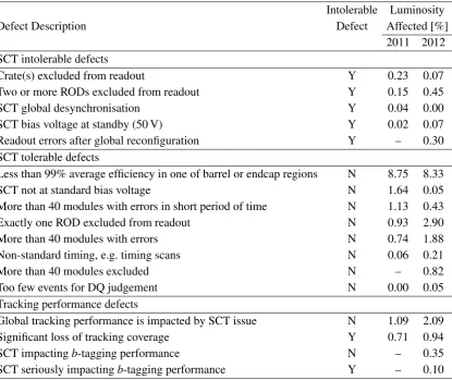
tracking coverage in a region of the detector. The exclusion of RODs or crates affects a limited but significant region of the detector. Other intolerable defects affect the whole detector. The global reconfiguration of all readout chips occasionally causes data errors for a short period; the SCT can become desynchronised from the rest of ATLAS; occasionally data are recorded with the modules at standby voltage (50 V).

For more minor issues, or when the excluded modules have less of an impact on tracking coverage, a tolerable defect is set. These defects are shown in the central part of table 4. One excluded ROD is included in this category. A single excluded ROD in the endcap (the most usual case) has little impact on tracking because it generally serves modules on one disk only. A ROD in the barrel serves modules in all layers in an azimuthal sector, and thus may affect tracking performance; this is assessed as part of the global tracking performance checks. Other tolerable defects include more than 40 modules excluded from the readout or giving readout errors, which indicate detector problems but do not significantly affect tracking performance. Although noise occupancy is monitored, no defect is set for excessive noise occupancy.

In addition to SCT-specific checks, the global tracking performance of the inner detector is also evaluated, and may indicate problems which arise from the SCT but which are not flagged with SCT defects, or which are flagged as tolerable by the SCT but are intolerable when the whole inner detector is considered. This corresponds to situations where the pixel detector or TRT have a simultaneous minor problem in a similar angular region. The fraction of data affected by issues de-termined from global tracking performance is given in the lower part of table4. There is significant overlap between the SCT defects and the tracking performance defects.

The total fraction of data flagged as bad for physics in 2011 (2012) by SCT-specific checks was 0.44% (0.89%). A further 0.33% (0.56%) of data in 2011 (2012) was flagged as bad for physics by tracking performance checks but not by the SCT alone. The higher fraction in 2012 mainly resulted from RODs disabled due to high occupancy and trigger rates, as discussed in section3.4.

5.4 Prompt calibration loop

Reconstruction of ATLAS data proceeds in two stages. First a fraction of the data from each run is reconstructed immediately, to allow detailed data quality and detector performance checks. This is followed by bulk reconstruction some 24–48 hours after the end of the run. This delay allows time for updated detector calibrations to be obtained. For the SCT no offline calibrations are performed during this prompt calibration loop, but the period is used to obtain conditions data. In particular, strips that have become noisy since the last online calibration period are found and excluded from the subsequent bulk reconstruction. Other conditions data, such as dead strips or chips, are obtained for monitoring the SCT performance.

The search for noisy strips uses a special data stream triggered on empty bunch crossings, so that no collision hits should be present. Events are written to this stream at a rate of 2–10 Hz, giving sufficient data to determine noisy strips run by run for all but the shortest runs. Processing is per-formed automatically on the CERN Tier0 computers and the results are uploaded to the conditions database after a check by the shifter.

2014 JINST 9 P08009

Table 4.The data quality defects recorded for 2011 and 2012, and percentage of the luminosity affected. The

data assigned intolerable defects (marked ‘Y’ in the table) are not included in physics analyses. Empty en-tries indicate that the defect was not defined for that year. Multiple defect flags may be set for the same data.

Intolerable Luminosity

Defect Description Defect Affected [%]

2011 2012 SCT intolerable defects

Crate(s) excluded from readout Y 0.23 0.07

Two or more RODs excluded from readout Y 0.15 0.45

SCT global desynchronisation Y 0.04 0.00

SCT bias voltage at standby (50 V) Y 0.02 0.07

Readout errors after global reconfiguration Y – 0.30 SCT tolerable defects

Less than 99% average efficiency in one of barrel or endcap regions N 8.75 8.33

SCT not at standard bias voltage N 1.64 0.05

More than 40 modules with errors in short period of time N 1.13 0.43

Exactly one ROD excluded from readout N 0.93 2.90

More than 40 modules with errors N 0.74 1.88

Non-standard timing, e.g. timing scans N 0.06 0.21

More than 40 modules excluded N – 0.82

Too few events for DQ judgement N 0.00 0.05

Tracking performance defects

Global tracking performance is impacted by SCT issue N 1.09 2.09

Significant loss of tracking coverage Y 0.71 0.94

SCT impactingb-tagging performance N – 0.35

SCT seriously impactingb-tagging performance Y – 0.10

a few thousand during 2012, as shown in figure10. Significant fluctuations are observed from run to run. These arise from two sources: single-event upsets causing whole chips to become noisy and the abnormal leakage-current increases observed in some endcap modules (see section7). Both of these effects depend on the instantaneous luminosity, and thus vary from run to run. The maximum number of noisy strips, observed in a few runs, corresponds to<0.25% of the total number of strips in the detector.

6 Performance

6.1 Detector occupancy

2014 JINST 9 P08009

Number of strips

1 10 2 10 3 10 4 10 Fraction [%] -4 10 -3 10 -2 10 -1 10 ATLAS SCT

Noisy strips identified in the prompt calibration loop

Figure 10. Number of noisy strips (also shown as the fraction of all strips on the right-hand axis) found in

the prompt calibration loop for physics runs with greater than one hour of stable beams during 2010–2013. Noisy strips identified in online calibration data are excluded from the total.

Number of interactions per bunch crossing

10 20 30 40 50 60 70 80

Occupancy 0 0.005 0.01 0.015 0.02 0.025 Barrel 3 Barrel 4 Barrel 5 Barrel 6 ATLAS SCT Barrel (a)

Number of interactions per bunch crossing

10 20 30 40 50 60 70 80

Occupancy 0 0.002 0.004 0.006 0.008 0.01 0.012 0.014 0.016 0.018 0.02 Outer Middle Inner ATLAS

SCT Endcap Disk 3

(b)

Figure 11.Mean occupancy of (a) each barrel and (b) inner, middle and outer modules of endcap disk 3 as

a function of the number of interactions per bunch crossing in minimum-biasppdata. Values for less than 40 interactions per bunch crossing are from collisions at√s= 7 TeV, those for higher values from collisions at√s= 8 TeV, which have an occupancy larger by a factor of about 1.03 for the same number of interactions per bunch crossing.

mean strip occupancy was expected to be less than 1%. In 2012 with an LHC bunch-spacing of 50 ns the design goals for pile-up were exceeded with no significant loss of tracking efficiency.

2014 JINST 9 P08009

0 20 40 60 80 100 120

Maximum sustainable rate [kHz]

0 100 200 300 400 500 600

ATLAS SCT

= 8 TeV s

(a)

µ

0 20 40 60 80 100 120

Maximum sustainable rate [kHz]

0 100 200 300 400 500 600

ATLAS SCT

= 8 TeV s

(b)

Figure 12.Maximum sustainable level-1 trigger rate for the transfer of data from (a) front-end chip to ROD

and (b) ROD to ATLAS DAQ chain, as a function of the mean number of interactions per bunch crossing,

µ. Values are calculated from measured event sizes in ppinteractions at √s= 8 TeV assuming 90% of the available data-link bandwidth is used. Each link is shown as a separate curve. Increasing numbers of superimposed curves are indicated by changes of colour from blue through green and yellow to red. The dashed lines indicate the typical 2012 trigger rate of 70 kHz.

or the prompt calibration loop were removed. The data were recorded using a minimum-bias trigger in special high pile-up runs, where average numbers of interactions per bunch crossing greater than the 35 routinely seen in physics runs could be achieved, and events were required to have at least one reconstructed primary vertex. Values for less than 40 interactions per bunch crossing are from collisions at√s = 7 TeV, those for higher values from collisions at√s = 8 TeV. The occupancy at 8 TeV is expected to be a factor of about 1.03 larger than at 7 TeV for the same number of interactions per bunch crossing. Allowing for this, good linearity is observed up to 70 interactions per crossing, where the average occupancy is less than 2% in the innermost barrel and∼1.5% in the middle modules of the central disks (the middle modules have the largest pseudorapidity coverage and hence largest occupancy in the endcaps).

2014 JINST 9 P08009

the slowest data links are still adequate up to a pile-up,µ, of 120, while the S-links impose a limit ofµ <62 at the typical 2012 trigger rate of 70 kHz.

Significant increases in trigger rate and pile-up are anticipated with the increase in instanta-neous luminosities foreseen at the LHC beyond 2015 at√s= 14 TeV. The increase in multiplicity and trigger rate will impose a reduced limit on µ of∼87 and∼33 at 100 kHz for the data links and S-links respectively, if there are no changes made to the existing DAQ. The limit from the data links arises from components mounted on the detector, and therefore cannot be improved. The limit from the S-links will be improved by increasing the number of RODs, BOCs and S-links from 90 to 128; the load per S-link will therefore be reduced and balanced in a more equal way. In addition, edge-mode readout (01X, see section2.2)) will be deployed to minimise the effect of hits from one bunch crossing appearing in another, and an improved data-compression algorithm will be deployed in the ROD. As a result of these changes, the slowest S-link will be able to sustain a level-1 trigger rate of 100 kHz atµ = 87, which matches the hard limit from the front-end data links. This corresponds to a luminosity of 3.2×1034cm−2s−1 with 25 ns bunch spacing and 2808 bunches per beam.

6.2 Noise

One of the crucial conditions for maintaining high tracking efficiency is to keep the read-out thresh-olds as low as possible. This is only possible when the input noise level is kept low. There are two ways of measuring the input equivalent noise charge (ENC, in units of number of electrons) in dedicated calibration runs:

1. Response-curve noise: in three-point gain-calibration runs, a threshold scan is performed with a known charge injected into each channel, as described in section3.2. The Gaussian spread of the output noise value at the injection charge of 2 fC (chosen because this value is well clear of non-linearities which can appear below 1 fC) is obtained by fitting the threshold curve. The ENC is calculated by dividing the output noise by the calibration gain of the front-end amplifier.

2. Noise Occupancy (NO):in the noise-occupancy calibration runs, a threshold scan with no charge injection is performed to obtain the occupancy as a function of threshold charge. The ENC is estimated from a linear fit to the dependence on threshold charge of the logarithm of noise occupancy.

The former value reflects the width of the Gaussian-like noise distribution around±1σ while the latter is a measure of the noise tail at around +4σ, being sensitive to external sources such as common-mode noise. Whenever the corresponding calibration runs are performed, the mean values of the response-curve ENC or NO at 1 fC for each chip are saved for later analyses. These two noise estimates correlate fairly well chip-by-chip, but ENC values deduced from noise occupancies are sytematically smaller by about 5% [42]. Below, unless specified, ‘noise’ refers to the ENC value from the response-curve width, and is measured for modules with bias voltage at the normal operating value of 150 V.

2014 JINST 9 P08009

only modules with<111>sensors are plotted; barrel 6, which has a higher temperature and thus higher noise, is shown separately from the other three barrels. For the endcaps, chips reading out Hamamatsu and CiS sensors are shown separately. Clusters around 1000 electrons in figure13a reflect the shorter strip lengths of endcap inner and middle-short sensors. Noise occupancies of endcap inner and middle-short modules are not shown due to large errors on the low occupancy values. Almost all chips satisfy the SCT requirement of less than 5×10−4in noise occupancy for both periods.

(a) (b)

Figure 13. Distributions of chip-averaged (a) ENC from response-curve tests and (b) noise occupancy at

1 fC from calibration runs as of October 2010 (top) and December 2012 (bottom) for different types of module.

2014 JINST 9 P08009

Table 5. Mean values of ENC from response-curve tests and noise occupancies (NO) at 1 fC, obtained in

calibration runs in October 2010 and December 2012. Values are shown for each module type, separated according to sensor manufacturer or crystal orientation. The mean temperatures measured by thermistors mounted on the hybrid circuits of each module were around 2.5◦C for barrels 3–5, 10◦C for barrel 6 and 8◦C for the endcaps, and varied by less than one degree between October 2010 and December 2012. The last column shows ratios of ENC values measured in 2012 to those measured in 2010 corrected for the small temperature differences. Uncertainties in the ratios are less than 1%.

Module Type Manufacturer October 2010 December 2012 <ENC>2012

<ENC>2010

<ENC> <NO> <ENC> <NO>

Barrels 3–5 111 Hamamatsu 1470 7.5·10

−6 _{1468 9.0·10}−6 _0.997

100 Hamamatsu 1362 1.6·10−6 1394 3.1·10−6 1.021

Barrel 6 111 Hamamatsu 1521 1.3·10

−5 _{1524 1.5·10}−5 _1.001

100 Hamamatsu 1396 2.4·10−6 1436 4.8·10−6 1.028

EC inner 111 Hamamatsu 1069 — 1129 — 1.058

111 CiS 1070 — 1136 — 1.065

EC middle 111 Hamamatsu 1472 8.0·10

−6 _{1469 2.1·10}−5 _1.000

111 CiS 1513 1.4·10−5 1662 9.5·10−5 1.102

middle short 111 CiS 895 — 1004 — 1.124

EC outer 111 Hamamatsu 1568 1.6·10−5 1553 3.9·10−5 0.993

The evolution of the response-curve noise as well as the front-end gains obtained in calibration runs from 2010 to 2012 is shown in figure14; modules are divided into ten different groups as in table5. All the gains are rather stable except the gradual and universal change of a few percent in mid 2011 and early 2012, the reason for which is not clear.

As can be seen in figure 14, the noise decreased by about 7% in late 2010 when the fluence level at the modules was around 1010cm−2, a dose level of a few Gy. The noise drop varied strongly with the strip location as shown by the chip-number dependence in figure15for barrel 5 as an example. It occurred systematically in all modules except those with <100>sensors. In addition, the decrease occurred first in barrel 3 and later in barrel 6 indicating fluence-dependent effects. Similar noise decreases were observed in the endcap modules but they strongly depended on the module side. Disconnected strip channels showed no decrease. In 2011 and 2012, no such noise decrease was observed, rather the noise returned to the original value and the chip-number dependence disappeared as shown by the 2011 points in figure 15. A beam test at the CERN-PS with a low rate reproduced qualitatively such a trend at a similar dose level. This unexpected phenomenon is probably caused by charge accumulated on the sensor surface leading to effective capacitance changes.

6.3 Alignment stability

While the alignment is determined using tracks (as described in section4.2), the FSI system is used to confirm the observation of movement in the SCT.