Essays in empirical finance

(1)

University of Warwick institutional repository: http://go.warwick.ac.uk/wrap

A Thesis Submitted for the Degree of PhD at the University of Warwick

http://go.warwick.ac.uk/wrap/78174

This thesis is made available online and is protected by original copyright. Please scroll down to view the document itself.

(2)

Essays in Empirical Finance

By

Qi Xu

Warwick Business School

University of Warwick

January 2016

(3)

List of Tables

2.1 Descriptive Statistics . . . 36

2.2 In-Sample Volatility Forecasting Results . . . 37

2.3 Out-of-Sample Volatility Forecasting Results . . . 39

2.4 Out-of-Sample Portfolio Performance: Daily Rebalancing . . . . 40

2.5 In-Sample Volatility Forecasting: Average RV . . . 41

2.6 Out-of-Sample Statistical and Economic Performances: Average RV . . . 42

2.7 Out-of-Sample Portfolio Allocation with Transaction Costs . . . 43

2.8 Contemporaneous Regressions of Realized Jumps . . . 44

2.9 Realized Moments Forecasting . . . 45

2.9 Realized Moments Forecasting . . . 46

2.10 Out-of-Sample Portfolio Performance: Alternative Realized Mo-ments . . . 47

2.11 Simulation Results: Size . . . 53

2.12 Simulation Results: Size Corrected Power with Varying Intensity 54 2.13 Simulation Results: Size Corrected Power with Varying Size . . 55

2.14 In-Sample Volatility Forecasting Results . . . 59

2.15 Out-of-Sample Statistical and Economic Performances: Good and Bad Jumps . . . 60

2.16 Out-of-Sample Volatility Forecasting HAR-RV-CJ: Sub Samples 61 2.17 Out-of-Sample Volatility Timing: Sub-Samples . . . 62

3.1 List of 30 Assets . . . 107

3.2 Summary Statistics of Realized Measures . . . 108

3.3 One Day Ahead In-Sample Volatility Forecasting: SPY . . . 109

3.4 One Day Ahead In-Sample Volatility Forecasting: 30 Assets . . 110

3.5 One Day Ahead Out-of-Sample Volatility Forecasting: 30 Assets 111

3.6 Out-of-Sample Portfolio Performances Using Realized Volatility 112

(7)

3.7 Out-of-Sample Portfolio Performances Using Realized Volatility Components . . . 113

3.8 Out-of-Sample Portfolio Performances Using Realized Higher

Mo-ments . . . 114

3.9 Alternative Benchmarks and Correlation Structures . . . 115

3.10 Out-of-Sample Portfolio Performances Using Realized Volatility under MMS . . . 116 3.11 Out-of-Sample Portfolio Performances Using Realized Volatility

Components under MMS . . . 117 3.12 Out-of-Sample Portfolio Performances Using Realized Higher

Mo-ments under MMS . . . 118 3.13 Out-of-Sample Portfolio Performances Using Realized Volatility

Controlling for Transaction Costs . . . 119 3.14 Out-of-Sample Portfolio Performances Using Realized Volatility

Components Controlling for Transaction Costs . . . 120

3.15 Out-of-Sample Portfolio Performances Using Realized Higher Mo-ments Controlling for Transaction Costs . . . 121

4.1 Descriptive Statistics: Volatility Factors . . . 162

4.2 Descriptive Statistics: Currency Portfolios . . . 163

4.3 Currency Asset Pricing with Volatility Components: Factor Prices164

4.4 Currency Asset Pricing with Volatility Components: Factor Betas 165

4.5 Currency Asset Pricing with Alternative Volatility Factors:

Fac-tor Prices . . . 166

4.6 Currency Asset Pricing with Alternative Volatility Factors:

Fac-tor Betas . . . 167

4.7 Currency Asset Pricing with Volatility: Factor Mimicking

Port-folios . . . 168

4.8 Volatility Beta Sorted Portfolios . . . 169

4.9 Currency Asset Pricing with Volatility Components: Developed

Countries . . . 170 4.10 Currency Asset Pricing with Alternative Volatility Factors:

De-veloped Countries . . . 171 4.11 Currency Asset Pricing with Volatility Components: Alternative

Samples and Individual Currencies . . . 172 4.12 Currency Asset Pricing with Alternative Volatility Factors:

(8)

4.13 Currency Asset Pricing with Jump and Diffusive Volatilities: Al-ternative Measures . . . 174 4.14 Currency Asset Pricing with Short and Long Run Volatilities:

Alternative Measures . . . 175 4.15 Currency Asset Pricing with Volatility of Volatility: Alternative

Measures . . . 176 4.16 Currency Asset Pricing with Cross-Sectional Volatility:

Alterna-tive Measures . . . 177

(9)

List of Figures

4.1 Currency Volatility and Volatility Innovations . . . 178

4.2 Cumulative Currency Portfolio Returns . . . 179

4.3 Currency Asset Pricing with Realized Volatility: Pricing Errors 180

4.4 Currency Asset Pricing with Jump and Diffusive Volatilities:

Pricing Errors . . . 181

4.5 Currency Asset Pricing with Short and Long Run Volatilities:

Pricing Errors . . . 182

4.6 Currency Asset Pricing with Volatility of Volatility: Pricing

Er-rors . . . 183

4.7 Currency Asset Pricing with Cross-Sectional Volatility: Pricing

(10)

To my parents

(11)

Acknowledgement

Firstly, I would like to thank my supervisors Mark Taylor and Ingmar Nolte for

their inspiration, encouragement, and support. Mark became my first

super-visor from the third year after my previous two supersuper-visors left Warwick. He

stimulates my research interests in foreign exchange markets and inspires me to

develop interesting and feasible research ideas through discussions. Ingmar was

my first supervisor and he remains as my second supervisor after he moved to

Lancaster. He encourages me to think the use of financial econometrics

tech-niques to address existing issues in empirical finance from the very early stage

of my PhD, which partially forms the foundation of this thesis. He also gives me

the freedom to pursue topics I am interested in while always willing to provide

suggestions and supports if needed. I was influenced by both of them to

trans-late research ideas into the first draft of paper as early as possible, which will

benefit me more for my future academic career. I also thank Paul Schneider,

who was my second supervisor before he moved to Lugano. Paul introduces

me a few interesting topics, which motivates me to generate ideas for future

research.

Moreover, I thank all members in WBS Finance group. Faculty members,

es-pecially Constantinos Antoniou, Daniele Bianchi, Xing Jin, Roman Kozhan,

(12)

use-ful advices on research, teaching, or more general issues. I also benefit from

discussing with previous Warwick faculty members Valentina Corradi and

An-thony Neuberger. I further thank all my PhD Finance colleagues for friendships

and helpful conversations.

Furthermore, I thank all who kindly provide comments on my papers. My

thanks go to Torben Andersen, Peter Christoffersen, Marcelo Fernandes, Oliver

Linton, Sandra Nolte, Mark Salmon, Stephen Taylor, and seminar and

confer-ence participants in Bristol University, Lancaster University, Warwick Business

School Finance Brownbag, Money Macro Finance Conference 2015, Financial

Management Association International 2014, National University of

Singapore-Risk Management Institute Annual Singapore-Risk Management Conference 2014,

Inter-national Association for Applied Econometrics Annual Conference 2014, Society

of Financial Econometrics-Cambridge INET conference 2014, Econometric

So-ciety European Meeting 2013, International Finance and Banking Association

Annual Conference 2013. I also thank Christian Wolf (editor of Journal of

Em-pirical Finance), an anonymous associate editor, and two anonymous referees

for constructive comments.

Last but not least, I thank my parents for understanding, patience, and

uncon-ditional love. I cannot finish this thesis smoothly without their support.

(13)

Abstract

This thesis consists of three papers in the area of empirical finance. Chapter 2 investigates the role of realized jumps detected from high frequency data in predicting future volatility from both statistical and economic perspectives. We show that separating jumps from diffusion improves volatility forecasting both in-sample and out-of-sample. Moreover, we show that these statistical improve-ments can be translated into economic value. We find a risk-averse investor can significantly improve her portfolio performance by incorporating realized jumps into a volatility timing based portfolio strategy.

Chapter 3 investigates the use of high frequency data in large dimensional portfolio allocation. We consider the use of high frequency data beyond the estimation of the realized covariance matrix. Portfolio strategies using high frequency data in measuring and forecasting univariate realized volatility can generate statistically significant and economically tangible benefits compared to low frequency strategies. Moreover, using high frequency data to separate real-ized volatility into different components and construct realreal-ized higher moments can also enhance portfolio performance. Strategies using upside and downside volatility components and using realized skewness can deliver incremental eco-nomic benefits over the strategy using total realized volatility alone.

(14)

Declaration

I declare that any material contained in this thesis has not been submitted for a

degree to any other university. Chapter 2 and Chapter 3 are collaboration works

with Ingmar Nolte (Lancaster University). Chapter 4 is a collaboration work

with Ingmar Nolte and Mark Taylor (University of Warwick). I contribute by

developing research ideas, conducting empirical analyses, and writing up. My

co-authors contribute by providing constructive comments and improving the

writing.

I also declare that one paper titled “The Economic Value of Volatility Timing

with Realized Jumps ”, which is dawn from Chapter 2, has been accepted for

publication and is forthcoming in the Journal of Empirical Finance.

(15)

Chapter 1 Introduction

Volatility is the most conventional measure of risk. To make financial

deci-sions, risk-averse investors need to accurately predict future risks and better

understand current risks. This thesis consists of three papers analysing

eco-nomic implications of using volatility measures. I focus on asset allocation and

empirical asset pricing applications in equity and foreign exchange markets

re-spectively.

Chapter 2 studies the role of realized jumps in improving portfolio allocation.

An asset price process can be decomposed into jumps (large and discrete price

movement) and the diffusion component (smooth and continuous component).

The idea to incorporate jumps in portfolio allocation contexts is not new (Liu,

Longstaff, and Pan 2003, Maheu, McCurdy, and Zhao 2012). Previous

stud-ies, however, mainly rely on parametric models to estimate jump parameters.

In those contexts, jumps are simply treated as a mathematical device to

gen-erate return non-normality (Backus, Chernov, and Martin 2011). A different

stream of literature focuses on using high frequency data and nonparametric

(16)

Shephard 2006, Andersen, Bollerslev, and Dobrev 2007). Potential economic

applications of detected jumps are, however, generally missing in the literature.

Therefore, we are interested in whether realized jumps detected from high

fre-quency data contain predictive information and whether they can contribute to

portfolio allocation.

We firstly investigate the use of realized jumps in predicting future volatility.

We identify realized jumps using high frequency data of market index and seven

different nonparametric jump tests. We find that separating jumps from the

diffusion component improves volatility forecasting performance both in-sample

and out-of-sample.

We are also interested in whether such separation is economically important.

Even though separating jumps from diffusion improves volatility forecasting

performance, an investor may only be willing to access an expensive high

fre-quency dataset and implement sophisticated nonparametric tests if the

separa-tion indeed delivers economically significant benefits. We address this issue by

conducting a mean-variance portfolio allocation exercise in which a risk-averse

investor allocates her wealth between one risky asset (market index) and one

risk free rate. If separating jumps from diffusion is economically important, we

should expect the investor to be better off using a strategy with realized jumps

compared to a benchmark strategy without such decomposition. Our empirical

evidence supports this conjecture and shows that separating jumps from

diffu-sion can improve portfolio performance.

Chapter 3 analyses the use of high frequency data in relatively large

(17)

sional portfolio allocation. A few existing studies (Fleming, Kirby, and Ostdiek

2003, Bandi, Russell, and Zhu 2008) highlight the importance of high frequency

data in improving portfolio performance. However, almost all previous studies

in this area focus on the use of high frequency data in estimating the whole

realized variance-covariance matrix. Although this practice helps to capture

asset return co-movements much faster than using low frequency data, there

are two apparent drawbacks: Firstly, assets are traded at different time stamps,

and hence asset returns are usually recorded non-synchronically when the

sam-pling frequency is high. Such non-synchronicity generates non-negligible bias

in estimating the realized covariance matrix, which will subsequently affect

portfolio performance. Previous studies introduce different methods to

miti-gate the non-synchronicity problem, however, there is no consensus on it and

these corrected methods may themselves introduce additional estimation

er-rors. Therefore, we are interested in whether we can assess the use of high

frequency data in portfolio allocation while avoiding the potential problem of

non-synchronicity. The second disadvantage is that the use of a whole realized

variance-covariance matrix almost fully overlooks the segmented but fast

grow-ing stream of the literature on alternative univariate realized measures such as

realized volatility components and higher return moments (Andersen,

Boller-slev, and Diebold 2007, Patton and Sheppard 2013, Amaya, Christoffersen,

Jacobs, and Vasquez 2011). Previous studies fail to adapt these alternative

realized risk measures to a large scale portfolio allocation framework, mainly

because the technical difficulty of using these alternative realized measures and

controlling for non-synchronicity at the same time. Hence, we are also

(18)

Initially, we investigate whether using high frequency data to estimate and

fore-cast univariate realized volatilities already provides a investor with sufficiently

large economic benefits. We combine the high frequency based conditional

volatilities with a low frequency based correlation structure to composite the

conditional covariance matrix, and then solve the portfolio problem. We show

that a risk-averse investor can significantly benefit from the strategy using high

frequency data compared to a benchmark strategy purely using low frequency

data.

Moreover, high frequency data also allow us to extract realized volatility

com-ponents and construct realized higher return moments. We study the use of

these alternative realized measures as volatility predictors to improve portfolio

allocation. We find that both realized volatility components and realized higher

moment strategies can also outperform the low frequency benchmark strategy.

Strategies using upside and downside realized volatility components and

real-ized skewness can further generate incremental improvements compared to the

strategy using total realized volatility only.

Chapter 4 investigates the pricing of volatility risk in currency markets. Menkhoff,

Sarno, Schmeling, and Schrimpf (2012a) already document that volatility risk

is important for explaining currency carry trade returns. Two reasons motivate

us to revisit the pricing of currency volatility risk. Firstly, volatility risk is

especially important for understanding the risk return profile in currency

mar-kets. In equity markets, volatility risk is complementary to the equity market

factor. In currency markets, due to the lack of a consensus global currency

market factor, volatility risk is of first order importance. Previous studies on

(19)

currency volatility risk mainly rely on a simplified proxy for volatility.

There-fore, we aim to provide new insights on the pricing of volatility risk by

bet-ter understanding the volatility process. Secondly, although volatility risk is

priced in carry trade returns, previous studies (Burnside, Eichenbaum, and

Eichenbaum 2011, Menkhoff, Sarno, Schmeling, and Schrimpf 2012b) also

ad-mit that volatility risk can hardly explain currency momentum returns or the

joint cross-section of carry trade and momentum returns. We are interested in

whether we can obtain new results with our volatility factors.

Firstly, we investigate whether pricing volatility risk can be explained by

pric-ing some of its components. We decompose volatility into jump and diffusion

components and into short and long run components. We find that the

explana-tory power of volatility risk in carry trade returns is almost exclusively coming

from the diffusion component. However, neither total volatility nor the diffusive

volatility is able to explain the joint cross-section of carry trade and momentum

portfolios. Nevertheless, the jump component, which is less important for carry

trade returns, contains unique pricing ability for the joint cross-section of carry

trade and momentum portfolios. We also suggest that both short and long run

volatility components are priced in carry trade portfolios. The short run

com-ponent is slightly stronger than the long run comcom-ponent. However, neither of

them can explain the joint cross-section. Therefore our findings support that

the pricing ability of volatility risk is concentrated in some of its components.

Secondly, if the pricing of volatility risk is rationalized by a hedging argument

from the Intertemporal Capital Asset Pricing Model (ICAPM), then intuitively

(20)

in currency returns. We construct two alternative volatility factors: volatility

of volatility and cross-sectional volatility, and find that they are also priced in

carry trade returns. Moreover, we suggest that these alternative volatility

fac-tors contain unique explanatory powers for different test asset returns. Similar

to jump volatility, volatility of volatility can also explain the joint cross-section,

indicating the importance of the tail component of volatility. Cross-sectional

volatility can explain carry trade portfolio returns when we controll for

conven-tional volatility risk, and it also outperforms other measures in pricing

individ-ual currency returns. Our findings suggest that alternative volatility factors are

also priced in currency returns and they are not subsumed by the conventional

volatility risk.

To summarize, all three chapters present novel empirical evidence on the use of

different volatility measures in important economic applications and contribute

by bridging important literature gaps overlooked by previous studies.

(21)

Chapter 2 The Economic Value of Volatility

Timing with Realized Jumps

2.1 Introduction

The importance of jumps in asset pricing, option pricing, and risk

manage-ment is widely recognized (Ait-Sahalia 2004). Although, resorting on jumps

as a modeling device is not new, realized jumps were generally overlooked

un-til recently. In this paper, we comprehensively investigate the role of realized

jumps detected from high frequency data for the prediction of future volatility.

Different from previous studies with similar focus, we not only conduct an

ex-tensive statistical evaluation of volatility forecasting using all major jump tests,

but also provide new economic insights in the form of whether a risk-averse

investor can significantly benefit from considering realized jumps in volatility

timing based portfolio allocation strategies.

The literature on this topic can be broadly categorized into two streams: The

(22)

stochastic-volatility with jumps (SVJ) models in continuous time (Eraker,

Jo-hannes, and Polson 2003, Eraker 2004, Chernov, Ronald Gallant, Ghysels, and

Tauchen 2003) and GARCH-J models in discrete time (Maheu and McCurdy

2004, Duan, Ritchken, and Sun 2006, Christoffersen, Jacobs, and Ornthanalai

2012). These parametric models are widely used in portfolio choice, option

pricing, and risk management applications and the jumps introduced in models

are ex ante in nature. As Backus, Chernov, and Martin (2011) admit: “A jump

component, in this context, is simply a mathematical device that produces

non-normal distributions.”

The second stream of the literature considers nonparametric approaches.

Re-cently, many nonparametric jump tests (Barndorff-Nielsen and Shephard 2006,

Andersen, Bollerslev, and Dobrev 2007, Ait-Sahalia and Jacod 2009) use high

frequency data to estimate ex post realized jumps. This stream of the literature

primarily focuses on issues such as why asset prices jump (e.g. macroeconomic

new announcements) or how often asset prices jump (e.g. less than one per

day). However, only a very few studies consider economic applications of

real-ized jumps. We therefore aim to fill this gap between two related but different

streams of literature by considering economic applications of realized jumps.

We focus on two research questions: Firstly, we are interested in whether

re-alized jumps can forecast future volatility. We apply seven main stream

non-parametric jump tests to identify realized jumps, decompose realized variance

into jump and diffusion components, and then adapt them into a forecasting

framework. Our findings suggest that realized jumps do contain predictive

in-formation for future volatility for the majority of jump tests both in-sample and

(23)

out-of-sample. We find that jump models in general generate higher adjusted

R2_{s and lower Mean Squared Errors (MSE) compared to the benchmark model,}

which does not separate jumps from diffusion. Results hold true across the

ma-jority of jump specifications, and different forecasting horizons. Existing studies

investigate similar issues. However, they mainly rely on one particular jump test

and their results are mixed. For example, Andersen, Bollerslev, and Diebold

(2007) find a negative (but insignificant) relationship between jumps and one

period ahead volatility. Corsi, Pirino, and Reno (2010) on the contrary show

statistically significant evidence to support a positive relationship if a modified

jump test is applied. By using all major jump tests, our results contribute to

the debate whether in general realized jumps help to forecast volatility.

Incorporating realized jumps into volatility forecasting require accessing

intra-day high frequency data and applying sophisticated nonparametric jump tests.

Therefore, a natural question arises whether it is worth to estimate and use

re-alized jumps. Even though separating jumps from diffusion improves volatility

forecasting, it is interesting to know whether the improvement is large, and more

importantly whether the improvement is economically valuable. Therefore, our

second research question explicitly asks whether the potential statistical

fore-casting improvement obtained by separating jumps from diffusion can be

trans-lated into tangible economic benefits for a risk-averse investor. We construct

a mean-variance portfolio strategy based on the predicted volatility obtained

from the previous step. Our findings suggest that the statistical improvements

are also economically significant. Under different risk aversion levels and jump

specifications, jump strategies can in general generate positive and statistically

(24)

papers also consider the role of jumps in asset allocations. For example, Liu,

Longstaff, and Pan (2003) provide an analytical solution to the optimal

port-folio choice problem when event risk or jumps are considered. They find that

jumps play an important role in determining the optimal portfolio choice. Two

recent studies by Chen, Hyde, and Poon (2010) and Maheu, McCurdy, and Zhao

(2012) are also close to us in considering jumps in asset allocation. However, we

differ from those studies on a few aspects. Firstly, our nonparametric framework

enables us to exploit the information embedded in jump variations in a model

free fashion while previous papers rely on a parametric specification. Secondly,

we use high frequency data to separate the jumps and the diffusion component

precisely, while they mainly rely on daily data to obtain relatively noisy proxies

for jumps (i.e. large extraordinary movement or middle size jumps etc). The

high frequency data we use also allows us to access intraday information, which

is overlooked by previous studies.

We then conduct comprehensive robustness checks, and find that further

con-trolling for market microstructure effects and transaction costs does not change

our main results. We also investigate the predictive ability of realized jumps on

alternative realized moments. We find that realized jumps can predict realized

volatility and its signed components, but can hardly predict realized higher

mo-ments. We further show that a mean-variance portfolio strategy based on

pre-dicting positive and negative conditional volatilities separately can outperform

the benchmark strategy based on predicting total volatility, and incorporating

realized jumps can additionally improve economic benefits.

A few other studies are also related to ours. Firstly, our paper can be viewed as

(25)

a natural extension of the stream of literature considering the economic value

of volatility timing. Previous studies (Fleming, Kirby, and Ostdiek 2003, Bandi

and Russell 2006, Bandi, Russell, and Zhu 2008, Liu 2009) already document

that volatility timing performance can be improved by using high frequency

data, optimal sampling, and optimal rebalancing frequencies. We extend the

above studies by considering realized jumps. Secondly, our paper is also related

to other uses of realized jumps or applications of jump tests. For example,

Dumitru and Urga (2012) and Theodosiou and Zikes (2011) conduct

compre-hensive simulation studies to compare size and power of jump tests. Tauchen

and Zhou (2011) and Jiang and Yao (2013) use detected realized jumps to

pre-dict bond risk premia and the cross-section of stock returns respectively. We

distinguish ours from previous studies by focusing on the role of realized jumps

in volatility timing.

The rest of the paper is structured as follows: Section 2.2 discusses the

theoret-ical setup and the jump tests. Section 2.3 describes the data and methodology.

Section 2.4 discusses empirical findings from both statistical and economic

per-spectives. Section 2.5 conducts comprehensive robustness checks. Section 2.6

(26)

2.2 Jumps in Asset Prices

2.2.1 Theoretical Setup

Letptdenote the logarithmic price which follows a jump diffusion process given

by

dpt =µtdt+σtdWt+dJt (2.1)

where µt, σt, and dWt are drift, diffusion parameter, and standard brownian

motion respectively. Jt is a jump process, and Jt = PjN=1t ctj, where ctj is the

jump size and Nt a counting process. For simplicity, we only consider finite

activity jumps and we assume that the jump and the diffusion components are

independent. Let

rj,t =p₍_t₋₁₎_h₊hj

M −p(t−1)h+ h(j−1)

M , j = 1, . . . , M,

whereh is the length of the intraday sampling interval andM is the number of

intraday returns during the day. Then the realized variance can be written as

the sum of the squared intraday returns

RVt=RVt,M = M

X

j=1

r_j,t2

Given the price dynamics of the jump diffusion process, the realized variance

as an approximation to the price’s quadratic variance can be further written as

follows

lim

M→∞RVt,M =

t

Z

t−1

σ_s2ds+

Nt X

j=1

c2_j (2.2)

(27)

Here R_tt₋₁σ2

sds is the integrated variance (IVt), and PN_j₌₁t c2j is the quadratic

variation of the jump part (JVt) over the period from t−1 to t (often a day).

Jump tests are therefore designed to estimate JVt using high frequency data.

2.2.2 Jump Tests

We consider the use of seven major jump tests developed in the literature,

in-cluding Barndorff-Nielsen and Shephard (2006) (BNS), Ait-Sahalia and Jacod

(2009)(AJ), Jiang and Oomen (2008)(JO), Andersen, Dobrev, and Schaumburg

(2012) (Med, Min), Corsi, Pirino, and Reno (2010)(CPR), and Podolskij and

Ziggel (2010) (PZ). In this part, we only describe the BNS jump test in detail.

Specifications of all other six tests are described in Appendix 1. Andersen,

Bollerslev, and Dobrev (2007) and Lee and Mykland (2008) are two other

im-portant tests that are however not studied in this paper.1

Barndorff-Nielsen and Shephard (2006) developed a bipower based jump

esti-mator. The idea is using the calculated realized bipower variation to proxy the

integrated variance. Since jumps are rare and are unlikely to occur for two

con-secutive intraday returns, when intervals are small enough, the realized bipower

variation will converge in probability to the integrated variance. The difference

between realized variance and realized bipower variation is then an estimator

1_{The reason is that both of them are intraday jump tests that average daily bipower variation to}

(28)

of the jump variation. The realized bipower statistic is defined as

BVt,M =

µ−₁2M

M ₋1

M

X

j=2

|rtj−1||rtj|,

lim

M→∞BVt,M −→IV =

t

Z

0

σ_s2ds.

Following Huang and Tauchen (2005), the standardizedBVt,M/RVt,M ratio

con-verges to a standard normal distribution and the test statistic is given by

Jt,M =

1₋ BVt,M

RVt,M q

[(2_π)2₊_π₋_5]1

Mmax(1, T Qt,M

BV2

t,M)

−→N(0,1), (2.3)

where T Qt refers to the tripower quarticity given by

T Qt,M =Mµ−₄_/3₃

M

M₋2

n

X

j=3

|rj−2|4/3|rj−1|4/3|rj|4/3,

where µp =E(|U|)p =π−1/22p/2Γ(p+1₂ ).

The jump variation can then be obtained as

JVt= (RVt−BVt)I_[_J_t,M_≥_φ−1

α ], (2.4)

where the φ−1

α is the α quantile of the normal distribution.

(29)

2.3 Data and Methodology

2.3.1 Realized Jumps and Volatility Forecasting

We first investigate the role of realized jumps in volatility forecasting. There

are many approaches to forecast volatility using high frequency data. We use

the Heterogeneous Autoregressive (HAR) model of Corsi (2009) because it can

be implemented easily and it can capture the long memory property of volatility

processes in a straightforward way. Our benchmark model considers the use of

daily, weekly, and monthly lagged realized variances to forecast one step ahead

realized variance. The HAR-RV specification is as follows:

RVt,t+h−1 =β0+βRV DRVt−1+βRV WRVt−5,t−1+βRV MRVt−22,t−1+ǫt,t+h−1. (2.5)

To assess the role of jumps, we consider the following HAR-RV-CJ specification:

RVt,t+h−1 =β0+βIV DIVt−1+βIV WIVt−5,t−1+βIV MIVt−22,t−1+βJV DJVt−1+ǫt,t+h−1

(2.6)

where RVt,t+h =h−1[RVt+RVt+1...+RVt+h−1] is the averaged h-periods

real-ized variance. IVt−1, IVt−5,t−1, IVt−22,t−1 are jump robust integrated variation

estimators over a lagged daily, weekly, and monthly horizon, JVt−1 is the daily

lagged jump variation detected using the jump tests introduced before.

2.3.2 Realized Jumps and Volatility Timing Based

Port-folio Strategy

We then conduct our economic evaluations by constructing volatility timing

(30)

mean-variance preferences, who allocates her wealth into one risky asset (a

market index ETF) and one risk-free asset. Our one risky asset specification

is similar to Marquering and Verbeek (2004). The economic intuition for this

strategy is simple. Given the expected return, when the volatility level is high,

the investor allocates more wealth into the risk-free asset, and when the

volatil-ity level is low, the investor allocates more wealth into the risky asset. If

separating jumps from diffusion components lead to more accurate prediction

of future volatility, then we should expect the investor to improve her portfolio

performance by actively rebalancing the portfolio based on the signal of the

predicted volatility.

Although more sophisticated utility functions can be used, we stick to

mean-variance preferences because we are primarily interested in whether statistical

improvements in volatility forecasting by separating jumps from diffusion can

be translated into economic values. To concentrate on the impact of jumps,

we consider only one market index as the risky asset. We choose this setting

to avoid dealing with jump tests in multivariate settings and controlling for

non-synchronicity of different assets, while we still maintain the generality of

our empirical results. We also assume that the investor is myopic. Namely, the

investor dynamically rebalances her portfolio period by period, and she does

not consider the intertemporal hedging demand in the portfolio selection. We

make this assumption both for simplicity to directly translate our volatility

fore-casting results into portfolio performance and for consistency with the existing

volatility timing literature.

(31)

Hence, the investor solves the following optimization problem:

Max

wt

U[Et(rp,t+1), V art(rp,t+1)],

where Et(rp,t+1) is the conditional expected portfolio return and V art(rp,t+1)

is the conditional variance of the portfolio return. The portfolio return is

Et(rp,t+1) = rf,t+1 +wt(Et(rm,t+1) −rf,t+1), where wt is the portfolio weight

of the risky asset, Et(rm,t+1) is the conditional expected return of the risky

as-set andrf,t+1 is the return for the risk free asset, which we know ex ante.

The mean-variance utility function is given by

U[Et(rp,t+1), V art(rp,t+1)] = Et(rp,t+1)−

γ

2V art(rp,t+1),

with γ the risk-aversion parameter. Hence, the optimal portfolio weight is

given by

wt=

Et(rm,t+1)−rf,t+1

γV art(rm,t+1)

. (2.7)

We set the expected return for the risky asset equal to the in-sample mean 2_,

as over a short horizon, expected return changes are negligible and we are only

interested in the volatility timing effect of realized jumps.

Fleming, Kirby, and Ostdiek (2003) show that using a dynamic volatility timing

strategy relying solely on realized volatilities can outperform both static

strate-gies and dynamic volatility timing stratestrate-gies using lagged daily volatilities only.

Therefore the question whether realized jumps are economically valuable can be

translated into whether our jump augmented volatility timing strategy

(32)

RV-CJ) can outperform the benchmark strategy (HAR-RV) which does not

separate jumps from the diffusion component.

To implement the above strategy, we conduct two further adjustments. Firstly,

we impose a short selling constraint. Following Marquering and Verbeek (2004),

we restrict the negative portfolio weights to zero and the greater than one

port-folio weights to one. Secondly, we also match the high frequency trading period

(6.5 hour) to daily frequency (24 hour). Therefore, rather than directly

plug-ging in the predicted realized variance, we adjust the predicted realized variance

with a bias-correction factor. We follow existing studies (Fleming, Kirby, and

Ostdiek 2003, Bandi and Russell 2006) and construct the bias-correction factor

as follows:

BCF = 1/n

Pn t=1rt2

1/nPn_t₌₁RVt

, (2.8)

where RVt is the daily realized variance for 6.5 trading hours and rt is the

daily return for 24 hours. We construct the bias-correction factor using all data

from the in-sample period. The conditional variance is estimated by predicted

realized variance scaled by the bias correction factor, namely V art(rm,t+1) =

BCF_·RVdt+1, whereRVdt+1 is the predicted realized variance obtained from the

volatility forecasting part. We can then plug in the conditional variance into

the optimal portfolio weight function to estimate the optimal portfolio weight.

2.3.3 Performance Evaluations

Following the volatility timing literature, we focus on the utility based

perfor-mance evaluation measure to assess whether investors can benefit from including

realized jumps into their information set. We follow Fleming, Kirby, and

Ost-diek (2003) and Marquering and Verbeek (2004) and rely on averaged realized

(33)

utility to compare jump strategies to the benchmark strategy.

The sample averaged realized utility for portfolio strategy pis given by

¯

U(Rp) =

1

T

T−1

X

t=0

[rp,t+1−

γ

2V art(rp,t+1)]. (2.9)

Given the optimal portfolio weights, we can compute daily time series of ex post

portfolio returnsrp,t+1 =rf,t+1+wt(rm,t+1−rf,t+1) and variancesV art(rp,t+1) =

(rp,t+1−r¯p)2, and then plug that in to obtain the averaged realized utility.3

To quantify the economic benefit relative to the benchmark strategy, we use the

performance fee ∆ (in basis points), which is the fee that an investor is willing to

pay to switch from the benchmark strategy (with portfolio returnrbm,t ) to our

strategy (e.g. strategypwith portfolio returnrp,t). In our analysis, we consider

different risk aversion levels (γ = 2,6,10). The performance fee is computed as

follows:

1

T

T−1

X

t=0

[(rp,t+1−∆)−

γ

2V art(rp,t+1)] =

1

T

T−1

X

t=0

[rbm,t+1−

γ

2V art(rbm,t+1)].(2.10)

2.3.4 Statistical Significance of Economic Values

One of the major concerns of existing studies on the economic value of

re-turn/volatilty prediction is the statistical significance of the economic value

obtained. The economic value computed is just a figure and usually not large

(e.g in the unit of basis points), hence we don’t know whether the value is

signif-icantly different from zero across different strategies. Therefore different

meth-3_{Alternatively, we can estimate the portfolio variance from the variance of the risky asset (we}

can use ex post realized variance scaled with the bias correction factor) scaled by the squared weight,V ar(r ) =w2_{V ar}₍_r _{) =}_w2_BCF

(34)

ods have been used to investigate the statistical significance of economic values.

Following Engle and Colacito (2006) and Bandi, Russell, and Zhu (2008), we

address this concern by viewing the economic gains as loss differential in which

we compare one portfolio to the benchmark portfolio. The approach is in the

spirit of Diebold and Mariano (1995). The Diebold-Mariano (DM) test was

designed to examine whether the loss differential of two forecasts is statistically

significantly different from zero. The test can be used when the loss differential

series is covariance stationary. Engle and Colacito (2006) and Bandi, Russell,

and Zhu (2008) applied it to examine whether the ex post

portfolio-volatility-difference between a candidate strategy and a benchmark strategy is statistically

significantly different from zero. In our study, we investigate whether the

per-formance fees (viewed as loss differential) are significantly different from zero.

We first compute the time series of daily “spot” realized utilities and then the

time series of daily performance fees for each strategy in comparison to the

benchmark. Afterwards, we construct the DM statistics and test whether the

alternative strategies do not outperform the benchmark (null hypothesis) using

a one-sided t-test with a robust variance covariance estimator.4

2.3.5 Data Description

In our empirical analysis we use the S&P500 ETF or SPDR contract (SPY)

as the risky asset, obtained from NYSE TAQ database. The contract tracks

the S&P500 index and is very liquidly traded. Trading spans from 9:30 EST to

16:00 EST. Our sample spans from Jan 2nd 2001 to Dec 31st 2010. To start with

we compute the realized volatility estimator based on equidistant observations

4_{An alternative way to assess the statistical significance of economic gains is to use bootrapping}

methods. A recent study by McCracken and Valente (2013) provides a formal test of economic values using the bootstrapping method.

(35)

sampled at the conventional five minute frequency in order to control for

mar-ket microstructure noise. In the robustness checks section, we also report the

results of a more advanced estimator to control for market microstructure noise

– the average RV estimator of Andersen, Bollerslev, Christoffersen, and Diebold

(2011). This estimator is a sub-sample estimator that can also be constructed

easily. Starting from one minute regular spaced log-returns, we compute the

average RV as an equally-weighted average of five overlapping five minute RV

estimators. Andersen, Bollerslev, and Meddahi (2011) found that the average

RV estimator can perform as well as more complex estimators (realized kernel,

multiple time scale, pre-averaging etc) in volatility forecasting. We implement

two further adjustments: Firstly, we remove the overnight periods. Secondly,

we use linear interpolation to correct for different trading hours, especially in

December 2008 and afterwards. We also collect S&P500 ETF or SPDR contract

(SPY) daily data from CRSP in order to match intraday trading period to daily

frequency. As the risk-free asset we use the daily average of the one month US

Treasury bill series.

2.4 Empirical Findings

2.4.1 Statistical Findings

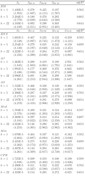
This part presents volatility forecasting results using realized jumps. Table

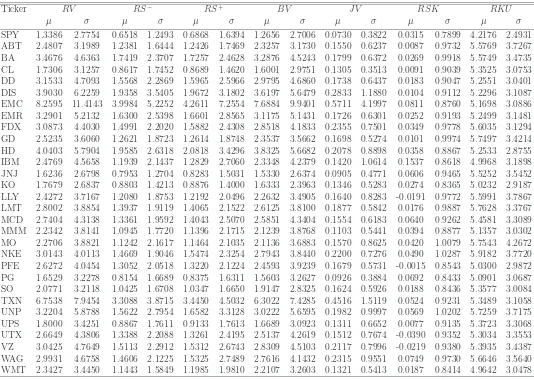
2.1 documents the descriptive statistics for the realized variance and realized

jump variations using different jump tests. Although the statistics from

differ-ent jump tests look differdiffer-ent, they all share the same features, including high

skewness and high kurtosis, supporting the asymmetric and rare event nature

(36)

models with the whole sample data from 2001 and 2010.

Table 2.2 shows in-sample volatility forecasting results for the benchmark model

and models using different jump tests. We follow Andersen, Bollerslev, and

Diebold (2007) and use the Newey-West variance covariance matrix estimator

with 5, 10 and 44 lags for daily, weekly, and monthly ahead forecasts. For the

benchmark HAR-RV model, the one day ahead forecast shows that only the

coefficient of weekly lagged realized variance is significant at the 5% level, while

for one week and one month ahead forecasts all three lagged realized variance

coefficients are significant. The adjusted R2 _{takes values of 0.562, 0.682 and}

0.644 for the different forecasting horizons. We then look at the HAR-RV-CJ

models using different jump tests. At least four points are worth mentioning.

Firstly, although at weekly and monthly horizons, coefficients for the integrated

variances are all significant as in the benchmark model, the HAR-RV-CJ results

differ from the HAR-RV model at daily horizon. The daily lagged integrated

variances now become significant, indicating that jump robust integrated

varia-tion is more important than total realized variance in daily volatility forecasting.

Secondly, the jump signs are almost all negative.5 _{Our result is consistent with}

Andersen, Bollerslev, and Diebold (2007), but is different from Corsi, Pirino,

and Reno (2010). Therefore, Corsi, Pirino, and Reno (2010)’s explanation that

larger jumps lead to higher future volatility due to an increased level of

disagree-ment may not hold in our setup. Instead, our findings are more consistent with

Andersen, Bollerslev, and Diebold (2007)’s explanation that jumps are quickly

mean reverting and hence can lead to a lower volatility rather than a higher one.

Thirdly, jump coefficients differ in terms of the significance. Jump coefficients

5_{The exception of AJ and its later relative weak statistical performance can mainly be justified}

by its finite sample properties in a simulation analysis reported in the Appendix.

(37)

are significant across all horizons for BNS, JO and PZ, significant only at daily

horizon for Med, Min, CPR, and insignificant for AJ across all horizons at the

5% level. Finally, we look at the goodness-of-fit of the models. We find that

almost all models with different jump specifications can outperform the

bench-mark HAR-RV model at all forecasting horizons. At daily level, the highest

adjusted R2 is PZ of 0.604 and the lowest is AJ of 0.562. BNS has an adjusted

R2 _{of 0.592. Compared to BNS, CPR, JO, and Med have higher adjusted} _R2_s

while Min has a lower adjusted R2_{. For weekly and monthly ahead forecasts,}

adjusted R2_{s are all close to 0.70 and 0.65 respectively. Although we observe a}

clear inverse U shape pattern of adjusted R2_{s levels across forecasting horizons}

for all models, the improvements in adjusted R2_{s compared to the benchmark}

model are diminishing from about 3% on daily horizon to about 1% on average

on weekly and monthly horizons.

Although in-sample findings document a clear improvement in volatility

fore-casting by separating jumps from diffusion, we are also interested in whether

results hold true out-of-sample. We first estimate model parameters using the

first 1000 days of the whole sample as the in-sample period, and then use the

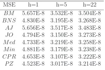
rest of the sample from 2006 to 2010 as the out-of-sample period. Table 2.3

reports our out-of-sample volatility forecasting results. We report the Mean

Squared Error (MSE) for the predicted value compared to the realized value.

Similar to the in-sample analysis, we find that all HAR-RV-CJ models using

different jump tests can outperform the benchmark HAR-RV in terms of lower

MSEs. This finding holds true for all daily, weekly, and monthly horizons.

Sim-ilar to the in-sample findings, we observe i) the largest statistical improvements

(38)

in-crease. When we compare out-of-sample findings across different jump tests, we

find that AJ has the lowest out-of-sample performance. Models using PZ, CPR,

Med, or JO outperform BNS while the model using Min underperforms BNS.

Results are consistent with in-sample findings and hold true across forecasting

horizons.

2.4.2 Out-of-Sample Economic Findings

Given the significant statistical improvement by separating jump and diffusion

components, we are now interested in whether such statistical accuracy can be

translated into economic value for a risk-averse investor. We construct

volatil-ity timing strategies as discussed above for our out-of-sample period (2006 to

2010). The largest statistical forecasting improvement was observed for a daily

horizon and given that the jump effect is quickly mean reverting we concentrate

on volatility timing with daily re-balancing. To calculate the optimal

portfo-lio weights we use the model-predicted volatility as a predictor for conditional

volatility, and then adjust it with the bias-correction factor as illustrated in

equation (2.8).

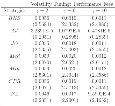
Table 2.4 reports the out-of-sample economic findings. Our main performance

measure is performance fee, interpreted as the fee that an investor is willing

to pay to switch from a benchmark strategy to a jump augmented strategy.

We consider three risk aversion levels γ = 2,6,10. We show that all jump

strategies generate positive performance fees in comparison to the benchmark

strategy, and the economic values generated depend on different jump

strate-gies and risk aversion levels. For the moderate risk aversion level of 6, we show

that highest performance fees are 20 basis points for Med and Min, followed

(39)

by 19 basis points for BNS and CPR, and 18 and 17 basis points for JO and

PZ. AJ generates positive but very small performance fee; a result that is

con-sistent with its negligible forecasting improvement in the statistical part. The

economic magnitude is also affected by the change of the risk aversion level,

ranging from 59 basis points (γ = 2) to 11 basis points (γ = 10), indicating

that the strategy seems to work better for less risk averse investors. Around

0.6% annualized performance fee looks small in magnitude, and we therefore

also assess the statistical significance of the economic value generated. We find

that except for AJ, all jump strategies generate positive and statistically

sig-nificant performance fees with DM t-statistics above 2. To summarize, we find

that the separation of jumps from diffusion components improves volatility

tim-ing strategies for almost all jump tests. The out-of-sample economic findtim-ings

are generally consistent with in-sample and out-of-sample statistical findings,

although it does not necessarily match with the ranking of the in and

out-of-sample volatility forecasting analyses. One possible explanation could be that

jumps not only affect the volatility process, but also the return process, which

is not captured by our volatility timing strategies.

2.5 Robustness Checks

In this section, we conduct comprehensive robustness checks. We focus on

three issues: Firstly, our main results are based on the RV estimator sampled

as the conventional five minutes sampling frequency. It is interesting to see

whether our results still hold true under a more stringent control of market

microstructure noise. Secondly, although we show that incorporating realized

jumps in volatility timing generates economic value, we are also interested in

(40)

costs. Thirdly, we also discuss whether realized jumps can help to predict

realized higher moments and semi-variances, and whether performances can

be improved using these in the portfolio allocation. Further extensions and

robustness checks including simulation analysis, good and bad jumps, and

sub-sample analysis can be found in the Appendix6_.

2.5.1 Market Microstructure Noises

We follow Andersen, Bollerslev, Christoffersen, and Diebold (2011) and

Ander-sen, Bollerslev, and Meddahi (2011) and construct average realized variances

and bipower variations. Table 2.5 reports the in-sample volatility forecasting

results after further controlling for market microstructure noises. Although the

jump coefficient is still negative and significant as shown in Section 2.3.2, the

adjusted R2 _{is different. For the one day ahead forecast, the adjusted} _R2 _for

the benchmark model raises from 0.562 to 0.588 when using the average RV

estimator. Similarly, the adjusted adjusted R2 _{for the HAR-RV-CJ with BNS}

raises from 0.592 to 0.628. A similar statistical improvement is also found in

the out-of-sample evaluation as shown in panel 1 of Table 2.6. Such

statisti-cal improvements by using subsample estimators also indicate potential

eco-nomic improvements. The out-of-sample portfolio allocation results are shown

in panel 2 of Table 2.6. We find that performance fees remain positive and

sta-tistically significant. Moreover, we show that economic magnitudes are larger

using the microstructure noise robust estimators compared to the conventional

five minutes estimator. A risk-averse investor is willing to pay performance fees

ranging from 62 basis points (γ = 2) to 12 basis points (γ = 10) to use a jump

6_{In our earlier version of the paper, we also show the results of an alternative parametric}

portfolio allocation strategies using realized jumps, the economic values are positive but small in magnitude and in general statistically insignificant.

(41)

strategy. Our findings suggest that the statistical and economic improvements

by separating jumps from diffusion are not likely to be driven by market

mi-crostructure noises. Instead, we show that controlling for market mimi-crostructure

noises strengthens our findings. Our results are also consistent with previous

studies (Bandi and Russell 2006, Bandi, Russell, and Zhu 2008, Liu 2009) that

controlling for microstructure noises improve portfolio performances.

2.5.2 Transaction Costs

We then analyze the impact of transaction costs on our results. Different from

existing studies comparing dynamic and static strategies (Fleming, Kirby, and

Ostdiek 2001) or comparing two dynamic strategies which are based on high

fre-quency and daily information respectively (Fleming, Kirby, and Ostdiek 2003),

our analysis compares two dynamic strategies both using high frequency

infor-mation. Therefore, we expect that the effect of transaction costs will not be

as strong as documented in the existing literature. Following Bandi, Russell,

and Zhu (2008), we define the transaction cost adjusted portfolio return in the

following way:

¯

rp,t+1 =rp,t+1−ρ(1 +rp,t+1)|∆wt+1|, (2.11)

where ¯rp,t+1 is the transaction cost adjusted portfolio return, rp,t+1 is

pre-adjusted return, ρ is the transaction cost parameter, where we choose a high

value of 0.0025, corresponding to a 2.5 cent half spread on a 10 dollar stock,

∆wt+1 is the change of the weight fromt to t+ 1, a proxy of trading turnover.

(42)

when transaction costs are taken into consideration. All specifications yield

pos-itive performance fees, implying that they can outperform the benchmark even

when transaction costs are considered. Moreover, those performance fees are

also statistically significant except for AJ. Jump strategies require

incorporat-ing recent information more quickly while the benchmark strategy is smoother,

therefore we are not surprised by the higher turnover of the jump strategies

com-pared to the benchmark strategy. Although the performance fees are slightly

lower when controlling for transaction costs, we find that our results are

gener-ally consistent with our main findings in Section 2.4.2. Moreover, the relative

performance of alternative jump specifications is also consistent with that in the

main analysis, indicating that transaction costs have similar and only marginal

effects for most of jump based volatility timing strategies.

2.5.3 Realized Jumps and Alternative Realized Moments

In practice, portfolio allocations are also subject to the impact of higher

mo-ments. Considering more general utility functions usually requires the

pre-diction of higher moments. In addition to the sophistication of incorporating

realized jumps into the portfolio allocation problem beyond mean-variance

pref-erences, we present some statistical evidence of the predictive ability of realized

jumps for alternative realized moments. We consider the use of realized jumps

for predicting realized upside and downside volatilities, skewness, and kurtosis.

We follow Barndorff-Nielsen, Kinnebrock, and Shephard (2008) and Amaya,

Christoffersen, Jacobs, and Vasquez (2011), and construct alternative realized

(43)

moments in the following way,

RV_t,M+ =

M

X

j=1

r2_j,t1rj,t>0, RV −

t,M = M

X

j=1

r_j,t2 1rj,t<0

RSKt,M =

√

MPM_j₌₁r3

j,t

(PM_j₌₁r2

i,t)3/2

, RKUt,M =

MPM_j₌₁r4

j,t

(PM_j₌₁r2

i,t)2

We first investigate the contemporaneous relationship between realized jumps

and alternative realized moments using the following regression equation:

RMt=β0+βRJRJt+ǫt, (2.12)

whereRMtis the realized moment includingRV,RV+,RV−,RSK, andRKU.

Table 2.8 presents the contemporaneous regression results. We find that

real-ized jump variation is a significant determinant of contemporaneous realreal-ized

variance, positive and negative variances, and kurtosis, explaining 18% to 80%

variation of realized moments respectively. A large jump variation is

associ-ated with a large variance, upside and downside variance, and kurtosis. Jump

variation is also negatively related to realized skewness, however the relation is

only marginally significant, and jumps can only explain about 1% variation in

skewness.

We are more interested in the predictive relationship of realized jump variation

and realized moments. Therefore we forecast realized moments using daily,

weekly, and monthly lagged realized moments in the fashion of the HAR model,

(44)

and monthly ahead forecasting horizons. The models are specified as follows:

RMt,t+h−1 =β0+βRM DRMt−1+βRM WRMt−5,t−1+βRM MRMt−22,t−1+ǫt,t+h−1.

(2.13)

To investigate the impact of jump, we then augment the model with realized

jumps.

RMt,t+h−1 =β0+βRM DRMt−1+βRM WRMt−5,t−1 +βRM MRMt−22,t−1

+βJV DJVt−1+ǫt,t+h−1.

(2.14)

Table 2.9 reports in-sample forecasting results for realized moments. The

re-sults vary across different realized moments and forecasting horizons. Firstly,

we find that realized jump helps to forecast realized variance, even though we

do not use jump robust integrated variance as we did in the main part of the

analysis. For all the forecasting horizons, we observe negative and statistically

significant jump coefficients. Moreover, the adjusted R2_{s of the models}

includ-ing jumps are higher than those of the models without jumps. This findinclud-ing

suggests that jumps do contain incremental information for predicting future

volatility and the statistical and economic improvements we documented in the

main analysis do not purely come from a better measurement of jump robust

integrated variance. We now discuss the role of jumps in predicting alternative

realized moments: We find that realized jumps have negative and statistically

significant impacts on future downside volatility for all forecasting horizons and

improvements in adjusted R2_{s range from 1% to 3%. We also find that}

real-ized jumps help to predict upside volatility at the daily horizon and generate

improvements in adjusted R2 _{of about 0}_._{2%. However, we show that realized}

jumps do not predict future realized skewness. Although realized jumps predict

(45)

realized kurtosis at daily and weekly horizons, improvements in adjusted R2_s

are almost negligible. These results, suggest that realized jumps may not

con-tain predictive information beyond second moments at least in our empirical

setups.

We then consider a simple portfolio allocation within the mean variance

frame-work to quantify the predictive ability of realized jumps on alternative realized

moments. We focus on upside and downside volatilities. Since the optimal

portfolio weight is a function of the conditional variance of the risky asset, we

can decompose it, as:

V art(rm,t+1) =V art(rm,t+1)++V art(rm,t+1)−=BCF( ˆRV +

t,t+1+ ˆRV

−

t,t+1).

(2.15)

Since jumps have different predictive abilities to forecast upside and

down-side volatilities, an investor may improve portfolio performances by forecasting

RV+_t,t₊₁ and RV−_t,t₊₁ separately and combining and scaling them by the Bias

Correction Factor to obtain the total conditional variance V art(rm,t+1), which

can then be plugged into the portfolio weights function as shown in equation

(2.7). We construct two portfolio strategies: The first strategy is based on

predicting upside and downside volatilities with their lagged values in the HAR

fashion. To improve forecasting performance, we include both upside and

(46)

component one day ahead.

RV_t,t+₊_h₋₁ =β0+βRV P DRVt+−1+βRV M DRVt−−1+βRV P WRVt+−5,t−1

+βRV M WRVt−−5,t−1+βRV P MRVt+−22,t−1+βRV M MRVt−−22,t−1+ǫt,t+h−1,

(2.16)

RV_t,t−₊_h₋₁ =β0+βRV P DRVt+−1+βRV M DRVt−−1+βRV P WRVt+−5,t−1

+βRV M WRVt−−5,t−1+βRV P MRVt+−22,t−1+βRV M MRVt−−22,t−1+ǫt,t+h−1.

(2.17)

The second strategy augments the first strategy with daily lagged realized jump

variation as additional regressor.

RV_t,t+₊_h₋₁ =β0+βRV P DRVt+−1 +βRV M DRVt−−1+βRV P WRVt+−5,t−1

+βRV M WRVt−−5,t−1+βRV P MRVt+−22,t−1+βRV M MRVt−−22,t−1

+βJV DJVt−1+ǫt,t+h−1, (2.18)

RV_t,t−₊_h₋₁ =β0+βRV P DRVt+−1 +βRV M DRVt−−1+βRV P WRVt+−5,t−1

+βRV M WRVt−−5,t−1+βRV P MRVt+−22,t−1+βRV M MRVt−−22,t−1

+βJV DJVt−1+ǫt,t+h−1. (2.19)

We focus on out-of-sample performances and consider three comparisons. The

first comparison is between the first strategy based on equations (2.16) and

(2.17) and the benchmark strategy in the main analysis, which predicts the

to-tal variance using HAR-RV in equation (2.5). The purpose is to assess whether

predicting each volatility component separately can be economically valuable in

comparison to predicting the total volatility. The second comparison is between

the second strategy using jumps in equations (2.18) and (2.19) and the

(47)

mark strategy in equation (2.5). The third comparison is between the first

and second strategies, showing whether jumps convey incremental economic

improvements. Table 2.10 reports out-of-sample portfolio performance fees for

those three cases. We find that strategies based on predicting each volatility

component separately outperform the benchmark strategy based on predicting

total volatility, and can generate positive and statistically significant economic

values. To be specific, in the first comparison, if we only use lagged upside and

downside volatilities, we can generate annualized performance fees ranging from

13 basis points (γ = 2) to 2 basis points (γ = 10). If we include realized jumps,

then the performance fees increase to range from 45 basis points (γ = 2) to 8

basis points (γ = 10). The third comparison suggests that including jump is

important and can generate incremental economic improvements from 31 basis

points (γ = 2) to 6 basis points (γ = 10) .

To summarize, we show that jumps do contain incremental predictive

informa-tion for future volatility and its signed components, however realized jumps can

hardly predict future realized higher moments. Therefore, the results suggest

that realized jumps do not contribute much to moment timing based

port-folio strategies beyond variance approaches. If we remain in the

mean-variance framework, predicting positive and negative volatility components

sep-arately can generate tangible economic improvements compared to predicting

total volatility, and incorporating jumps can further improve the magnitude of

Essays in empirical finance

Essays in Empirical Finance

By

Qi Xu

Warwick Business School

University of Warwick

January 2016

Contents

List of Tables

List of Figures

Acknowledgement

Abstract

Declaration

Chapter 1

Introduction

Chapter 2

The Economic Value of Volatility

Timing with Realized Jumps

2.1

Introduction

2.2

Jumps in Asset Prices

2.2.1

Theoretical Setup

2.2.2

Jump Tests

2.3

Data and Methodology

2.3.1

Realized Jumps and Volatility Forecasting

2.3.2

Realized Jumps and Volatility Timing Based

Port-folio Strategy

2.3.3

Performance Evaluations

2.3.4

Statistical Significance of Economic Values

2.3.5

Data Description

2.4

Empirical Findings

2.4.1

Statistical Findings

2.4.2

Out-of-Sample Economic Findings

2.5

Robustness Checks

2.5.1

Market Microstructure Noises

2.5.2

Transaction Costs

2.5.3

Realized Jumps and Alternative Realized Moments