University of Warwick institutional repository: http://go.warwick.ac.uk/wrap
A Thesis Submitted for the Degree of PhD at the University of Warwick
http://go.warwick.ac.uk/wrap/58997
This thesis is made available online and is protected by original copyright.
Please scroll down to view the document itself.
Library Declaration and Deposit Agreement
1. STUDENT DETAILS
Please complete the following:
Full name: ………. University ID number: ………
2. THESIS DEPOSIT
2.1 I understand that under my registration at the University, I am required to deposit my thesis with the University in BOTH hard copy and in digital format. The digital version should normally be saved as a single pdf file.
2.2 The hard copy will be housed in the University Library. The digital version will be deposited in the University’s Institutional Repository (WRAP). Unless otherwise indicated (see 2.3 below) this will be made openly accessible on the Internet and will be supplied to the British Library to be made available online via its Electronic Theses Online Service (EThOS) service.
[At present, theses submitted for a Master’s degree by Research (MA, MSc, LLM, MS or MMedSci) are not being deposited in WRAP and not being made available via EthOS. This may change in future.] 2.3 In exceptional circumstances, the Chair of the Board of Graduate Studies may grant permission for an embargo to be placed on public access to the hard copy thesis for a limited period. It is also possible to apply separately for an embargo on the digital version. (Further information is available in the Guide to Examinations for Higher Degrees by Research.)
2.4 If you are depositing a thesis for a Master’s degree by Research, please complete section (a) below. For all other research degrees, please complete both sections (a) and (b) below:
(a) Hard Copy
I hereby deposit a hard copy of my thesis in the University Library to be made publicly available to readers (please delete as appropriate) EITHER immediately OR after an embargo period of ………... months/years as agreed by the Chair of the Board of Graduate Studies.
I agree that my thesis may be photocopied. YES / NO (Please delete as appropriate)
(b) Digital Copy
I hereby deposit a digital copy of my thesis to be held in WRAP and made available via EThOS. Please choose one of the following options:
EITHER My thesis can be made publicly available online. YES / NO(Please delete as appropriate)
OR My thesis can be made publicly available only after…..[date] (Please give date)
YES / NO(Please delete as appropriate)
OR My full thesis cannot be made publicly available online but I am submitting a separately identified additional, abridged version that can be made available online.
YES / NO (Please delete as appropriate)
3. GRANTING OF NON-EXCLUSIVE RIGHTS
Whether I deposit my Work personally or through an assistant or other agent, I agree to the following: Rights granted to the University of Warwick and the British Library and the user of the thesis through this agreement are non-exclusive. I retain all rights in the thesis in its present version or future versions. I agree that the institutional repository administrators and the British Library or their agents may, without changing content, digitise and migrate the thesis to any medium or format for the purpose of future preservation and accessibility.
4. DECLARATIONS
(a) I DECLARE THAT:
I am the author and owner of the copyright in the thesis and/or I have the authority of the authors and owners of the copyright in the thesis to make this agreement. Reproduction of any part of this thesis for teaching or in academic or other forms of publication is subject to the normal limitations on the use of copyrighted materials and to the proper and full acknowledgement of its source.
The digital version of the thesis I am supplying is the same version as the final, hard-bound copy submitted in completion of my degree, once any minor corrections have been completed.
I have exercised reasonable care to ensure that the thesis is original, and does not to the best of my knowledge break any UK law or other Intellectual Property Right, or contain any confidential material.
I understand that, through the medium of the Internet, files will be available to automated agents, and may be searched and copied by, for example, text mining and plagiarism detection software.
(b) IF I HAVE AGREED (in Section 2 above) TO MAKE MY THESIS PUBLICLY AVAILABLE DIGITALLY, I ALSO DECLARE THAT:
I grant the University of Warwick and the British Library a licence to make available on the Internet the thesis in digitised format through the Institutional Repository and through the British Library via the EThOS service.
If my thesis does include any substantial subsidiary material owned by third-party copyright holders, I have sought and obtained permission to include it in any version of my thesis available in digital format and that this permission encompasses the rights that I have granted to the University of Warwick and to the British Library.
5. LEGAL INFRINGEMENTS
I understand that neither the University of Warwick nor the British Library have any obligation to take legal action on behalf of myself, or other rights holders, in the event of infringement of intellectual property rights, breach of contract or of any other right, in the thesis.
Please sign this agreement and return it to the Graduate School Office when you submit your thesis.
AUTHOR:Daniel Peavoy DEGREE: Ph.D.
TITLE: Methods of Likelihood Based Inference for Constructing Stochastic
Climate Models.
DATE OF DEPOSIT: . . . .
I agree that this thesis shall be available in accordance with the regulations governing the University of Warwick theses.
I agree that the summary of this thesis may be submitted for publication. I agree that the thesis may be photocopied (single copies for study purposes only).
Theses with no restriction on photocopying will also be made available to the British Library for microfilming. The British Library may supply copies to individuals or libraries. subject to a statement from them that the copy is supplied for non-publishing purposes. All copies supplied by the British Library will carry the following statement:
“Attention is drawn to the fact that the copyright of this thesis rests with its author. This copy of the thesis has been supplied on the condition that anyone who consults it is understood to recognise that its copyright rests with its author and that no quotation from the thesis and no information derived from it may be published without the author’s written consent.”
AUTHOR’S SIGNATURE: . . . .
USER’S DECLARATION
1. I undertake not to quote or make use of any information from this thesis without making acknowledgement to the author.
2. I further undertake to allow no-one else to use this thesis while it is in my care.
DATE SIGNATURE ADDRESS
. . . .
. . . .
. . . .
. . . .
Methods of Likelihood Based Inference for
Constructing Stochastic Climate Models.
by
Daniel Peavoy
Thesis
Submitted to the University of Warwick
for the degree of Doctor of Philosophy
Doctor of Philosophy
Centre for Complexity Science
Contents
List of Tables iv
List of Figures vi
Acronyms xiv
List of Symbols xvi
Acknowledgments xviii
Declarations xix
Abstract xx
Chapter 1 Introduction 1
1.1 Aims of this Thesis . . . 2
1.2 Outline of this Thesis . . . 4
Chapter 2 Stochastic Differential Equations 6 2.1 Some Mathematical Preliminaries . . . 8
2.2 Brownian Motion and the Ito Integral . . . 10
2.3 Ito’s Formula . . . 13
2.4 The Fokker-Planck Equation . . . 14
2.5 Girsanov’s Change of Measure Theorem . . . 16
2.6 Existence, Uniqueness and Stochastic Stability . . . 17
2.7 Ergodicity and Stationarity . . . 19
2.8 Some Exact Solutions . . . 20
2.9 The Ito-Taylor Expansion . . . 21
3.2 Model Reduction . . . 26
3.3 Averaging and Homogenisation for SDEs . . . 30
3.3.1 Averaging and Homogenisation for Climate Modelling . . . . 35
3.4 Empirical Methods to Model Reduction . . . 40
3.5 Model Problems . . . 44
3.5.1 Chaotic Lorenz Model . . . 44
3.5.2 Multiplicative Triad System . . . 45
3.5.3 Burgers Equation . . . 48
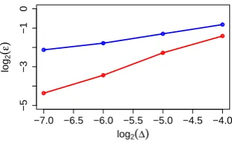
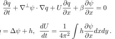
3.5.4 Quasi-Geostrophic Model on the β-plane with Mean Flow . . 50
Chapter 4 Estimating Parameters in Stochastic Differential Equation Models 60 4.1 Background . . . 61
4.2 Maximum Likelihood for the Ornstein-Uhlenbeck Process . . . 64
4.3 Approximations of the Likelihood Function . . . 68
4.3.1 Numerical Solutions of the Fokker-Planck Equation . . . 68
4.3.2 Particle Filters . . . 69
4.3.3 Importance Samplers . . . 69
4.3.4 Markov Chain Monte Carlo Methods . . . 73
4.3.5 Analytical Approximations of the Likelihood Function . . . . 81
4.3.6 Local Linearisation . . . 83
4.4 Exact Algorithms . . . 84
4.5 Alternatives to Likelihood Estimation . . . 87
4.5.1 Estimating Functions . . . 87
4.5.2 Generalised Method of Moments . . . 88
4.5.3 Estimation Via an Auxiliary Model . . . 89
4.6 Conclusion . . . 90
Chapter 5 Inference for Models with Cubic Drift and Linear Diffu-sion 91 5.1 Aspects of Bayesian Inference via Markov Chain Monte Carlo . . . . 93
5.2 Inference for Missing data . . . 96
5.2.1 Linear Bridge as a Proposal Process . . . 98
5.3 Inference for Diffusion Parameters . . . 112
5.3.1 Low dimensional noise . . . 117
5.4 Inference for Drift Parameters . . . 118
5.4.1 Gibbs Sampler . . . 119
5.6 Summary and Conclusions . . . 130
Chapter 6 Models with Latent Variables 133 6.1 Models with Latent Variables . . . 133
Chapter 7 Prediction for Models with Cubic Drift and Linear Diffu-sion 140 7.1 Derivation of the Stability Matrix . . . 141
7.1.1 Simple Models . . . 141
7.1.2 General Case . . . 143
7.2 Sampling the Stability Matrix . . . 145
7.2.1 Basic Algorithms . . . 145
7.2.2 Component-wise Sampling . . . 145
7.2.3 Central Wishart Algorithm . . . 150
7.2.4 Non-Central Wishart Algorithm . . . 154
7.2.5 Efficiency of the Algorithms . . . 155
7.3 Using a Stability Matrix as Prior . . . 159
7.4 Summary and Conclusions . . . 160
Chapter 8 Applications to Geophysical Models 164 8.1 Chaotic Lorenz System . . . 164
8.2 Model Reduction for Triad Systems . . . 171
8.2.1 Stochastic Mode Reduction . . . 172
8.2.2 Empirical Approach . . . 174
8.3 Model Reduction for the Quasi-Geostrophic Model with Mean Flow 177 8.3.1 Stochastic Mode Reduction . . . 178
8.3.2 Empirical Approach . . . 179
Chapter 9 Conclusions 183 Appendix A Example code for Empirical Climate Modelling 187 A.1 Main Program . . . 187
A.2 Sample Missing Data . . . 195
List of Tables
5.1 List of proposal distributions for Algorithm 4.2 that are studied and
tested in this chapter. . . 97
5.2 Diffusion parameter estimates for a two dimensional cubic model with
fixed drift function parameters given in Table 5.3. On the left is the true value of the parameter. The length of the data set used for
the inference is labelled as T and the observation interval is ∆ =
{0.1,0.01,0.001}. There was no missing data in this study. The
posteriors were estimated using 3×10⁶ samples from three MCMC
chains. In each cell the parameter is estimated from the posterior mean and in brackets is shown the 10-90 percentiles of the posterior.
The bottom of the table shows the Posterior Expected Loss of Eq.
(5.6). . . 117
5.3 Drift parameter estimates for a two dimensional cubic model with
fixed diffusion function parameters given by the values in Table 5.2
and no missing data. On the left is the true value of the parameter.
The length of the data set used for the inference is labelled as T
and the observation interval is ∆ ={0.1,0.01,0.001}. The posteriors
were estimated using 3×10⁶ samples from three MCMC chains. In
each cell the parameter is estimated from the posterior mean and in
brackets is shown the 10-90 percentiles of the posterior. The bottom
5.4 Drift parameter estimates for a two dimensional cubic model with
diffusion function parameters given by the values in Table 5.2. On the left is the true value of the parameter. The data used is the
same as that of Table 5.3 sampled at the ∆ = 0.1 interval. In this
case data is imputed to obtain the intervals ∆ ={0.01,0.001}. The
Modified Bridge sampler was used to impute data (see Table 5.1). The
posteriors were estimated using 3×10⁶ samples from three MCMC
chains. The bottom of the table shows the Posterior Expected Loss of Eq. (5.6). . . 123
7.1 Summary of Monte Carlo algorithms, discussed in this section, to
sample negative/positive definite matrices with Normally distributed components. . . 146
7.2 Model Problems for efficiency tests. Both are normal densities
Trun-cated Normal densities. The Normal distribution from which they are
derived has meanµ∈Rdand covarianceΓ∈
Rd×d. The components
of these densities are entered into the upper triangle of a matrixW
in row major order. Then it is required that W ∈Rp×p is negative
definite. Here we setd=p(p+ 1)/2 to be the number of independent
components. . . 150
7.3 The number of independent samples per second for the Monte Carlo
algorithms of Table 7.1 applied to model problem 1 of Table 7.2. The
results for the Rejection and Component-wise algorithm are
calcu-lated from the time taken to draw 106 samples; the remainder are
Markov Chain algorithms and so also include the efficiency factor as
described in the text. . . 158
7.4 The number of independent samples per second for the Monte Carlo
algorithms of Table 7.1 applied to model problem 2 of Table 7.2. The
results for the Rejection and Component-wise algorithm are
calcu-lated from the time taken to draw 106 samples; the remainder are
Markov Chain algorithms and so also include the efficiency factor as
List of Figures
2.1 Brownian Motion. Sample path of the process (left) and quadratic
variation as a function of log time interval (right). . . 12
2.2 Comparison of Euler and Milstein schemes for simulating the SDE in
Eq. (2.29). The Euler simulations are in blue and the Milstein in red. 23
3.1 Example of solution for triad model in Eq. (3.31) for= 0.1 withx1
shown in black andx2 in red. . . 46
3.2 Invariant distributions for variables in Eq. (3.31) for= 0.1. . . 47
3.3 Solution of the Galerkin truncation of the Burgers equation for times
t= 0,0.4,1.5,20 . . . 49
3.4 Evolution of Fourier amplitudes for k= 1,5,10,20 . . . 50
3.5 Example of dynamics of Mean flowUtfrom Eq. (3.40) . . . 54
3.6 Comparison of predicted density from equilibrium statistical
mechan-ics and the empirical density for the mean flow. . . 56
4.1 Maximum Likelihood Estimates for φin the O-U process model Eq.
(4.9). The blue (red) histogram are the estimates from the continuous (discrete) time model. The blue (red) curve is the asymptotic
distri-bution of estimates of the continuous (discrete) time model. The true
value is φ=−0.8. . . 66
4.2 Maximum Likelihood Estimates forσ2 in the O-U process model Eq.
(4.9). The blue (red) histogram are the estimates from the continuous (discrete) time model. The blue (red) curve is the asymptotic
distri-bution of estimates of the continuous (discrete) time model. The true
value is σ2 = 0.5. . . 67
5.1 Illustration of the inference problem. Red circles represent
observa-tions and blue are missing values to impute. The inclusion of missing
5.2 Sample paths of both components of the non-linear SDE (Eq. 5.15)
(black), the linear approximation (red) and the Brownian motion
(blue) using the same random variables. . . 99
5.3 Comparison of the distributions of the original process in Eq. 5.15
(black/grey) compared with contour plots of the linear approximation in Eq. (5.16) (red) and Brownian motion (blue) evolving from a fixed
initial condition for both components of Eq. (5.15). . . 100
5.4 Comparison of the distributions of the non-linear bridge process
de-rived from Eq. 5.15 (black/grey) compared with contour plots of the
modified linear bridge in Eq. (5.21) (red) and Brownian bridge (blue).
Here we usea= (3,2),b= (2,1) and= 0.1. . . 101
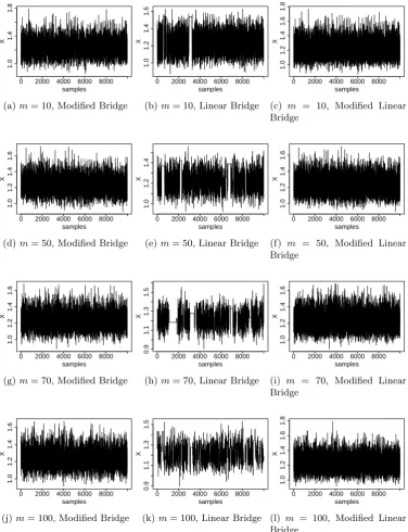
5.5 Trace plots of the MCMC output for sampling missing data from the
model in Eq. (5.23). The data shown is the average value for an
arbitrary observation interval with ∆ = 0.1. The Modified Bridge
is on the left, the Linear Bridge is centre and the Modified Linear
Bridge on the right. . . 103
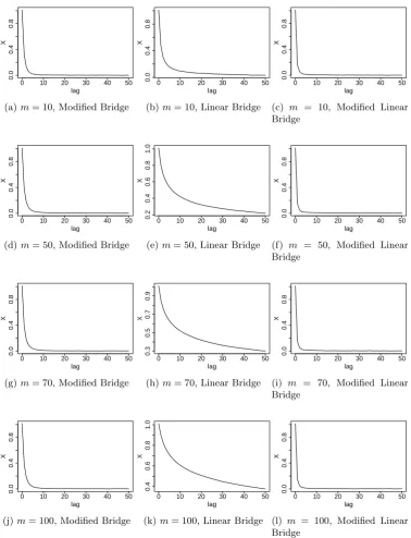
5.6 Average autocorrelation functions computed for MCMC output of
N = 100 data intervals from the model in Eq. (5.23) with
interobser-vation time ∆ = 0.1. The Modified Bridge is on the left, the Linear
Bridge is centre and the Modified Linear Bridge on the right. . . 104
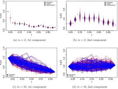
5.7 Output from Standard and Linear Bridge samplers applied to Eq.
5.24 in two dimensions observed at ∆ = 0.1. For each MCMC
al-gorithm 105 samples were retained after discarding a burn in of 104.
Plots (a) and (b) show a series of 11 observations overT = 1.0 with
imputed datam= 2. At each imputed data point the density of both
samplers is plotted using Kernel Density Estimation and the
“bean-plot” package in R. Plots (c) and (d) show the estimated densities for
the imputed data withm= 10 for a single observation interval. Also
shown are some sample paths from both MCMC algorithms. . . 105
5.8 Efficiency of different data imputation proposals described in the text:
BB - black, MB - red, LB - green, MLB - blue, BL - cyan, LL - ma-genta applied to the model in Eq. (5.24). In this case all components
X were updated simultaneously. The data consisted ofN = 101
sam-ples at observation interval ∆ = 0.1. Only missing data was sampled
in these algorithms. Each estimate of efficiency was calculated using
5.9 Efficiency of different proposals described in the text for the
componentwise updating: BB black, MB red, LB green, MLB blue, BL -cyan, LL - magenta applied to the model in Eq. (5.24). In this case
each component of X was updated separately. The data consisted
of N = 101 samples at observation interval ∆ = 0.1. Only missing
data was sampled in these algorithms. Each estimate of efficiency
was calculated using 105 samples from three MCMC chains after a
burn in of 104 samples. . . 111
5.10 Output of Random Walk algorithm for σ applied to the one
dimen-sional model in Eq. (5.27) with N = 101 observations,
interobserva-tion time ∆ = 0.1 and fixed α = 1.0. The true value was σ = 1.0.
On the right are the corresponding autocorrelation functions. Note
that the Modified Bridge Sampler was used to impute missing data
(see Table 5.1). . . 113
5.11 Output of Innovation Scheme for σ using the change of variables in
Eq. (4.38) and Eq. (4.39) applied to the same data set used in Figure
5.10. The Modified Bridge sampler was used to impute missing data (see Table 5.1). . . 115
5.12 Autocorrelation functions of Random Walk and Innovation Scheme
forσ1 applied to the six dimensional model in Eq. (5.27) with
obser-vation interval ∆ = 1.0. . . 116
5.13 Data set used for inference from Eq. (5.29). . . 118
5.14 Estimates of the posterior distributions of σ. Each curve is an
esti-mate of the posterior for a different amount of imputed data m. A
high frequency data set with N = 100 observations and
interobser-vation time ∆ = 1.0 from Eq. (5.29) was used. The true value is
σ = 1.0. On the left are the results from fitting the 1 dimensional
model Eq. (5.30) and on the right are those estimated from Eq. (5.29)
with 2-dimensional Brownian motion. . . 119
5.15 Output of Gibbs sampler for 20 drift parameters of two dimensional
model from Eq. (5.1). The observation interval is δ = 10−3 and
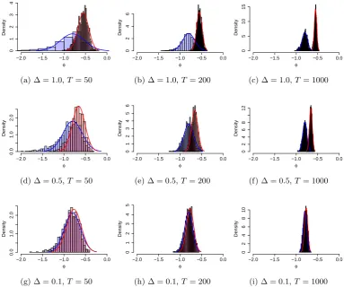
5.16 Marginal distributions of cubic parameters inferred for a two
dimen-sional model of form Eq. 5.1. A data set withN = 1,000 observations
at interval ∆ = 0.1 was used. The diffusion parameters were fixed and
there was no missing data. The blue histogram shows the parameters
that gave stable solutions to the SDE, while the mauve is for those that gave unstable solutions. The purple shows the overlap between
the two regions of the marginal distributions. The true values are
given by the red lines. . . 125 5.17 Posterior distributions for parameters from the O-U process Eq. (4.9)
output from the GPU implementation of Algorithm 5.1 (solid lines)
compared with the exact posterior distributions (histograms).
Pa-rameters were estimated using a data set withN = 100 observations
and interobservation time ∆ = 0.1. A single long run of 105 MCMC
samples were used to compute the posteriors. . . 129 5.18 Real computation times to draw 1000 MCMC samples from the
pos-terior distribution of the OU process for various size data sets. The
time in seconds is plotted versus the amount of missing data for an implementation of the algorithm on a CPU and GPU. . . 131
6.1 Data set from model Eq. (6.3) withN = 1000 points with observation
interval ∆ = 0.1. . . 138
6.2 Estimated posterior distributions for parameters from the latent
pro-cess model Eq. (6.3) for various amounts of imputed data m. . . 138
7.1 Left truncated normal distribution withµ− = 2 compared with scaled
optimal exponential proposal of Eq. (7.9) used for rejection sampling. 149
7.2 Doubly truncated normal distribution. The top figure hasu−= 2 and
u+= 3 and is better approximated with the exponential distribution.
The bottom figure hasu− = 2 andu+= 2.5 and the uniform is more
efficient. . . 150
7.3 Autocorrelation functions estimated from the output of the
Component-wise algorithm applied to Model Problem 1. They were estimated
using 105 MCMC samples after discarding an initial burn in of 104. . 151
7.4 Efficiency of the Wishart proposal distribution sampling the standard
normal distribution restricted to positive definite matrices (see text).
7.5 Output of non-central Wishart algorithm applied to model
prob-lem 2 in Table 7.2. The histograms are estimated from 105 MCMC
samples and the density in red from 105 samples drawn directly from
the distribution using theRejection algorithm. . . 156
7.6 Autocorrelation functions of non-Central Wishart algorithm
ap-plied to model problem 2 from Table 7.2. . . 157
7.7 Estimate posterior distributions for parameters from a two
dimen-sional model of the form Eq. (5.1) with N = 100 and ∆ = 0.1.
The parameters, which are randomly generated, are written in the
matrix notation introduced in Section 5.4.1. The histograms are the
posterior distributions with uninformative prior, in red are the pos-terior distributions for parameters with stable SDEs and in black are
the posterior distributions which include the stability matrix prior
information derived in this chapter. . . 161
8.1 Inference for the reduced double well model coupled to chaotic Lorenz
system: Eq. (8.1) for two values of . The stars show the value
σ2= 0.113 obtained by Mitchell and Gottwald [2012]. . . . 166
8.2 Predictive statistics for the reduced double well model coupled to
chaotic Lorenz system: Eq. (8.1) for two values of. In each plot the
lines correspond to the inferred one dimensional model for differentm.167
8.3 Posterior distribution estimates from MCMC output applied to a
sparse data set (∆ = 10). Distributions correspond to different
amounts of missing datambetween observations with the key shown
at the top. The distribution in brown, for m = 64, agrees with the
theoretical values predicted by the homogenisation procedure. . . 168
8.4 Quadratic variation, calculated as Eq. (8.4), for the processxt from
the model Eq. (8.1). The curves represent different time scale
sepa-rations. . . 170
8.5 Posterior estimates for parameters from the model Eq. 8.5 usingN =
1000 observations of Eq. (8.1) with observation interval ∆ = 0.01.
The posteriors were estimated using 105 samples from 3 chains after
discarding a burn in of 104 samples. The different posteriors are for
8.6 Plots comparing the autocorrelation function of the full chaotic Lorenz
model with reduced models. The bars are for the full model; red is the latent noise process; blue is the standard empirical model and
black is the theoretical model predicted by homogenisation. . . 171
8.7 Example of solutionx1 (black) andx2 (red) from the Burgers model
in Eq. (8.6) for two values of. . . 173
8.8 Posterior estimates of parametersσ and γ in Eq. 8.7 applied to data
simulated from Eq. (8.6) with= 0.8 for varying amounts of missing
data m. These distributions were estimated using 3×10⁵ samples
from Algorithms 4.1 and 4.2 using the Modified Bridge proposal. The
vertical black line is the mean of the posteriors estimated for the case
= 0.01 withm= 16. . . 174
8.9 Output statistics comparing the reduced model Eq. (8.7), with
pa-rameter estimates forσ and γ, for various with the full model. . . 175
8.10 Posterior estimates of drift parameters for two dimensional cubic
model Eq. (5.1) fitted toN = 5000 observations with interval ∆ = 0.1
of the triad-Burgers equation with= 0.8. 3×10⁵ MCMC samples
were retained after discarding a burn in of 104, from Algorithms 4.1
and 4.2 with the Modified Bridge proposal. The Gibbs sampler of
Section 5.4 was used to sample the matrixA shown here. . . 176
8.11 Autocorrelation plots of the full system in Eq. (8.6) with = 0.8
(vertical bars) and the empirical model Eq. 5.1) with parameters estimated as described in the text (red). . . 177
8.12 Results for inferring the one free parameter γ(10) in the one
dimen-sional reduced model in Eq. (8.8) to N = 1000 observations at
in-terval ∆ = 0.1 from the original system Eq. (3.40). On the left are
the posterior estimates, for varying missing data m, obtained using
3×10⁵ samples from Algorithms 4.1 and 4.2 with the Modified Bridge
proposal. On the right are the estimated autocorrelation functions of
the reduced model using the mean of the posterior estimate forγ(10)
with m = 16 compared to the simulation of the original model Eq.
8.13 Inference results for varying amounts of missing datamfor the cubic
model Eq. (8.10) fitted to N = 1000 observations of the mean flow
data with interval ∆ = 0.1. 3×10⁵ samples were used to estimate
these posterior distributions. Algorithm 4.1 was used to estimate
the two diffusion parameters (shown bottom), Algorithm 4.2 with the Modified Bridge proposal was used to impute the missing data
and the Gibbs sampler of Section 5.4 was used to infer the four drift
parameters ai, i= 1. . .4. . . 180
8.14 Predictive statistics for the mean flow using the inferred cubic model
Eq. (8.10) for varying missing datam. Top: stationary distributions
for various amounts of imputed data. The histogram is that of the
full system. Bottom: autocorrelation plots of the inferred model
List of Algorithms
4.1 Sample parameters entering the diffusion function. . . 80
4.2 Sample missing data between observations. . . 82
5.1 Parallel SDE inference with perfect observations. For each step Y
hasm+ 1 components and is stored in local memory, unique to each
thread. For the second step σ∗ is stored in shared memory so is
accessible to all threads. . . 128
7.1 Sample parameters along diagonal of Stability Matrix . . . 146
Acronyms
SDE Stochastic Differential Equation . . . 3
MCMC Markov Chain Monte Carlo . . . 3
ODE Ordinary Differential Equation . . . 7
FP Fokker-Planck . . . 14
PDE Partial Differential Equation . . . 14
LFV Low Frequency Variability . . . 24
PDF Probability Density Function . . . 25
EOF Empirical Orthogonal Function . . . 25
GCM General Circulation Model . . . 26
HMM Hidden Markov Model . . . 26
QG Quasi-Geostrophic . . . 26
OPP Optimal Persistence Pattern . . . 27
PIP Principal Interaction Pattern . . . 27
POP Principal Oscillation Pattern . . . 28, 40 CLT Central Limit Theorem . . . 29
MTV Stochastic Mode Reduction Strategy of Majda et al. [1999], Majda et al. [2001], Majda et al. [2009], Majda et al. [2002], Majda et al. [2003] . . . 35
OU Ornstein-Uhlenbeck . . . 40
LIM Linear Inverse Model . . . 40
ARMA Auto-Regressive Moving Average . . . 41
NH Northern Hemisphere . . . 41
MH Metropolis-Hastings algorithm . . . 73
PEL Posterior Expected Loss . . . 96
BB Brownian Bridge . . . 97
MB Modified Bridge . . . 97
LB Linear Bridge . . . 97
MLB Modified Linear Bridge . . . 97
BL Brownian Bridge Lamperti . . . 97
List of Symbols
d The number of components of a stochastic process . . . 7
∅ The empty set. . . 8
(Ω,F,P) A probability space . . . 8, 9 X A vector valued random variable . . . 8
ω An event in probability space Ω . . . 8, 9 x An observation of a random variable . . . 8
πX(U) A probability measure on set U ∈Rd, where d is the dimension of random variableX. . . 8
E[f(X)] The expectation of a function. . . 8
p(x) Probability density for x. . . 8
{Xt}t∈T A vector valued stochastic process indexed by timet. . . 8
t Timet∈T, whereT is an index set . . . 8, 9 xt An observation of stochastic process at timet. . . 9
Xt The path of a stochastic process, indexed by time t. . . 9
(Ω,F,P,{Ft}) A filtered probability space. . . 9, 16, 61 p(x1, t1|x2, t2;x3, t3,· · ·) Transition density for a process to evolve to state x1 at timet1 given the full path history, where t1> t2 > t3 >· · ·. . . 9
Bt Multivariate Brownian motion indexed by time t. . . 10
Rt
0 σ(Xs, s)◦dBs Stratonovich integration of functionf(X, s) with respect to
Brow-nian motionBs. . . .
12
µ(Xt, t) The drift function of a stochastic differential equation for X.. . . 12
a(Xt, t) The diffusion function of a stochastic differential equation for X. . . 13
θ The parameter vector entering the drift and diffusion function. . . 13
O(dt) The order of a quantity dt. . . 13
L2(P) Space of square integrable functions with respect to probability space (Ω,F,P).
13
Σ(x, t) The covariance matrix of the processxat timet. . . 14
mb Shorthand for millibar. One thousandth of the unit of atmospheric pressure,
the Bar=100,000 pascals. . . 25
Small parameter quantifying time scale separation. . . 29
· Inner product between vectors, a·b=P
iaibi. . . 31
: Inner product between matrices,A:B =P
ijAijBij. . . 31
⊗ Outer product between matrices, whereA,B ∈Rm×d⇒A⊗B∈
Rm×msatisfies
(A⊗B)c=ABTc. . . 34
hPa Hecto-Pascal = 100 Pa. . . 41
∆tk Forward observation interval ∆tk=tk+1−tk. . . 62
∆ Constant inter-observation time. . . 64
m Partition of interval into m−1 sub-intervals. . . 70
δ Constant sub-interval timeδ= ∆/m. . . 70
µk Shorthand for the drift functionµ(ξk,θ). . . 70
Acknowledgments
Many thanks to my two supervisors Dr Christian Franzke at the British Antarctic
Survey (BAS) and Professor Gareth Roberts of Warwick Statistics. Also I would
like to express my appreciation for the training provided by the Complexity
Sci-ence Doctoral Training Centre and the friendly support of the students, lecturers
and administrators. Add to this Warwick’s Centre for Scientific Computing, whose
facilities I used extensively during this work, particularly the high performance
clus-ter Minerva. Many thanks to the EPSRC for providing the main funding for this
research. Thanks also to support from NERC, who provided my travel and
accom-modation expenses to visit Dr Franzke at BAS. Special thanks to my wife Charlotte
Declarations
The work presented here is my own, except where stated otherwise. This thesis
has been composed by myself and has not been submitted for any other degree or
professional qualification.
• The majority of computer code for this thesis was written by myself. Examples
of this code can be found in the Appendix and all parts can be requested by
email. I acknowledge Koev and Edelman [2006] for making available their code
for computing the Hypergeometric Function of a Matrix Argument (Written:
May 2004). The program also relies upon the GNU scientific library.
Ad-ditional code was provided by Dr Franzke to simulate the quasi-geostrophic
model.
• All data in this thesis were produced by simulations conducted by myself.
• The analytical results in Chapter 3 are known, but all derivations were
per-formed independently by myself.
• The findings of Chapter 8 regarding best practice in stochastic climate
mod-elling including the use of latent noise processes will be submitted for
publi-cation.
• The study of improved proposal distributions for missing data in Chapter 5
Abstract
This thesis is about the construction of low dimensional diffusion models of climate
variables. It assesses the predictive skill of models derived from a principled
averag-ing procedure and a purely empirical approach. The averagaverag-ing procedure starts from
the equations for the original system then approximates the “weather” variables by a
stochastic process. They are then averaged with respect to their invariant measure.
This assumes that they equilibriate much faster than the climate variables. The
empirical approach argues for a very general model form, then parameters are
esti-mated using likelihood based inference for Stochastic Differential Equations. This is
computationally demanding and relies upon Markov Chain Monte Carlo methods.
A large part of this thesis is focused upon techniques to improve the efficiency of
these algorithms.
The empirical approach works well on simple one dimensional models but
performs poorly on multivariate problems due to the rapid increase in unknown
parameters. The averaging procedure is skillful in multivariate problems but is
sensitive to lack of complete time scale separation in the system. In conclusion,
the averaging procedure is better and can be improved by estimating parameters in
a principled way based on the likelihood function and by including a latent noise
Chapter 1
Introduction
The Earth’s climate is a complex system consisting of several coupled sub-components such as the atmosphere, oceans, biosphere and cryosphere (glaciers, sea ice and
snow), which evolve on different time scales. The deterministic equations
govern-ing the physics of these systems are derived from the classical laws of mechanics, thermodynamics and fluid flow. In the case of the atmosphere, the dynamics are
governed by the non-linear Navier-Stokes equations for compressible flow on a
ro-tating sphere. Together with the equation of state, and conservation of mass and energy, they determine the changes in velocity, temperature, pressure and density,
as well as the amount of water vapour in the air. Fundamentally, it is these
equa-tions which must be solved to provide weather predicequa-tions or climate simulaequa-tions. However, the Navier-Stokes equations are much too detailed for climate prediction
as they resolve processes with length scales ∆x = O(10−3m) and time scales as
small as ∆t=O(10−1s). They include a range of processes from sound waves, with
time scales of milliseconds, to the thermohaline circulation of the ocean.
Whether simulating the full climate system or making short term weather
predictions, whatever the time scale of interest, approximations are made, which express the fields of interest as composed of an average component and small high
frequency perturbations from this balanced state. The model is simplified by
fil-tering out the high frequency variability. Due to the interaction between different scales in the system the averaged equations are not closed with respect to the high
frequency fields. Closed equations are obtained by introducing a parametrisation: a
law that specifies the effects of the unresolved processes on the large scale dynam-ics. Parametrisations could be based on a physical or empirical relation. Examples
major source of error in a simulation.
A parametrisation can be considered a statistical mechanics treatment of the system. Macroscopic quantities arise as the most likely state given the ensemble
of microstates which are distributed according to some stationary probability
dis-tribution. More usefully one can employ a mesoscopic treatment of the sub-grid scale processes. Then we allow the probability distribution of microstates to evolve
in time governed by some PDE. Now our macroscopic quantity obeys a stochastic
process akin to a Brownian particle buffeted by invisible fluid particles.
Stochastic parametrisation is a method of including model uncertainty in our
predictions. Alternatively, we can consider the initial condition uncertainty due to
our imperfect observations of the system. One can consider the initial conditions as random variables with a known probability distribution. This randomness then
propagates into the solution. This has implications for predictability since the
at-mosphere is a highly non-linear chaotic system. Systems evolving from different initial conditions can have diverging solutions and so one simulation may not
cap-ture the full range of possible dynamics given our knowledge of the initial state. It
is therefore useful to perform an ensemble of simulations with varying initial condi-tions. This is done routinely at the European Centre for Medium Range Weather
Forecasting.
Given the importance of climate science in preparing humanity for a changing
future and the role that weather prediction plays in everything from insurance claims
to the price of energy it is vital that Earth system research continues to make improvements in the predictive skill of models. Improvements in parametrisations,
finer grid resolutions and the use of satellite data to initialise weather simulations
have made great progress. However, there is a growing appreciation that, due to the scale invariance of the system, sub grid scale processes will always be important
and the error can not be reduced to zero. This motivates further study of stochastic
parametrisations and stochastic modelling in climate science with a view towards the probabilistic Earth-System Simulator. At least with this we will have an accurate
estimate of our prediction uncertainty.
1.1
Aims of this Thesis
This thesis is about low dimensional stochastic modelling of atmospheric systems.
The closure problem discussed above introduces stochastic terms and unknown pa-rameters into these models. This thesis focuses on the problem of statistical
we research and develop suitable methodology to estimate the unknown parameters
from time series observations of the system. Specifically we work with Stochastic Differential Equations (SDEs).
Although this empirical approach to constructing SDEs for atmospheric
pro-cesses has been done in the literature in several ways we focus on the difficult statistical problem of likelihood based inference. This is challenging because
non-linearity of the models forces an approximation of the likelihood function.
Funda-mental results show that this approximation converges to the true likelihood as the observation interval goes to zero. However, this is not necessarily obtained by a real
data sampling strategy.
In order for the methods to be useful in practice we consider the scenario of infrequent observations. In this case the literature suggests augmenting the data
by repeatedly simulating additional points between observations, adopting a
Monte-Carlo strategy to integrate over the missing data. Maximum likelihood estimation is difficult in this case due to the noise introduced by the Monte Carlo method
leading to a non-convex optimisation. Instead we use a Bayesian approach. We
aim to estimate the posterior distribution of the unknown parameters given the observations and the additional uncertainty introduced by the missing data. We
now have an integration rather than a maximisation problem.
One of the aims of this thesis is to continue the research into efficient Markov
Chain Monte Carlo (MCMC) methods for this problem. Specifically, we investigate
the performance of missing data sampling strategies as the dimension of the system increases. We also consider the problem of poor mixing of MCMC due to the
de-pendency between missing data and diffusion parameters. We review the literature
of methods proposed to tackle this problem and compare them with other MCMC strategies.
One issue is the computational effort required in the inference of
multi-dimensional systems. We aim to implement efficient code written in a low level language such as C/C++. We also assess the performance gains from using
mas-sively parallel computation with Graphics Processor Units (GPUs).
One problem encountered early in the research was that the subset of param-eter space leading to a stable SDE becomes small as the dimension of the system
increases. A lot of the posterior mass was on parameter values which lead to
solu-tions exploding to infinity in finite time. Predicsolu-tions from these models are obviously not useable. The Bayesian approach is useful because we can include prior
infor-mation about parameters which restricts them to the subspace leading to stable
included and how it affects the inference strategy.
We aim to assess a current stochastic modelling strategy which predicts the functional form for the reduced model but introduces several parameters which
must be estimated from data. We apply our inference algorithm to these unknown
parameters. A crucial working assumption of this method is that there exists time scale separation between resolved and unresolved modes of the system. We aim to
assess the performance when there is imperfect separation of time scales. To do this
we use a series of toy models, starting with those where the time scale separation is explicit and known, then moving to more sophisticated models of geophysical
dynamics where time scale separation is an assumption. We aim to use consistent
measures of predictive skill to determine the ability of reduced models to reproduce the statistics of the full. Finally we aim to apply our methods to data from a
sophisticated atmospheric model.
1.2
Outline of this Thesis
This thesis is broadly divided into methods (Chapters 4 and 5-7) and applications
(Chapters 3 and 8) although, firstly, in Chapter 2 we present some theory of
Stochastic Differential Equations (SDEs). We briefly recap some properties of
Brow-nian motion and diffusion processes. We state some useful results regarding the
existence and stability of solutions of SDEs, which will be used later to restrict the parameter space through prior information. We also discuss the Girsanov change
of measure theorem which is crucial to understanding likelihood based inference for
SDEs and the problems that arise. We introduce bridge processes which will be used as part of the inference methods in Chapters 4 and 5.
In Chapter 3, we review the existing literature on stochastic modelling in climate science. Here we discuss how the field developed from Hasselmann’s seminal work of 1976 and the successful application of these ideas to the understanding of the
El Nino system. We also review more recent work on low dimensional modelling of
the atmosphere and the methods of statistical inference that have been employed. In this Chapter we also introduce some of the mathematical theory of averaging
and homogenisation which underpins the stochastic mode reduction strategy that
motivates this thesis. We then present the three toy problems with which we will work, and derive reduced models for each case.
Chapter 4builds upon the theory of Chapter 2 applied to the inference prob-lem. We discuss the literature, briefly mentioning non-likelihood based approaches
key contributions from the literature regarding likelihood based inference and in
par-ticular on the Bayesian approach and Markov Chain Monte Carlo (MCMC) meth-ods. We demonstrate the potential problems encountered with naive algorithms and
review more sophisticated methods. We argue for a particular flexible algorithm,
taken from the literature, as suitable for our applications and we give details of the implementation.
InChapter 5 we focus on improving the efficiency of MCMC methods ap-plied to our particular class of model. We introduce the use of the multivariate non-time homogeneous linear bridge as an efficient method to propose missing data.
We discuss sampling diffusion parameters and the difficulty associated with models
having low dimensional noise. We present a Gibbs sampler for the drift parame-ters and investigate the computational improvements gained from using Graphics
Processing Units for sampling diffusion parameters.
SDEs driven by red noise are one possibility for modelling systems with lack of time scale separation. This introduces latent, unobserved processes into the SDE
model. Inference methods for imputing latent processes are derived inChapter 6.
InChapter 7 we discuss the problem of restricting the parameter space in order to obtain stable SDEs and we present one method of solving this problem.
From this arises the problem of inference for positive definite matrices. We present several algorithms which tackle this problem, one of which is based on a novel use
of the non-central Wishart distribution.
In Chapter 8we apply our methods to a range of toy problems which, to varying degree, represent the type of non-linear dynamics with time scale
separa-tion one could expect from the atmosphere. We start with double well dynamics,
coupled to the chaotic Lorenz system. We compare the cubic models, with parame-ters inferred empirically, with the theoretically motivated model resulting from the
homogenisation procedure. The next step is to consider a bivariate model. For
this we consider a triad model coupled to a the Burgers equation. We then move onto a model with more realistic features of atmospheric flow, namely the
Quasi-Geostrophic Model on the Beta Plane with mean flow. In this case the time scale
separation is not explicitly known. In each case we compare the stationary proba-bility density and autocorrelation functions of the reduced model with the full. We
Chapter 2
Stochastic Differential
Equations
In this thesis we work extensively with Stochastic Differential Equations (SDEs). In
this Chapter we will collect some definitions and results needed to work with SDE
models and that will be required for the rest of the thesis. The Chapter is largely based upon the books by Øksendal [2007], Gardiner [2004] and Kloeden and Platen
[1992].
SDEs are a widely used modelling framework. They continue to be
exten-sively used in mathematical finance since the seminal work of Black and Scholes
[1973] on option pricing and have been used in equilibrium economics as models of interest rates [Cox et al., 1985]. Techniques for fitting nonlinear models have been
developed and applied to the Eurodollar exchange rate [Elerian et al., 2001] and
stock prices [Bibby and Sorensen, 2001]. Stochastic volatility models have become popular to capture the time dependent noise in stocks; methods for fitting
mod-els with latent, unobserved processes have therefore been developed [Eraker, 2001].
Rigorous treatment of topics in mathematical finance, including option pricing and optimal control, is given by Karatzas and Shreve [1997]. The extension to modelling
markets with jumps (diffusions with discontinuous paths) is given in Øksendal and
Sulem [2007].
In physics, SDEs have been used in the development of non-equilibrium
sta-tistical mechanics since the early 20th century. They are used to describe the time
dependence of fluctuations in macroscopic quantities such as pressure and energy in a system with an enormous number of variables [van Kampen, 1997]. Einstein derived
an equation to describe the old problem of Brownian motion of a particle in a fluid
of individual particles. The resulting Langevin equation (or the Ornstein-Uhlenbeck
model [Uhlenbeck and Ornstein, 1930]) has now been generalised for nonlinear mod-els [van Kampen, 1981; Ramshaw, 1985]. Specific applications include molecular
dynamics [Feller et al., 1995; Gordon et al., 2009; Pokern et al., 2009; Hegger and
Stock, 2009], chemical reaction dynamics [Gillespie, 2000], quantum mechanics [Ford et al., 1988; Olavo et al., 2012], neuron firing [Ota et al., 2009], nuclear fission [Abe
et al., 1996] and turbulence [POPE, 1994].
Applications in medicine and biology include modelling gene regulatory net-works [Golightly and Wilkinson, 2005, 2008], molecular reaction netnet-works [Sjberg
et al., 2005], nonlinear models in epidemiology [Chen and Bokka, 2005], modelling
the growth of blood vessels in tumours [Capasso and Morale, 2009] and population genetics [Fearnhead, 2006].
Examples in Earth Sciences include the work of Ditlevsen [1999] on modelling
sudden climate change observed in ice core data; modelling drought and flood risk using SDEs [Unami et al., 2010]; stochastic modelling of soil salinity [Suweis et al.,
2010]; stochastic parametrisations of unresolved processes in climate models [Wilks,
2008] and hedging climate risk exposure using financial markets [Chaumont et al.,
2006]. A lot of work has been done on modelling fast chaotic processes in the
atmosphere as noise, resulting in an SDE model for the slow variables (see for example Franzke et al. [2005]). This is closely related to the work in this thesis and
the associated literature will be reviewed in Chapter 3.
An SDE is an extension of an Ordinary Differential Equation (ODE) to
include a random component. Consider extending addimensional ODE system to
include a random component as in
dXt
dt =µ(Xt, t) +a(Xt, t)Wt, X0=x0, X ∈R
d (2.1)
where µ : Rd×R+ → Rd, a : Rd×R+ → Rd×m and Wt ∈ Rm is a standard
Gaussian white noise. Solutions to this equation can be written, formally, as
Xt=x0+
Z t
0
µ(Xs, s)ds+
Z t
0
a(Xs, s)Wsds . (2.2)
2.1
Some Mathematical Preliminaries
Here we recall some concepts related to random variables and stochastic processes,
fixing the notation for the thesis. For further details refer to Øksendal [2007]. If Ω is
a set then aσ-algebraF on Ω is a collection of subsets with the following properties
• ∅ ∈ F
• F ∈ F ⇒FC ∈ F, whereFC is the compliment of F
• A1, A2, . . .∈ F ⇒A=∪∞i=1Ai ∈ F
The pair (Ω,F) is called a measurable space. A probability measurePon (Ω,F) is
a functionP:F →[0,1] such that
• P(∅) = 0
• P(Ω) = 1
• IfA1, A2, . . .∈ F and {Ai}∞i=1 is disjoint then
P(∪∞i=1Ai) =
∞
X
i=1
P(Ai).
The triple (Ω,F,P) is called a probability space.
Addimensional random variableXis a function from the probability space
to thed dimensional real numbers X : Ω → Rd. To denote an observation of the
random variable we use the informal notationX(ω) =x, whereω ∈Ω is an event.
For each Borel setU ⊂Rda random variable induces a probability measure, defined
by
πX(U) =P(X−1(U)).
πX(U) is called the distribution of X. The expectation of a function is defined
E[f(X)] =
Z
Rd
f(x)dπX(x)
In this thesis we work with probability measures that have a density p(x) with
respect to Lebesgue measure so that
E[f(X)] =
Z
Rd
f(x)p(x)dx.
A stochastic process {Xt}t∈T ∈ Rd, on probability space (Ω,F,P), is a
timet we have an observation functionxt:ω →Xt(ω), ω ∈Ω. For fixedω ∈Ω we
call the functionXt:t→Xt(ω) the path of the stochastic process.
Relevant for later theory in Section 2.5 and the literature review in Chapter
4 are the concepts of afiltered probability spaceand amartingale. A filtration,
on measurable space (Ω,F), is an increasing family of σ-algebrasFt⊂ F so that
0≤s < t⇒ Fs⊂ Ft.
We use the notation (Ω,F,P,{Ft}) to refer to a filtered probability space. A d
-dimensional stochastic process {Xt} on (Ω,F,P) is a martingale with respect to
filtrationFtif
• Xt is Ft-measurable for allt
• E[|Xt|]<∞for all t
• E[Xt|Xs] =Xs for all t≥s,
where the expectations are taken with respect toP.
Associated with a stochastic process is a transition probability density,
de-fined by
P(Xt∈A|Xs=xs) =
Z
y∈A
p(t,y|s,x)dy.
In general a stochastic process can depend upon its full path history so
that the transition probability density to be in state x1 at time t1, is written
p(x1, t1|x2, t2;x3, t3,· · ·), where t1 > t2 > t3 > · · ·. We say that the process is
Markovif
p(x1, t1|x2, t2;x3, t3,· · ·) =p(x1, t1|x2, t2), (2.3)
i.e the transition density only depends upon the current state. In real systems, observations at fine intervals are likely to depend upon some of the recent history.
However, a Markov process may be appropriate on the time scale we are interested
in and is a useful modelling framework.
In this thesis we will only consider stochastic processes with continuous
sam-ple paths. This excludes models with jumps that are gaining popularity in finance.
A sample path is continuous if it satisfies theLindeberg condition
lim ∆t→0
1
∆t
Z
|x−z|>
dxp(x, t+ ∆t|z, t) = 0, (2.4)
where > 0. This states that the probability for x to be finitely different from z
2.2
Brownian Motion and the Ito Integral
Now that we have introduced notation for stochastic processes we can consider
an important example. Brownian motionwas first proposed as a model for the
movement of pollen grains undergoing “random” movements. This has been studied
mathematically as a stochastic process and generalised to ddimensions. Here, we
recap some of the theoretical properties of mathematical Brownian motion that will allow is to understand and evaluate integrals such as the one in Eq. (2.2). With
regards to Eq. (2.2) we introduce the notationdBt=Wtdt. The stochastic process
given by
Bt=
Z t
0
dBs
is known as standard Brownian motion and has the following properties
1. B0 = 0
2. Almost surely continuous pathsBt
3. Independent, stationary increments
4. Bt−Bs∼ N(0, t−s),0≤s≤t
Sometimes referred to as the Wiener process, its existence was proved by Wiener [Wiener et al., 1966]. We state some of the key facts that allow one to integrate
with respect to Brownian motion.
The first integral in Eq. (2.2) is to be understood in the usual Riemann-Stieltjes sense. To appreciate why the second integral can not be treated this way
consider the one dimensional problem of computing
Z 1
0
BsdBs. (2.5)
First define the step function as any function that can be written as
f(x) =
n
X
i=0
αiIAi(x),
whereαiare real numbers,Aiare intervals andIis the indicator function (I[t1,t2](t) =
1 ift1 ≤t < t2,0 otherwise). Approximating the integrand in Eq. (2.5) as the step
function over the interval [0,1] as
B(t, ω)≈f1(n)(t, ω) = 2n−1
X
j=0
the integral has expected value
E
Z 1
0
f1(n)(s, ω)dBs(ω)
= 2n−1
X
j=0
E[Bj2−n(B(j+1)2−n−Bj2−n)] = 0.
Here we have used the independence of the increments of Brownian motion.
Alter-natively, if the integrand is approximated as
B(t, ω)≈f2(n)(t, ω) = 2n−1
X
j=0
B(j+1)2−nI[j2−n,(j+1)2−n](t), (2.7)
then we get
E
Z 1
0
f2(n)(s, ω)dBs(ω)
= 2n−1
X
j=0
E[B(j+1)2−n(B(j+1)2−n−Bj2−n)]
= 2n−1
X
j=0
E[(B(j+1)2−n−Bj2−n)2]
= 2n−1
X
j=0
2−n= 1,
where we have used properties 3 and 4 of standard Brownian motion. This example
shows that the integral depends upon which point of the interval [j2−n,(j+1)2−n) we
choose to approximate the function, unlike the Riemann integral which converges
regardless of the point chosen. This phenomenon is due to the large increments of the Brownian motion path; it can be shown that Brownian motion is nowhere
differentiable [Øksendal, 2007]. Also, the total variation of almost all Brownian
motion sample paths over an interval [s, t] is unbounded, i.e
lim ∆tk→0
X
s≤tk<t
|Bti+1−Bti|=∞, (2.8)
Since the integrator dBt is not a bounded variation process the Riemann-Stieltjes
interpretation of the integral does not necessarily exist [Øksendal, 2007]. However,
Brownian motion has finitequadratic variation, given by
lim ∆ti→0
X
s≤ti<t
(Bti+1−Bti)
2= (t−s) inL2. (2.9)
0 2 4 6 8 10
−1.0
0.0
1.0
2.0
t
Bt
● ● ● ● ● ● ● ● ● ● ● ●
−10 −8 −6 −4 −2 0
6
7
8
9
10
log2(∆)
Quadr
atic V
ar
iation
Figure 2.1: Brownian Motion. Sample path of the process (left) and quadratic variation as a function of log time interval (right).
defined even though different for each choice of approximation. Figure 2.1a shows
a sample path of Brownian motion over the time interval [0,10]. Figure 2.1b shows
the quadratic variation converging to the value in Eq. (2.9) as the discretisation interval goes to zero.
Integration with respect to Brownian motion depends upon the point where
the integrand is approximated. Choosing the left point t∗j = tj, as in Eq. (2.6),
leads to theIto integral, denoted
Z t
0
σ(Xs, s)dBs= lim
n→∞
X
j
f(Xtj, tj)(Bj+1−Bj),
Another common choice is to uset∗j = (tj+1−tj)/2, the mid point of the interval.
This is called theStratonovich Integraland is written
Z t
0
σ(Xs, s)◦dBs= lim
n→∞
X
j
f(X(tj+1−tj)/2,(tj+1−tj)/2)(Bj+1−Bj).
There are different cases where each integral is more appropriate and there exist relations between the two.
In this thesis we write Eq. (2.1) in the standard notation for SDEs
dXt=µ(Xt, t)dt+a(Xt, t)dBt ,X0=x0, (2.10)
where in general the Brownian motion may be of different dimension to X, so
that X ∈ Rd,B ∈ Rm, µ : Rd×[0,∞) → Rd and a : Rd×[0,∞) → Rd×m. It
is understood that the second term is integrated in the sense of Ito. Eq. (2.10)
function and a(Xt, t) as the diffusion function. We will usually work with
autonomous SDEs, where there is no explicit time dependence in the drift and diffusion functions. It is also often useful to write the drift and diffusion function’s
dependence on a parameter vector θ explicitly. Those cases where there is split
between the components entering the drift and diffusion functions we write θ =
{γ,σ}and the SDE in Eq. (2.10) is written
dXt=µ(Xt,γ)dt+a(Xt,σ)dBt X0 =x0. (2.11)
In contexts where we want to emphasize a function’s dependence upon the
under-lying probability space we write, for example,a(t, ω) to mean a(Xt(ω),σ).
2.3
Ito’s Formula
Ito’s formula is the SDE analogue of the chain rule. It is a key tool when working
with SDEs and in particular is needed to integrate equations like Eq. (2.11). Ito’s
formula is a rule for changing variables when working with SDEs. It is used to
determine the governing equation for a smooth functionf :Rd×[0,∞)→Rp.
LetY =f(Xt, t) then expanding the differential to second order we have
dYk=
∂fk
∂t (Xt, t)dt+ X
i
∂fk
∂xi
(Xt, t)dXi+
1 2
X
i,j
∂2fk
∂xi∂xj
(Xt, t)dXidXj. (2.12)
In the usual chain rule only the first two terms are of order O(dt). The third term
isO(dt2) and not included. In the case of SDEs, if we substitute the expressions for
dXi from Eq. (2.11) into the third term we get terms of the form dBidBj. These
are retained as they are of orderO(dt). To see this consider property 4 of Brownian
motion: the variance of an increment ∆Bj is equal to the time difference ∆tj. One
can derive rigorously that
X
j
f(Xj, tj)(∆Bj)2→
Z t
0
f(Xs, s)ds inL2(P) as ∆tj →0.
calculate theO(dt) terms fromdXidXj in Eq. (2.12) gives
dYk=
∂fk
∂t (Xt, t)dt+ X
i
∂fk
∂xi
(Xt, t)µi(Xt, t) +
1 2
X
i,j,l
∂2fk
∂xi∂xj
(Xt, t)ailajl
dt
+X
i,j
∂fk
∂xi
(Xt, t)aij(Xt, t)dBj. (2.13)
Ito’s formula can be used to compute integrals such as Eq. (2.5). Using the
change of variablesYt=Bt2 we have
dBs2 = 2BsdBs+
1
22ds .
Then
Z t
0
BsdBs=
Z t
0
(dB2s−ds) =Bt2−t , (2.14)
so that the integral differs from the equivalent finite variation process by the factor −t.
2.4
The Fokker-Planck Equation
The Fokker-Planck (FP) is a Partial Differential Equation (PDE) for the time
evo-lution of the transition density of a SDE (see Gardiner [2004]). In Chapter 3 it is used to derive the reduced dimensional climate model.
Consider SDE of the form Eq. (2.11). IfΣ(x, t) =aT(x, t)a(x, t) is the
co-variance matrixof the process then the Fokker-Planck equation for the transition density is
∂p(x, t|z, t0)
∂t =− X
i
∂ ∂xi
µi(x, t)p(x, t|z, t0)
+1
2
X
i,j
∂2
∂xi∂xj
Σij(x, t)p(x, t|z, t0)
,
(2.15)
where we have
µi(x, t) = lim
∆t→0
Z
Rd
(zi−xi)p(z, t+ ∆t|x, t)dz (2.16)
and
Σi,j(x, t) = lim
∆t→0
Z
Rd
(zi−xi)(zj−xj)p(z, t+ ∆t|x, t)dz. (2.17)
Solutions of the equation arediffusion processes. This equation defines thedrift
and (2.17) respectively, connecting the stochastic differential equation and diffusion
descriptions of the same system. The Fokker-Planck equation is known in
mathe-matics as theForward Kolmogorovequation.
For insight, and to demonstrate an application of Ito’s formula, we provide
a derivation of the Fokker-Planck equation for a 1 dimensional process. Using Ito’s formula, consider the time evolution of the expectation of an arbitrary twice
con-tinuously differentiable function f(X(t)), where X(t) is the process in Eq. (2.11)
with initial conditionX(0) =y. Taking expectations with respect to the transition
density we have
dE[f(x(t))]
dt = Z
dxf(x)∂p(x, t|y, t0)
∂t
=E
df(x(t))
dt
=E
µ(x, t)∂f
∂x +
1
2a(x, t)
2∂2f
∂x2
=
Z dx
µ(x, t)∂f
∂x+
1
2a(x, t)
2∂2f
∂x2
p(x, t|y, t0)
=
Z
dxf(x)
−∂[µ(x, t)p(x, t|y, t0)]
∂x +
1 2
∂2[a(x, t)2p(x, t|y, t0)]
∂x2
,
where we have used integration by parts, discarding surface terms. Since f(x) is
arbitrary we have, with the appropriate initial condition p(x, t0|y, t0) = δ(x−y),
the Fokker-Planck equation in 1 dimension
∂p(x, t|y, t0)
∂t =−
∂[µ(x, t)p(x, t|y, t0)]
∂x +
1 2
∂2[a(x, t)2p(x, t|y, t0)]
∂x2 . (2.18)
It is sometimes easier to work with thebackward Fokker-Planckequation
[Gar-diner, 2004]:
∂p(x, t|y, t0)
∂t =− X
i
µi(y, t0)
∂[p(x, t|y, t0)]
∂yi
−1
2aij(y, t0)
2∂2[p(x, t|y, t0)]
∂yi∂yj
. (2.19)
The difference is that now the variables x at time t are fixed and y varies. Eq.
(2.19) is also referred to as thebackward Kolmogorov equation. We will use it
2.5
Girsanov’s Change of Measure Theorem
Intuitively Girsanov’s theorem states that if we change the drift of an Ito
diffu-sion then the law of the new process will be absolutely continuous with the law of the original process. Girsanov’s theorem is extensively used for option pricing in
mathematical finance. It is also central to likelihood based inference for diffusion
processes, discussed in detail in Chapter 4.
LetXtbe an Ito process, on filtered probability space (Ω,F,P,{Ft}), of the
form
dXt=µ(t, ω)dt+dBt. (2.20)
LetMt be given by
Mt(ω) = exp
−
Z t
0
µ(s, ω)dBs−
1 2
Z t
0
µT(s, ω)µ(s, ω)ds
.
TheNovikov condition
E
exp
1 2
Z t
0
µT(s, ω)µ(s, ω)ds
<∞,
is sufficient to guarantee that this is a martingale with respect to the filtration
Ft (see Øksendal [2007]). If P is the law associated with process (2.20) then the
Girsanov transformation gives a new measure onFt by
dQ(ω) =Mt(ω)dP(ω).
and the process Xt is a Brownian motion with respect to Q. The theorem implies
that for all setsF1, . . . , Fk ⊂Rand all t1, . . . , tk≤t we have
Q(Xt1 ∈F1, . . . ,Xtk ∈Fk) =P(Bt1 ∈F1, . . . ,Btk ∈Fk).
Equivalently we can say thatQis absolutely continuous with respect to P, written
PQ. Then we can write
dQ
dP =Mt on Ft.
and callMt theRadon-Nikodym derivative of Qwith respect toP.
For the lawPa of a SDE with general diffusion function
the Radon-Nikodym derivative is
dQa
dPa
(ω) = exp
−
Z t
0
µT(s, ω)a−1(s, ω)dWs−
1 2
Z t
0
µT(s, ω)a−1(s, ω)µ(s, ω)ds
= exp
−
Z t
0
µT(s, ω)a−1(s, ω)dXs+
1 2
Z t
0
µT(s, ω)a−1(s, ω)µ(s, ω)ds
.
(2.21)
This ratio serves as the likelihood function for the parameters entering the drift function. However, the Radon-Nikodym derivative between measures induced by
diffusions with differing diffusion functions does not exist. This is because they do
not have the same sets of measure zero: they aremutually singular. As discussed
further in Chapter 4 one can not use Eq. (2.21) as the likelihood for inferring
parameters in the diffusion function as there is no common dominating measure. Therefore, it is sometimes useful to transform a SDE to one of unit diffusion (so
all unknown parameters are in the drift function) before performing inference. This
can be done using theLamperti Transform. Consider the one dimensional SDE
dXt=µ(X, t)dt+a(Xt)dBt, Xt0 =x0
and let
Yt=g(Xt) =
Z Xt du
a(u). (2.22)
Then, using Ito’s formula,Ytsatisfies the SDE
dYt=
µ(g−1(Yt), t)
a(g−1(Yt))
−1 2
∂a ∂x(g
−1(Y
t))
dt+dBt, Yt0 =g(x0),
which has unit diffusion. However, this transformation can not be performed for
general multivariate diffusion. The change of variableg is the solution of ∇g(x) =
a−1(x). A solution exists if the inverse ofais a gradient, i.e
∂[a−1]ij(x)
∂xk
= ∂[a
−1]
ik(x)
∂xj
(2.23)
for all triples i, j, k= 1, . . . , n, wherenis the dimensionality [Ait-Sahalia, 2008].
2.6
Existence, Uniqueness and Stochastic Stability
Here we state some qualitative results about the solution to SDEs such as Eq. (2.11).