Lane formation by side stepping

Original citation:

Burger, Martin, Hittmeir, Sabine, Ranetbauer, Helene and Wolfram, Marie-Therese. (2016)

Lane formation by side-stepping. SIAM Journal on Mathematical Analysis, 48 (2). pp.

981-1005.

Permanent WRAP URL:

http://wrap.warwick.ac.uk/81613

Copyright and reuse:

The Warwick Research Archive Portal (WRAP) makes this work of researchers of the

University of Warwick available open access under the following conditions. Copyright ©

and all moral rights to the version of the paper presented here belong to the individual

author(s) and/or other copyright owners. To the extent reasonable and practicable the

material made available in WRAP has been checked for eligibility before being made

available.

Copies of full items can be used for personal research or study, educational, or not-for-profit

purposes without prior permission or charge. Provided that the authors, title and full

bibliographic details are credited, a hyperlink and/or URL is given for the original metadata

page and the content is not changed in any way.

Publisher’s statement:

First Published in SIAM Journal on Mathematical Analysis in 48 (2) 2016 published by the

Society for Industrial and Applied Mathematics (SIAM). Copyright © by SIAM. Unauthorized

reproduction of this article is prohibited.

A note on versions:

The version presented in WRAP is the published version or, version of record, and may be

cited as it appears here.

LANE FORMATION BY SIDE-STEPPING∗

MARTIN BURGER†, SABINE HITTMEIR‡, HELENE RANETBAUER‡, AND MARIE-THERESE WOLFRAM‡

Abstract. In this paper we study a system of nonlinear partial differential equations, which describes the evolution of two pedestrian groups moving in opposite directions. The pedestrian dynamics are driven by aversion and cohesion, i.e., the tendency to follow individuals from their own group and step aside in the case of contraflow. We start with a two-dimensional lattice-based approach, in which the transition rates reflect the described dynamics, and derive the corresponding PDE system by formally passing to the limit in the spatial and temporal discretization. We discuss the existence of special stationary solutions, which correspond to the formation of directional lanes and prove existence of global in time bounded weak solutions. The proof is based on an approximation argument and entropy inequalities. Furthermore, we illustrate the behavior of the system with numerical simulations.

Key words. diffusion, size exclusion, cross diffusion, global existence of solutions

AMS subject classifications. 35K65, 35A01, 35K55, 35K51

DOI. 10.1137/15M1033174

1. Introduction. In recent decades demographics, urbanization, and changes in our society have resulted in an increased emergence of large pedestrian crowds, for example, the commuter traffic in urban underground stations, political demon-strations, or the evacuation of large buildings. Understanding the dynamics of these crowds has become a fast growing and important field of research. The first research activities started in the field of transportation research, physics, and social sciences, but the ongoing development of mathematical models has initiated a lot of research also in the applied mathematics community. Nowadays, mathematical tools to ana-lyze and investigate the derived models provide useful new insights into the dynamics of pedestrian crowds.

A variety of mathematical models have been proposed which can be generally classified into microscopic and macroscopic approaches. In the microscopic framework the dynamics of each individual is modeled taking into account social interactions with all others as well as interactions with the physical surroundings. This approach results in high dimensional and very complex systems of equations. Examples include the social force model by Helbing (cf. [8], [18], [17]), cellular automata (cf. [23], [3], [15], [1]), or stochastic optimal control approaches (cf. [20]).

Macroscopic models, where the crowd is treated as a density, can be derived by coarse graining procedures from microscopic equations (see, e.g., [6]), leading to non-linear conservation laws or coupled systems of such (see, e.g., [21], [10], [9]). Other approaches heuristically motivating macroscopic models are based upon optimal trans-portation theory (cf. [27]), mean-field games (cf. [26], [25], [5]), or optimal control

∗_{Received by the editors July 31, 2015; accepted for publication (in revised form) December 28,}

2015; published electronically March 15, 2016.

http://www.siam.org/journals/sima/48-2/M103317.html

†_{Institut f¨ur Numerische und Angewandte Mathematik, Westf¨alische Wilhelms Universit¨at}

M¨unster, D 48149 M¨unster, Germany ([email protected]).

‡_{Radon Institute for Computational and Applied Mathematics, Austrian Academy of}

Sci-ences, 4040 Linz, Austria ([email protected], [email protected], [email protected]). The research of these authors was supported by the Austrian Academy of Sciences ¨OAW via the New Frontiers project NST-0001.

(cf. [14]). Piccoli and coworkers (cf. [29] and [11]) proposed a measure-based approach able to describe pedestrian dynamics on both the microscopic and the macroscopic scale, hence bridging the gap between the two description levels. Recently there has been an increasing interest in kinetic models and their respective hydrodynamic limits in pedestrian dynamics; see, for example, [28] and [12].

For an extensive review on the mathematical literature concerning crowd dynam-ics and the closely related field of traffic dynamdynam-ics we refer to [2].

In this paper we (formally) derive and rigorously analyze a PDE system describing the evolution of two pedestrian groups moving in opposite directions. The individual dynamics are driven by two forces, cohesion and aversion. We show that this minimal dynamics already results in complex macroscopic features, namely, the formation of directional lanes. We start with a two-dimensional (2D) lattice model, in which the transition rates, i.e., the rate at which a particle jumps from one site to the next, express the tendency of individuals to stay within their own group (i.e., follow individuals moving in the same direction) while stepping aside when individuals from the other group approach. The corresponding mean-field PDE model can be derived by a Taylor expansion (up to second order) and is a nonlinear cross-diffusion system with degenerate mobilities.

Similar models have been proposed in the literature, for example, in the context of ion transport (cf. [4]) or population dynamics (cf. [31]). The coherent differ-ence between our model and these works is additional challenging features, namely, a perturbed gradient flow structure as well as an anisotropic degenerate diffusion ma-trix. Although the system lacks the classical gradient flow structure, we can show that the entropy grows at most linearly in time. The corresponding entropy esti-mates are a crucial ingredient for deriving the global existence result for bounded weak solutions. The existence proof is based on an implicit time discretization and an H1_{-regularization of the time discrete problem. Note that we follow a different}

approach than J¨ungel in [22], which has the advantage that the method is based on an H1_{-regularization only and does not require the additional bi-Laplace operator.}

We define a fixed point operator inL2_{(Ω) and use Schauder’s fixed point theorem to}

deduce the existence of a solution to the regularized problem. The derived entropy estimates as well as a generalized version of the Aubin–Lions lemma justify the limit in the regularization parameter.

This paper is organized as follows. In section 2 we present the 2D lattice-based model and derive its (formal) mean-field limit via Taylor expansion up to second order. Furthermore we discuss the existence of special stationary solutions in section 2.3. Section 3 focuses on structural features of the resulting PDE system, such as the corresponding entropy functional and the related dissipation inequality. Furthermore, we study the boundedness of the densities, which is an essential prerequisite for the global existence proof outlined in section 4. Finally, we illustrate the behavior of the model with various numerical experiments, which reproduce well-known phenomena such as lane formation in section 5.

2. Mathematical modeling. In this section we present the formal derivation of the proposed PDE model from a microscopic discrete lattice approach. We consider two groups of individuals moving in opposite directions, i.e., one group is moving to the right, the other to the left. The individual dynamics are driven by two basic objectives. First, individuals try to stay within or close to their own group, i.e., pedestrians walking in the same direction. Moreover, they step aside when being approached by an individual moving in the opposite direction. Based on this minimal

interaction rules we derive the corresponding PDE model by Taylor expansion up to second order in the following.

2.1. The microscopic model. Throughout this paper we refer to the groups of individuals moving to the right and left as red and blue individuals, respectively. Their dynamics are driven by the objectives described above and correspond to cohesion and aversion. Let us consider a domain Ω⊆R2, partitioned into an equidistant grid of

mesh size h. Each grid point (xi, yj) = (ih, jh), i ∈ {0, . . . N} and j ∈ {0, . . . M} can be occupied by either a red or a blue individual. The probability to find a red individual at timet at location (xi, yj) is given by

ri,j(t) =P(red individual is at position (xi, yj) at time t)

with an analogous definition for bi,j(t). Note that r stands for red and b for blue. We set tk = k∆t for k ∈ N and use the abbreviation ri,j = ri,j(tk) if the time steptk is obvious. The dynamics of the individuals are driven by the evolution of the probabilitiesrandb. These probabilities depend on the transition rates of individuals. LetT{i,j}→{i+1,j}_{denote the transition rate of an individual to move from the discrete}

point (xi, yj) to (xi+1, yj). We define the transition probabilities for the reds as

Tr{i,j}→{i+1,j}= (1−ρi+1,j)(1 +α ri+2,j),

T{i,j}→{i,j−1}

r = (1−ρi,j−1)(γ0+γ1bi+1,j),

T{i,j}→{i,j+1}

r = (1−ρi,j+1)(γ0+γ2bi+1,j),

(2.1)

where ρ=r+b, 0≤γ0, γ1, γ2 ≤1, and 0≤α≤ 1₂. The factor (1−ρ) models size

exclusion, i.e., an individual cannot jump into the neighboring cell if it is occupied. The functionρis the probability that the site is occupied and corresponds to a mean-field approximation in space. Note that we assume that individuals only anticipate the dynamics in their direction of movement, i.e., they do not look backward, which is reasonable when modeling the movement of pedestrians. The second factor in the transition probabilities (2.1) corresponds to cohesion and aversion. If α > 0, the probability of moving in the walking direction is increased if the individual in front, i.e., at position (xi+2, yj), is moving in the same direction (assuming that the cell (xi+1, yj) is not occupied).

Aversion corresponds to sidestepping. If γ1 ≥γ2 >0, an individual steps aside

if another individual, in (2.1) a blue particle located at (xi+1, yj), is approaching.

If γ1 > γ2, there is a preference to make a step to the right-hand side with respect

to their direction of movement, and, if γ2 > γ1, to the left. From the perspective

of an observer red individuals prefer to make a jump down if a blue individual is ahead of them in the case γ1 > γ2. The parameterγ0 >0 includes diffusion in the

y-direction. In the case of no diffusion, i.e.,γ0= 0, individuals step aside only when

being approached by an individual moving in the opposite direction. The master equation for the red particles then reads as

ri,j(tk+1) =ri,j(tk) +Tr{i−1,j}→{i,j}ri−1,j(tk)

+T{i,j+1}→{i,j}

r ri,j+1(tk) +Tr{i,j−1}→{i,j}ri,j−1(tk) (2.2)

−T{i,j}→{i+1,j}

r +T{

i,j}→{i,j−1}

r +T{

i,j}→{i,j+1}

r

ri,j(tk).

The probability of finding a red particle at location (xi, yj) in space corresponds to the probability that a particle located at (xi−1, yj) jumps forward (first term), particles located above or below, i.e., at (xi, yj±1) jump up or down (second line), minus the

probability that a particle located at (xi, yj) moves forward or steps aside (third line). The corresponding transition rates for the blue particles are defined according to (2.1) by

T_b{i,j}→{i−1,j}= (1−ρi−1,j)(1 +α bi−2,j),

T_b{i,j}→{i,j+1}= (1−ρi,j+1)(γ0+γ1ri−1,j),

T_b{i,j}→{i,j−1}= (1−ρi,j−1)(γ0+γ2ri−1,j).

(2.3)

The master equation for the blue particles has the same structure as (2.2), i.e.,

bi,j(tk+1) =bi,j(tk) +T{

i+1,j}→{i,j}

b bi+1,j(tk)

+T_b{i,j−1}→{i,j}bi,j−1(tk) +T{

i,j+1}→{i,j}

b bi,j+1(tk)

(2.4)

−T_b{i,j}→{i−1,j}+T_b{i,j}→{i,j+1}+T_b{i,j}→{i,j−1}bi,j(tk).

2.2. Derivation of the macroscopic model. In the following we formally derive the corresponding PDE model from the Taylor expansion of the neighboring sites in (2.2) and (2.4) with respect toxi,j. Note that in the single species case the equations obtained from Taylor approximation and the previous mean-field limit can be derived rigorously (cf. [16]). We assume

∆t= ∆x= ∆y=h,

i.e., a hyperbolic scaling which implies that individuals move with a constant scaled velocity. By considering the terms up to lowest order we obtain the following hyper-bolic equation system:

∂tr=−∂x((1−ρ)(1 +αr)r) + (γ1−γ2)∂y((1−ρ)br), (2.5a)

∂tb=∂x((1−ρ)(1 +αb)b)−(γ1−γ2)∂y((1−ρ)br). (2.5b)

The transport terms in thex-direction correspond to the motion to the right and the left, respectively, and the side-stepping behavior gives the transport in they-direction (depending on the sign of (γ1−γ2)). Note that (2.5) is a system of nonlinear

conser-vation laws. Existence and uniqueness results for such systems are often obtained via entropy solutions, being limits of a corresponding regularized system. We shall fol-low this idea by deriving the “natural” regularization term by considering the second order terms of the Taylor expansion in space, which gives the PDE system

∂tr=−∇ ·Jr,

∂tb=−∇ ·Jb,

(2.6)

where

Jr:=



  

(1−ρ)(1 +αr)r+ε[∂x(r(1−ρ)(1 +αr))−2((1−ρ)∂xr)]

−(γ1−γ2)(1−ρ)br−ε[(γ1+γ2) ((1−ρ)∂y(rb) +br∂yρ) +2γ0((1−ρ)∂yr+r∂yρ) + 2(γ1−γ2)(1−ρ)r∂xb]



  

and

Jb :=



  

−(1−ρ)(1 +αb)b+ε[∂x(b(1−ρ)(1 +αb))−2((1−ρ)∂xb)]

(γ1−γ2)(1−ρ)br−ε[(γ1+γ2) ((1−ρ)∂y(rb) +br∂yρ) +2γ0((1−ρ)∂yb+b∂yρ) + 2(γ1−γ2)(1−ρ)b∂xr]



  

forε= h₂ denote the fluxes forrandb, respectively. The first order terms correspond to the movement of the reds and blues to the right and the left in the x-direction, respectively, as well as to the preference of either stepping to the right or to the left in the y-direction (depending on the difference γ1−γ2). The second order terms

correspond to the cross-diffusion terms where the prefactorεis related to the lattice sizeh.

We consider system (2.6) on Ω×(0, T), where Ω⊆R2 is a bounded domain. In

our computational examples (see section 5), the domain Ω corresponds to a corridor, i.e., Ω = [−Lx, Lx]×[−Ly, Ly] withLy Lx. As individuals cannot penetrate the walls, we set no flux boundary conditions on the top and bottom, i.e.,

Jr,b·

0

±1

= 0 aty=±Ly.

At the entrance and exit of the corridor, i.e., atx=±Lx, we assume periodic bound-ary conditions. Note that Robin-type boundbound-ary conditions, where the in- and out-fluxes at the entrance and exits are directly proportional to the local density, would be more realistic. The boundary conditions set above correspond to the simplest choice and shall serve as a starting point for the investigation of more realistic and complex models in the near future; cf. [7].

The parabolic system (2.6) corresponds to the natural regularization of (2.5) by considering all terms in the Taylor expansion up to order two and automatically pro-vides the right framework, i.e., an entropy functional, to study existence and unique-ness of solutions to system (2.6). The parameter h = 2ε corresponds to a small parameter, i.e., the discrete lattice site. Existence and uniqueness of the hyperbolic system (2.5) as ε → 0 will be studied in a forthcoming paper. We would like to remark that the lengthy Taylor expansion and formal limiting procedure can be ac-complished automatically using computer algebra techniques, even for more general classes of models; see [24].

2.3. Stationary solutions. In this last part of the modeling section we study the existence of specific stationary solutions, which correspond to the formation of lanes. These segregation phenomena can be observed in crowded streets with pedes-trians as well as in experiments. Lane formation is a rather intuitive phenomenon, but a strict mathematical definition is less obvious. In the following we shall distinguish between strict segregation and the case when some pedestrians still might get into the counterflow, leading to the following definition.

Definition 2.1. Let (r, b)denote a stationary solution to system (2.6) forγ1>

γ2, which is x-independent, i.e., for all x, x0 ∈[−Lx, Lx] and any y ∈[−Ly, Ly] we

have (r, b)(x, y) = (r, b)(x0, y). Considering therefore (r, b) as a function of y only,

we call (r, b)∈L∞[−Ly, Ly]×L∞[−Ly, Ly]

• a solution with strong lane formationif the functionsrandbhave a compact support in the y-direction with

supp(r)∩supp(b) =∅ and sup

y∈[−Ly,Ly]

{supp(r)} ≤ inf y∈[−Ly,Ly]

{supp(b)};

• a solution with weak lane formation if the sufficiently smooth solution(r, b)

satisfies

∂yr <0 and ∂yb >0

and there exists a pointy˜∈(−Ly, Ly)such that

r(˜y) =b(˜y).

Note that the definition of weak lane formation has to be changed accordingly if individuals have the preference to step to the left instead of the right, i.e., γ2 >

γ1. We expect that the side-stepping initiates the formation of directional lanes, an

assumption that has also been confirmed by the numerical experiments in section 5 for specific ranges of parameters. We consider the special scalingγ1−γ2=O(ε) and

0< α≤ 1

2, i.e.,

∂tr=−∂x((1−ρ)(1 +αr)r) +δε ∂y((1−ρ)br)−ε∂2x(r(1−ρ)(1 +αr))

+ 2ε∂x((1−ρ)∂xr) +ε(γ1+γ2)∂y((1−ρ)∂y(rb) +br∂yρ)

+ 2εγ0∂y((1−ρ)∂yr+r∂yρ)

∂tb=∂x((1−ρ)(1 +αb)b)−δε ∂y((1−ρ)br)−ε∂x2(b(1−ρ)(1 +αb))

+ 2ε∂x((1−ρ)∂xb) +ε(γ1+γ2)∂y((1−ρ)∂y(rb) +br∂yρ)

+ 2εγ0∂y((1−ρ)∂yb+b∂yρ), (2.7)

where we set γ1−γ2 =δε, δ ∈Z\{0}. This means there is a preference of order ε

to step either to the right or to the left. Note that the second order terms in ε are dropped out, i.e., the terms includingx- andy-derivatives are neglected. In this case we can prove weak lane formation forγ0 >0 and postulate the formation of strong

lanes asγ0→0.

We consider system (2.7) for δ = 1 and analyze its equilibrium solutions which are constant in thex-direction. In this case system (2.7) reduces to

0 = (1−ρ)rb+ (γ1+γ2) ((1−ρ)∂y(rb) + 2br∂yρ) + 2γ0((1−ρ)∂yr+r∂yρ), (2.8a)

0 =−(1−ρ)rb+ (γ1+γ2) ((1−ρ)∂y(rb) + 2br∂yρ) + 2γ0((1−ρ)∂yb+b∂yρ). (2.8b)

Note that we have assumed a preference for stepping to the right (as we setδ= 1), which corresponds to the different sign in the first terms of (2.8). Ifρ < 1, we can rewrite (2.8) as

0 = rb

1−ρ+ (γ1+γ2)∂y

rb

1−ρ

+ 2γ0∂y

r

1−ρ

,

(2.9a)

0 =− rb

1−ρ+ (γ1+γ2)∂y

_rb

1−ρ

+ 2γ0∂y

_b

1−ρ

.

(2.9b)

Summation of (2.9a) and (2.9b) and subsequent integration gives

(γ1+γ2)

rb

1−ρ+γ0 ρ

1−ρ =C

(2.10)

for some constant C. Equation (2.9) allows us to study the behavior of stationary solution curves with respect to the densitiesr and b. Figure 1 illustrates these sta-tionary solutions in the case γ1−γ2=ε for different values ofC. Ifr= 0 orb = 0,

then∂yr= 0 or∂yb= 0, respectively. Hence, solution curves can get arbitrarily close to the r- and b-axes, but they can reach them only in the case of a trivial solution

0.0 0.2 0.4 0.6 0.8 1.0 r 0.2

0.4 0.6 0.8 1.0 b

C₌0.013 C₌0.13 C₌1.3

Fig. 1. Stationary solution curves forγ1= 0.5,γ2= 0.4, andγ0= 0.001.

curve, i.e., consisting only of one stationary point lying on one of the axes. The actual starting and end points of the solution curves as well as the corresponding constants

C depend on the chosen parameters and on the initial masses of the system, i.e., on

Mr:=

Z

Ω

r dx dyandMb:=

Z

Ω

b dx dy.

In the case of small values of C we observe a quick change of the densities r and b

from high to low values and the other way around. For larger values the densities increase or respectively decrease slower along the solution curves.

The following additional solution properties can be deduced from (2.9) and (2.10).

Lemma 2.2. Let (r, b) denote solutions to system (2.9) and let C˜ ∈ R+ be a

constant with0<C <˜ 1.

(i) There exists no solution (r, b)with ρ≡C˜ andr, b >0.

(ii) There exists no solution (r, b)with r≡b >0.

(iii) Any solution (r, b)is monotone with ∂yr <0 and∂yb >0.

Proof. To show (i) we assume to the contrary that there exists a solution with

ρ≡C˜ and r, b >0. Then (2.10) implies that rbis a positive constant and therefore

the same holds true for r and b individually. This is a contradiction to (2.9) as rb

1−ρ =− rb

1−ρ is true only ifrb= 0.

To see (ii) we again argue by contradiction. Ifr≡b, we immediately deduce from system (2.9) thatr≡b≡0.

To prove the monotonicity properties in (iii) we first observe that (2.9a) and (2.9b) imply

∂y

rb+C1r

1−ρ

<0 and ∂y

rb+C1b

1−ρ

>0

(2.11)

for some constantC1>0. This allows us to exclude the existence of a ¯y∈[−Ly, Ly] with∂yr(¯y) = 0, since in this case (2.11) would yield∂yb(¯y)<0 as well as∂yb(¯y)>0. Therefore r has to be monotone and due to symmetry b is also monotone with the opposite sign.

To show the stated signs of the derivatives we assume ∂yr > 0 and ∂yb < 0. Subtracting the equations in (2.11) then leads to (r−b)∂yρ <0 and thus to a contra-diction, since for∂yρ >0 (2.11) as well as the assumptions implyr−b >0, whereas

for ∂yρ <0 the second equation in (2.11) gives r−b <0. We therefore obtain the

desired monotonicity properties∂yr <0 and∂yb >0.

Lemma 2.2 indicates the existence of weak lane formation. From (iii) we know that r and b are monotone functions which are strictly positive. Due to the side-stepping tendency the reds will move to the bottom, while the blues move up. In the case of equal masses it is impossible that one density is larger than the other on the whole domain. Hence, there exists a single point ˜y ∈ (−Ly, Ly) where r(˜y) =b(˜y), which implies the formation of weak lanes in the sense of Definition 2.1. Therefore we have the following result.

Theorem 2.3. Letγ0>0, γ1> γ2, andMr=Mb=M. Then system (2.9)has

nontrivial stationary states, and any stationary solution constant in the x-direction exhibits weak lane formation.

Further properties of solutions to (2.8) and (2.9) can be observed for different asymptotic parameter regimes:

• γ0 →0: We deduce from (2.10) and (2.9) that rb→0, i.e.,the smaller γ0,

the sharper the separation ofrandb.

• γ1+γ2 → 0: In this case ρ ≡C˜ for some constant 0 <C <˜ 1 and ∂yr =

C1r( ˜C−r) for some constantC1>0 which corresponds to lane formation.

Remark 2.4. If pedestrians have the preference to step to the left instead of to the right, the monotonicity behavior ofrand bis reversed.

3. Basic properties. In this section we discuss basic properties of system (2.6). In the following we setγ0>0,γ:=γ1=γ2, andα= 0. Then system (2.6) reads as

∂tr=−∂x((1−ρ)r) +ε∂x((1−ρ)∂xr+r∂xρ)

+ 2ε[γ0∂y((1−ρ)∂yr+r∂yρ) +γ∂y((1−ρ)∂y(rb) +br∂yρ)]

∂tb=∂x((1−ρ)b) +ε∂x((1−ρ)∂xb+b∂xρ)

+ 2ε[γ0∂y((1−ρ)∂yb+b∂yρ) +γ∂y((1−ρ)∂y(rb) +br∂yρ)]. (3.1)

We shall prove global existence of weak solutions of system (3.1) in section 4, a result which can be extended to the caseα >0 andγ1−γ2=O(ε). The proof uses several

structural features of system (3.1), such as the corresponding entropy functional and the boundedness of solutions, which we discuss in this section.

3.1. Entropy functional. A key point in the existence analysis is estimates based on the corresponding entropy functional

E:=ε

Z

Ω

r(logr−1) +b(logb−1)dx dy

+ε

Z

Ω

1

2(1−ρ)(log(1−ρ)−1)dx dy+ Z

Ω

rVr+bVbdx dy,

(3.2)

where the potentialsVr(x, y) =−xandVb(x, y) =xcorrespond to the motion of the red and blue individuals to the right and the left, respectively. Note the difference in the prefactor1₂ of the entropy term (1−ρ)(log(1−ρ)−1) compared to other entropies

used in the literature for similar PDE models; cf. [4], [31]. This prefactor results from the anisotropic diffusion as we shall explain in the following.

Introducing the entropy variablesuandv

u:=∂rE=εlogr−

ε

2log(1−ρ) +Vr and v:=∂bE=εlogb−

ε

2log(1−ρ) +Vb,

we can rewrite (3.1) as follows:

∂tr

∂tb

=

∇ 0

0 ∇

·



  

M



  

∂xu

∂yu

∂xv

∂yv



  

+ε



  

r

2∂xρ

γ0r∂yρ

b

2∂xρ

γ0b∂yρ



  



  

,

(3.3)

where

M =



  

(1−ρ)r 0 0 0

0 2γ0(1−ρ)r+ 2γ(1−ρ)rb 0 2γ(1−ρ)rb

0 0 (1−ρ)b 0

0 2γ(1−ρ)rb 0 2γ0(1−ρ)b+ 2γ(1−ρ)rb



  

.

We observe from (3.3) that we do not have a gradient flow structure. The ad-ditional terms result from the different structure of the second order terms in (3.1). They are of the formr(1−ρ), b(1−ρ), or rb(1−ρ), which correspond to different entropies. This lack of structure results in the different prefactor in (3.2).

Note that the entropy functional (3.2) is also not an entropy in the classical sense as we cannot ensure that it is nonincreasing. Nevertheless, the entropy grows at most linearly in time, which is sufficient for proving existence of global weak solutions.

Lemma 3.1. Let r, b : Ω→ R2 be a sufficiently smooth solution to system (3.1)

satisfying

0≤r, b and ρ≤1.

Then there exists a constant C≥0 such that

dE

dt +D0≤C,

(3.4)

where

D0=C0

Z

Ω

(1−ρ)|∇√r|2_{+ (1−ρ)|∇}√_b|2_+|∇p

1−ρ|2_+|∇ρ|2_{dx dy}

for some constant C0>0.

Proof. System (3.3) enables us to deduce the entropy dissipation relation:

dE

dt =

Z

Ω

(u ∂tr+v ∂tb)dx dy

=− Z Ω M ∇u ∇v · ∇u ∇v +ε     r

2∂xρ

γ0r∂yρ

b

2∂xρ

γ0∂yρ

    · ∇u ∇v dx dy =− Z Ω h

(1−ρ)(r(∂xu)2+b(∂xv)2) +

ε

2∂xρ(r∂xu+b∂xv)

+ 2γ0

(1−ρ)(r(∂yu)2+b(∂yv)2) +

ε

2∂yρ(r∂yu+b∂yv)

+ 2γ(1−ρ)rb((∂yu+∂yv)2

dx dy,

(3.5)

where we have used integration by parts. For the nonquadratic term in thex-direction, we use the fact that

∂xu=ε

_∂

xr

r +

∂xρ

2(1−ρ)

−1, ∂xv=ε

_∂

xb

b +

∂xρ

2(1−ρ)

+ 1

and deduce that

−ε

2 Z

Ω

∂xρ(r∂xu+b∂xv)dx dy=−

ε 2 Z Ω ε

1 + ρ

2(1−ρ)

(∂xρ)2dx dy

+ε 2 Z

Ω

∂xρ(r−b)dx dy.

(3.6)

The first term on the right-hand side is negative; for the second we derive that

ε

2 Z

Ω

∂xρ(r−b)dx dy=

ε

2 Z

Ω

(1−ρ)(∂xr−∂xb)

= 1 2

Z

Ω

(1−ρ)

r∂xu−b∂xv−

ε(r−b)

2(1−ρ)∂xρ+ρ dx dy = 1 2 Z Ω

(1−ρ)(r∂xu−b∂xv)dx dy−

ε

4 Z

∂xρ(r−b)dx dy

+1 2

Z

ρ(1−ρ)dx dy.

Therefore we obtain

3ε

4 Z

Ω

∂xρ(r−b)dx dy=

1 2

Z

Ω

(1−ρ)(r∂xu−b∂xv)dx dy+

1 2

Z

Ω

ρ(1−ρ)dx dy.

As 0 ≤ ρ ≤ 1 and the integration is over a bounded domain, there is a positive constant ˆC such that

1 2

Z

Ω

ρ(1−ρ)dx dy≤C.ˆ

Applying Young’s inequality, we get

Z

Ω

(1−ρ)r∂xu dx dy≤

Z

Ω

(1−ρ)r dx dy+1

4 Z

Ω

(1−ρ)r(∂xu)2dx dy

and therefore

Z

Ω

(1−ρ)(r∂xu−b∂xv)dx dy≤

Z

Ω

ρ(1−ρ)dx dy

+1 4

Z

Ω

(1−ρ)(r(∂xu)2+b(∂xv)2)dx dy.

Altogether we deduce the following estimate from (3.6):

−ε

2 Z

Ω

∂xρ(r∂xu+b∂xv)dx dy≤ −

ε2

2 Z

Ω

1 + ρ

2(1−ρ)

(∂xρ)2dx dy

+ 1

12 Z

Ω

(1−ρ)(r(∂xu)2+b(∂xv)2)dx dy

+2 3

Z

Ω

ρ(1−ρ)dx dy.

We use the same arguments for the term−ε

2

R

Ω∂yρ(r∂yu+b∂yv)dx dyand obtain the

following entropy dissipation from (3.5):

dE

dt =

Z

Ω

(u ∂tr+v ∂tb)dx dy

≤ −

Z

Ω

₁₁

12(1−ρ)(r(∂xu)

2_+b(∂

xv)2)

+ε

2

2

1 + ρ

2(1−ρ)

(∂xρ)2+ 2γ0(∂yρ)2

−(1 + 2γ0)

2

3ρ(1−ρ) + 11

6 γ0(1−ρ)(r(∂yu)

2_+b(∂

yv)2)

+ 2γ(1−ρ)rb((∂yu+∂yv)2

dx dy≤_C.˜

For the analysis it will be sufficient to use a reduced version of the entropy inequality, given by

dE

dt ≤ −

˜

C0

Z

Ω

(1−ρ)(r|∇u|2_+b|∇v|2_{) +|∇ρ|}2_{dx dy+ ˜C=: ˜D}

0,

where ˜C0 := ε2min(1₂, γ0). Using the definitions of u and v, applying Young’s

in-equality to estimate the mixed terms as well as the fact that

r(1−ρ)

∇ log√ r

1−ρ

2

+b(1−ρ) ∇ log√ b

1−ρ

2

= 4(1−ρ)∇

√

r

2

+ 4(1−ρ)

∇ √ b 2 +ρ ∇ p 1−ρ

2

+|∇ρ|2,

we obtain

˜

D0≤ −

˜

C0ε

2 Z

Ω

4(1−ρ)|∇√r|2_{+ 4(1−ρ)|∇}√_b|2_+ρ|∇p

1−ρ|2_+|∇ρ|2_{dx dy}

+ 2 ˜C0

Z

Ω

(1−ρ)(r|∇Vr|2+b|∇Vb|2)dx dy−C˜0

Z

Ω

|∇ρ|2_{dx dy+ ˜C.}

Since|∇Vr|2=|∇Vb|2= 1 andρ|∇

√

1−ρ|2_+|∇ρ|2_{≥ |∇}√_1−ρ|2_{,we get the estimate}

(3.7) dE

dt ≤ −C0

Z

Ω

(1−ρ)(|∇√r|2+|∇√b|2) +|∇p1−ρ|2+|∇ρ|2dx dy+C

for some constantC≥0 andC0= ˜

C0ε

2 , which concludes the proof.

3.2. Positivity. We want the global weak solution of system (3.1) to satisfy 0≤r(t), b(t), ρ(t)≤1 for allt >0 if the latter condition is prescribed for the initial data. System (3.1) can be written in the form

∂tr

∂tb

=

∇ 0

0 ∇

·

A(r, b)

∇r ∇b

+

(1−ρ)r∇Vr (1−ρ)b∇Vb

,

whereA=A(r, b) is the diffusion matrix given by

A(r, b) =ε



  

(1−b) 0 r 0

0 2γ(1−b)b+ 2γ0(1−b) 0 2γ(1−r)r+ 2γ0r

b 0 (1−r) 0

0 2γ(1−b)b+ 2γ0b 0 2γ(1−r)r+ 2γ0(1−r)



  

.

Note that the diffusion matrix is neither symmetric nor positive definite in general. Hence, we cannot use the maximum principle to prove nonnegativity and boundedness ofr,b, andρ. However, the system allows us to use a more direct approach to deduce upper and lower bounds for the variables r, b, and ρ. We therefore consider the entropy density

E:M →_R,

r b

7→ε

(logr−1) +b(logb−1)

+1

2(1−ρ)(log(1−ρ)−1)

+rVr+bVb,

where

(3.8) M=

r b

∈_R2_{:r >0, b >0, r+b <1}

.

Lemma 3.2. The function E :M → Ris strictly convex and belongs to C2(M).

Its gradient DE:M →R2 is invertible and the inverse of the HessianD2E:M → R2×2 is uniformly bounded.

Proof. The invertibility ofDEcan be shown directly. Using the definitions of the entropy variablesuandv, we get

u−v=εlogr

b −2x and u+v=εlog

rb

1−ρ.

Solving these relations forrgives

r=be2εxe

u−v

ε and r=(1−b)e u+v

ε

b+eu+εv

,

which leads to a quadratic equation inb with exactly one positive solution

b=b(u, v) =−1

2

eu+εv +e−

2x ε e 2v ε +   

eu+εv +e−2εxe2εv

2

4 +e

−2x ε e 2v ε    1 2 , and therefore

r=r(u, v) =−1

2

eu+εv +e

2x εe 2u ε +   

eu+εv +e

2x εe

2u ε

2

4 +e

2x ε e 2u ε    1 2 .

Simple calculations ensure that r b

∈ M.

To show the uniform boundedness of the inverse ofD2E:M →R2×2, we observe

that DE r b = u v

and D2E

r b =

∂ru ∂bu

∂rv ∂bv

=ε

1

r+

1 2(1−ρ)

1 2(1−ρ) 1

2(1−ρ) 1

b +

1 2(1−ρ)

!

.

Since 0 < r, b, ρ <1, we can deduce that the inverse of D2_{E exists and is bounded}

inM.

Hence, Lemma 3.2 ensures that if there exists a weak solution (u, v)∈ L2(0, T;

H1(Ω,R2)) to (4.3), the original variables rb

= (DE)−1 u v

satisfy r(·,·, t)

b(·,·, t)

∈ M for

t >0 almost everywhere. This gives us L∞-bounds, necessary for the global in time

existence proof in the following section.

4. Main result. We start this section by stating the notion of weak solutions to system (3.1).

Definition 4.1. A function (r, b) : Ω×(0, T)→ M is called a weak solution to system (3.1)if it satisfies the formulation

Z T

0

Z

Ω

∂tr

∂tb

· Φ1 Φ2

dx dy dt+ε

Z T

0

Z

Ω

∂xr(1−ρ) +r∂xρ

∂xb(1−ρ) +b∂xρ

·

∂xΦ1

∂xΦ2

dx dy dt

+ 2ε

Z T 0 Z Ω γ0

∂yr(1−ρ) +r∂yρ

∂yb(1−ρ) +b∂yρ

·

∂yΦ1

∂yΦ2

dx dy dt

(4.1)

+ 2ε

Z T 0 Z Ω γ

∂y(rb)(1−ρ) +rb∂yρ

∂y(rb)(1−ρ) +rb∂yρ

·

∂yΦ1

∂yΦ2

dx dy dt

+ Z T 0 Z Ω

(1−ρ)r∇Vr (1−ρ)b∇Vb

·

∇Φ1

∇Φ2

dx dy dt= 0

for allΦ1,Φ2∈L2(0, T;H1(Ω)).

Theorem 4.2 (global existence). Let T >0, and let(r0, b0) : Ω→ M, where M

is defined by (3.8), be a measurable function such that E(r0, b0)∈L1(Ω). Then there

exists a weak solution (r, b) : Ω×(0, T) → M in the sense of (4.1) with periodic

boundary conditions in the x-direction and no-flux boundary conditions in the y -direction satisfying

∂tr, ∂tb∈L2(0, T;H1(Ω)0),

ρ,p1−ρ ∈L2(0, T;H1(Ω)),

(1−ρ)∇√r, (1−ρ)∇√b ∈L2(0, T;L2(Ω)).

Moreover, the weak solution satisfies the following entropy dissipation inequality:

dE

dt +D1≤C,

(4.2)

where

D1=C0

Z

Ω

(1−ρ)2|∇√r|2_{+ (1−ρ)}2_|∇√_b|2_+|∇p

1−ρ|2_+|∇ρ|2_{dx dy}

andC0 andC are the constants from (3.7).

We would like to mention the different dissipation term in (4.2). In particular, since the convergence properties are not strong enough to pass to the limit in the entropy dissipation (3.4), we obtain a modified entropy inequality (4.2).

A major difference in the analysis of the system compared to related ones in the literature (cf. [31], [4], [30], [19]) is the fact that we have an anisotropic diffusion and no gradient flow structure, which requires a different entropy and a priori estimates. The following existence proof is based on an approximation of (3.1). The basis of the approximation argument is the following formulation of system (3.1):

∂tr

∂tb

=

∇ 0

0 ∇

·

G(r, b)

∇u ∇v

+H(r, b)

,

(4.3)

where

G=



   

(1−ρ)r(1 + ₂₋1_ρr) 0 (1−₂₋ρ)_ρrb 0

0 2(1−ρ)r(γ0(₂₋2−b_ρ) +γb) 0 2(1−ρ)rb(₂₋γ0_ρ+γ)

(1−ρ)b(1 +₂₋1_ρr) 0 (1−₂₋ρ)_ρrb 0

0 2(1−ρ)b(γ0(2−₂₋b_ρ) +γr) 0 2(1−ρ)b(₂₋γ0b_ρ+γr)



   

and

H =



  

(1−ρ)rr₂₋−b_ρ

0 (1−ρ)b₂₋r−b_ρ

0 

  

.

The positive semidefiniteness of the matrix G(r, b) can be proven using a similar approach as we have seen in subsection 3.1.

We discretize system (4.3) in time using the implicit Euler scheme with time step

τ >0 which results in a recursive sequence of elliptic problems. These are modified

by adding higher order regularization terms, i.e.,

1

τ

rk−rk−1

bk−bk−1

=

∇ 0

0 ∇

·

G(rk, bk)

∇uk

∇vk

+H(rk, bk)

+τ

∆uk−uk ∆vk−vk

.

(4.4)

The regularization guarantees coercivity of the elliptic system in H1_{(Ω). This is in}

contrast to [31], who used a stronger regularization by introducing a bi-Laplacian. The existence proof is divided into several steps. First we show existence of weak solutions to the regularized, discrete in time problem by applying Lax–Milgram to a linearized version of the problem (4.4) and using the Schauder fixed point theorem to conclude the existence result for the corresponding nonlinear problem.

Finally uniform a priori estimates inτ and the use of a generalized Aubin–Lions lemma (cf. [31]) allow us to pass to the limitτ →0. Note that one can also use the Kolmogorov–Riesz theorem in a similar fashion to [4].

4.1. Time discretization and regularization of system (3.1). We start by studying the regularized time discrete system. Recall that the entropy variables are defined as (u, v) =DE(r, b) for (r, b)∈ M. Lemma 3.2 ensures thatDE is invertible; hence we set (r, b) = (DE)−1_{(u, v) for (u, v)∈}

R2.

Let T > 0, N ∈ N and let τ =T /N be the time step size. We split the time

interval into the subintervals

(0, T] = N [

k=1

((k−1)τ, kτ], τ= T

N.

Then for given functions (rk−1, bk−1)∈ M, which approximate (r, b) at timeτ(k−1),

we want to find (rk, bk)∈ M solving the regularized time discrete problem (4.4) in the weak formulation,

1

τ

Z

Ω

rk−rk−1

bk−bk−1

· Φ1 Φ2

dx dy+

Z

Ω

∇Φ1

∇Φ2

T

G(rk, bk)

∇uk ∇vk dx dy + Z Ω

H(rk, bk)

∇Φ1

∇Φ2

dx dy+τ R

Φ1 Φ2 , uk vk = 0 (4.5)

for (Φ1,Φ2)∈H1(Ω)×H1(Ω), where (rk, bk) =DE−1(uk, vk) and

R Φ1 Φ2 , uk vk = Z Ω

Φ1uk+ Φ2vk+∇Φ1· ∇uk+∇Φ2· ∇vkdx dy.

Note that it is not immediately evident that we can apply the transformation from Lemma 3.2 to (uk, vk), since the transformation (u, v) =DE(r, b) is only defined for (r, b)∈ Mand (r, b) =DE−1(u, v) for (u, v)∈_R2_{, respectively. Since we only know}

that (u, v) ∈ L2_(Ω,

R2), we do not have uniform boundedness. However, u, v take

values±∞at most on a set of measure zero. Hence, we know that (r, b)∈ M a.e., which allows us to apply the variable transformation.

We defineF :M ⊆L2_(Ω,

R2)→ M ⊆L2(Ω,R2),(˜r,˜b)7→(r, b) =DE−1(u, v),

where (u, v) is the unique solution inH1_(Ω,

R2) to the linear problem

(4.6) a((u, v),(Φ1,Φ2)) =F(Φ1,Φ2) for all (Φ1,Φ2)∈H1(Ω,R2)

with

a((u, v),(Φ1,Φ2)) =

Z

Ω

∇Φ1

∇Φ2

T

G(˜r,˜b)

∇u ∇v

dx dy+τ R

Φ1 Φ2 , u v

F(Φ1,Φ2) =−

1

τ

Z

Ω

_˜r−r k−1

˜

b−bk−1

· Φ1 Φ2

dx dy+

Z

Ω

H(˜r,˜b)

∇Φ1

∇Φ2

dx dy.

The bilinear forma:H1_(Ω;

R2)×H1(Ω;R2)→Rand the functionalF :H1(Ω,R2)→ Rare bounded. Moreover, ais coercive since the positive semidefiniteness ofG(r, b)

implies that

a((u, v),(u, v)) =

Z

Ω

∇u ∇v

T

G(˜r,˜b)

∇u ∇v

dx dy+τ R

u v

,

u v

≥τkuk2_H1_(Ω)+kvk

2

H1_(Ω)

.

Then the Lax–Milgram lemma guarantees the existence of a unique solution (u, v)∈

H1_(Ω;

R2) to (4.6).

To apply Schauer’s fixed point theorem, we need to show that F is continuous. Therefore, let (˜rk,˜bk) be a sequence inMconverging strongly to (˜r,˜b) inL2(Ω,R2)

and let (uk, vk) be the corresponding unique solution to (4.6) inH1(Ω;R2). We have

that G(˜rk,˜bk) → G(˜r,˜b) and H(˜rk,˜bk) → H(˜r,˜b) strongly in L2(Ω,R2). As the

entropy inequality yields a uniform bound for (uk, vk) in H1(Ω;R2), there exists a

subsequence with (uk, vk) *(u, v) weakly in H1(Ω;R2). In order to identify (u, v)

as the solution of (4.6) with coefficients (˜r,˜b), we first consider problem (4.6) only for test functions in (Φ1,Φ2) ∈ W1,∞(Ω,R2). Here, the (weak) limit (u, v) is well

defined. Then, the L∞-bounds of G(˜rk,˜bk) allow us to consider the problem (4.6) for all (Φ1,Φ2)∈H1(Ω,R2) applying a density argument. So, the limit (u, v) as the

solution of problem (4.6) with coefficients (˜r,˜b) is well defined.

In view of the compact embedding H1(Ω,R2) ,→ L2(Ω,R2), we have a

subse-quence (not relabeled) with (uk, vk)→(u, v) strongly inL2(Ω,R2). Since the limit is

unique, the whole sequence converges. Together with the property that the map from (u, v) to (r, b) is Lipschitz continuous (cf. Lemma 3.2), we have continuity ofF.

Furthermore, the compact embedding H1_(Ω;

R2) ,→ L2(Ω;R2) gives the

com-pactness ofF. Combined with the property thatF maps a convex, closed set onto itself, we can apply Schauder’s fixed point theorem, which ensures the existence of a solution (r, b)∈ Mto (4.6) with (˜r,˜b) replaced by (r, b).

The convexity of E implies that E(ϕ1)−E(ϕ2) ≤ DE(ϕ1)·(ϕ1−ϕ2) for all

ϕ1, ϕ2 ∈ M. Choosingϕ1 = (rk, bk) and ϕ2 = (rk−1, bk−1) and using DE(rk, bk) = (uk, vk), we obtain

1

τ

Z

Ω

rk−rk−1

bk−bk−1

·

uk

vk

dx dy≥ 1

τ

Z

Ω

E(rk, bk)−E(rk−1, bk−1)dx dy.

(4.7)

Employing the test function (Φ1,Φ2) = (uk, vk) in (4.5) and applying (4.7), we obtain

Z

Ω

E(rk, bk)dx dy+τ

Z

Ω

∇uk

∇vk

T

G(rk, bk)

∇uk

∇vk

dx dy

+τ

Z

Ω

H(rk, bk)

∇uk

∇vk

dx dy+τ2R

uk

vk

,

uk

vk

≤

Z

Ω

E(rk−1, bk−1)dx dy.

(4.8)

Using the entropy inequality (3.7), resolving recursion (4.8) leads to

Z

Ω

E(rk, bk)dx dy+C0τ

k X

j=1

Z

Ω

(1−ρj)|∇

√

rj|2dx dy

+C0τ

k X

j=1

Z

Ω

(1−ρj)|∇ p

bj|2+|∇

p

1−ρj|2+|∇ρj|2dx dy

+τ2

k X j=1 R uj vj , uj vj ≤ Z Ω

E(r0, b0)dx dy+T C.

(4.9)

4.2. The limitτ →0. Let (rk, bk) be a sequence of solutions to (4.5). We define

rτ(x, y, t) = rk(x, y) and bτ(x, y, t) = bk(x, y) for (x, y) ∈ Ω and t ∈ ((k−1)τ, kτ].

Then (rτ, bτ) solves the following problem, where στ denotes a shift operator, i.e.,

(στrτ)(x, y, t) =rτ(x, y, t−τ) and (στbτ)(x, y, t) =bτ(x, y, t−τ) forτ≤t≤T,

1 τ Z T 0 Z Ω

rτ−στrτ

bτ−στbτ

· Φ1 Φ2

dx dy dt

+ε Z T 0 Z Ω

∂xrτ(1−ρτ) +rτ∂xρτ

∂xbτ(1−ρτ) +bτ∂xρτ

·

∂xΦ1

∂xΦ2

dx dy dt

+ 2ε

Z T 0 Z Ω γ0

∂yrτ(1−ρτ) +rτ∂yρτ

∂ybτ(1−ρτ) +bτ∂yρτ

·

∂yΦ1

∂yΦ2

dx dy dt

(4.10)

+ 2ε

Z T 0 Z Ω γ

∂y(rτbτ)(1−ρτ) +rτbτ∂yρτ

∂y(rτbτ)(1−ρτ) +rτbτ∂yρτ

·

∂yΦ1

∂yΦ2

dx dy dt

+ Z T 0 Z Ω

(1−ρτ)rτ∇Vr (1−ρτ)bτ∇Vb

·

∇Φ1

∇Φ2

dx dy+τ R

Φ1 Φ2 , uτ vτ

dt= 0

for (Φ1(t),Φ2(t))∈L2(0, T;H1(Ω)). Inequality (4.9) becomes

Z

Ω

E(rτ(T), bτ(T))dx dy+C0

Z T

0

Z

Ω

(1−ρτ)|∇

√

rτ|2dx dy dt

+C0

Z T

0

Z

Ω

(1−ρτ)|∇ p

bτ|2+|∇

p

1−ρτ|2+|∇ρτ|2dx dy dt

+τ Z T 0 R uτ vτ , uτ vτ dt≤ Z Ω

E(r0, b0)dx dy+T C.

(4.11)

The previous inequalities allow us to deduce the following lemma. Note that from now onK denotes a generic constant independent ofτ.

Lemma 4.3 (a priori estimates). There exists a constant K ∈ R+ such that the

following bounds hold:

kp

1−ρτ∇

√

rτkL2_(0,T;L2_(Ω))+k

p

1−ρτ∇ p

bτkL2_(0,T;L2_(Ω))≤K,

kp

1−ρτkL2_(0,T;H1_(Ω))+kρτkL2_(0,T;H1_(Ω))≤K,

√

τ(kuτkL2_(0,T;H1_(Ω))+kvτkL2_(0,T;H1_(Ω)))≤K.

(4.12)

The bounds in (4.12) together with theL∞-bounds forrτ, bτ, and ρτ imply

k∇rτ(1−ρτ) +rτ∇ρτkL2_(0,T;L2_(Ω))

≤2k√rτkL∞_(0,T;L∞_(Ω))k

p

1−ρτkL∞_(0,T;L∞_(Ω))k p

1−ρτ∇

√

rτkL2(0,T;L2(Ω))

+krτkL∞_(0,T;L∞_(Ω))k∇ρτkL2_(0,T;L2_(Ω))≤K

(4.13)

with an analogous inequality forbτ. Similarly, we get the estimate

k∇(rτbτ)(1−ρτ) +rτbτ∇ρτkL2_(0,T;L2_(Ω))≤K.

(4.14)

For applying Aubin’s lemma, we need one more property involving the time derivatives ofrτ andbτ.

Lemma 4.4. The discrete time derivatives of rτ and bτ are uniformly bounded,

i.e.,

1

τkrτ−στrτkL2(0,T;H1(Ω)0)+

1

τkbτ−στbτkL2(0,T;H1(Ω)0)≤K.

(4.15)

Proof. Let Φ∈L2(0, T;H1(Ω)). Using the estimates in (4.12), (4.13), and (4.14) yields

1

τ

Z T

0

hrτ−στrτ,Φidt

=−ε

Z T

0

Z

Ω

(∂xrτ(1−ρτ) +rτ∂xρτ)∂xΦdx dy dt

−2ε

Z T

0

Z

Ω

(γ0∂yrτ(1−ρτ) +rτ∂yρτ)∂yΦdx dy dt

−2ε

Z T

0

Z

Ω

(γ∂y(rτbτ)(1−ρτ) +rτbτ∂yρτ)∂yΦdx dy dt

−

Z T

0

Z

Ω

(1−ρτ)rτ∇Vr· ∇Φdx dy dt

−τ

Z T

0

Z

Ω

uτΦ +∇uτ· ∇Φdx dy dt

≤εk∂xrτ(1−ρτ) +rτ∂xρτkL2_(0,T;L2_(Ω))k∂xΦkL2_(0,T;L2_(Ω))

+ 2εkγ0∂yrτ(1−ρτ) +rτ∂yρτkL2_(0,T;L2_(Ω))k∂_yΦk_L2_(0,T;L2_(Ω))

+ 2εkγ∂y(rτbτ)(1−ρτ) +rτbτ∂yρτkL2(0,T;L2(Ω))k∂yΦkL2(0,T;L2(Ω))

+k(1−ρτ)rτ∇VrkL∞_(0,T;L∞_(Ω))k∇Φk_L1_(0,T;L1_(Ω))

+τkuτkL2_(0,T;H1_(Ω))kΦk_L2_(0,T;H1_(Ω))

≤KkΦkL2_(0,T;H1_(Ω)).

A similar estimate can be deduced forb, which concludes the proof.

From Lemmas 4.3 and 4.4 we know thatρτ ∈L2(0, T;H1(Ω)) and τ1(ρτ−στρτ)∈

L2_{(0, T;H}1_(Ω)0_{), respectively. This enables us to use Aubin’s lemma (cf. [13,}

Theo-rem 1]) to conclude the existence of a subsequence, also denoted byρτ, such that, as

τ→0,

ρτ →ρ strongly in L2(0, T;L2(Ω)).

This implies

1−ρτ →1−ρ strongly inL2(0, T;L2(Ω)), (4.16)

p

1−ρτ → p

1−ρ strongly inL4(0, T;L4(Ω)).

Due to the continuous embedding of L4_{(0, T;L}4_{(Ω)) inL}2_{(0, T;L}2_{(Ω)), it also holds}

that

(4.17) p1−ρτ →

p

1−ρ strongly inL2(0, T;L2(Ω)).

To pass to the limitτ→0 in (4.10), we need to identify the weakL2-limiting functions of the following terms:

(i) ∇rτ(1−ρτ) +rτ∇ρτ, ∇bτ(1−ρτ) +bτ∇ρτ, (ii) ∂y(rτbτ)(1−ρτ) +rτbτ∂yρτ,

(iii) (1−ρτ)rτ∇Vr, (1−ρτ)bτ∇Vb,

(iv) τ uτ, τ vτ, τ∇uτ, τ∇vτ.

The terms in (iii) converge weakly inL2_{(0, T;L}2_{(Ω)) as 1−ρ}

τ converges strongly in L2_{(0, T;L}2_{(Ω)) by (4.16) and because of the L}∞_{-bounds for b}

τ and rτ, up to a subsequence,

(4.18) rτ* r, bτ* b weakly∗ inL∞(0, T;L∞(Ω)).

Because of (4.12), we get that

τ uτ, τ vτ→0 strongly inL2(0, T;H1(Ω)),

which identifies the limit in (iv).

The weak convergence of the terms in (i) and (ii) can be shown with the help of a generalized Aubin–Lions lemma (see Lemma 7 in [31]). It states that if (4.15), (4.17), (4.18), and

(4.19) kp1−ρτgkL2_(0,T;H1_(Ω))≤K forg∈ {1, r_τ, b_τ}

hold, then we have strong convergence up to a subsequence for allf =f(rτ, bτ)∈C0 of

(4.20) p1−ρτf(rτ, bτ)→ p

1−ρf(r, b) strongly inL2(0, T;L2(Ω))

as τ → 0. Note that (4.19) can be deduced from the previous a priori estimates. Writing (i) as

∇rτ(1−ρτ) +rτ∇ρτ =

p

1−ρτ∇( p

1−ρτrτ)

−rτ

p

1−ρτ∇ p

1−ρτ−rτ∇(1−ρτ)

=p1−ρτ∇( p

1−ρτrτ)−rτ p

1−ρτ∇ p

1−ρτ

−2rτ

p

1−ρτ∇ p

1−ρτ

=p1−ρτ∇( p

1−ρτrτ)−3rτ p

1−ρτ∇ p

1−ρτ

and applying (4.20) withf(rτ, bτ) =rτ, we get that

p

1−ρτrτ → p

1−ρ r strongly inL2(0, T, L2(Ω)).

Moreover, theL∞-bounds together with (4.12) give usL2_{-bounds for∇(}√_1−ρ

τrτ) =

∇√1−ρτrτ+ 2

√

rτ

√

1−ρτ∇

√

rτ and∇

√

1−ρτ. Together, we have

∇rτ(1−ρτ) +rτ∇ρτ *∇r(1−ρ) +r∇ρ weakly inL2(0, T;L2(Ω)).

Similarly, (ii) can be written as

∂y(rτbτ)(1−ρτ) +rτbτ∂yρτ =

p

1−ρτ∂y( p

1−ρτrτbτ)

−3rτbτ

p

1−ρτ∂y p

1−ρτ.

Applying (4.20) with f(rτ, bτ) = rτbτ and using analogous arguments as in (i), we get that

∂y(rτbτ)(1−ρτ) +rτbτ∂yρτ* ∂y(rb)(1−ρ) +rb∂yρ

(4.21)

weakly inL2_{(0, T;L}2_(Ω)).

From Lemma 4.4 we derive that

1

τ(rτ−στrτ)* ∂tr,

1

τ(bτ−στbτ)* ∂tb weakly inL

2_{(0, T;H}1_(Ω)0_).

This, together with the convergences in (4.18)–(4.21), allows us to finally pass to the limitτ→0 in (4.10), which gives the weak formulation (4.1).

The only thing which remains to verify is the entropy inequality (4.2). Since E

is convex and continuous, it is weakly lower semicontinuous. Because of the weak convergence of (rτ(t), bτ(t)),

Z

Ω

E(r(t), b(t))dx dy≤lim inf

τ→0

Z

Ω

E(rτ(t), bτ(t))dx dy for a.e. t >0.

We cannot expect the identification of the limit of √1−ρτ∇

√

rτ, but employing (4.20) withf(r, b) =√r, we get

p 1−ρτ

√

rτ→

p

1−ρ√r strongly in L2(0, T;L2(Ω))

with analogous convergence results for r being replaced by b. Because of the L∞ -bounds and the -bounds in (4.11), we obtain∇(√1−ρτ

√

rτ)∈L2(0, T;L2(Ω)), which implies

p 1−ρτ

√

rτ *

p

1−ρ√r weakly inL2(0, T;H1(Ω)),

p 1−ρτ

p

bτ *

p 1−ρ

√

b weakly inL2(0, T;H1(Ω)).

(4.22)

TheL∞-bounds, (4.22), and the fact that

∇p1−ρτ *∇

p

1−ρ weakly inL2(0, T;L2(Ω))

imply that both

(1−ρτ)∇

√

rτ =

p

1−ρτ∇( p

1−ρτ

√

rτ)−

p 1−ρτ

√

rτ∇

p 1−ρτ

and

(1−ρτ)∇ p

bτ =

p

1−ρτ∇( p

1−ρτ p

bτ)−

p 1−ρτ

p

bτ∇

p 1−ρτ

converge weakly inL1 _{to the corresponding limits. The L}2_{-bounds imply also weak}

convergence inL2_:

(1−ρτ)∇

√

rτ*(1−ρ)∇

√

r weakly inL2(0, T;L2(Ω)),

(1−ρτ)∇ p

bτ*(1−ρ)∇

√

b weakly inL2(0, T;L2(Ω)).

As 1−ρτ≥(1−ρτ)2, we can pass to the limit inferiorτ→0 in

Z

Ω

E(rk, bk)dx dy+C0τ

k X

j=1

Z

Ω

(1−ρτ)2|∇

√

rτ|2dx dy

+C0τ

k X

j=1

Z

Ω

(1−ρτ)2|∇ p

bτ|2+|∇

p

1−ρτ|2+|∇ρτ|2dx dy

+τ2

k X

j=1

R

uj

vj

,

uj

vj

≤

Z

Ω

E(r0, b0)dx dy+T C,

attaining the entropy inequality (4.2).

4.3. Existence for the general model. The previous analysis can easily be extended to the case 0< α≤1

2 andγ1−γ2=O(ε) in (2.6), i.e., leading to the system

(2.7). The particular choice of parameters allows us to obtain the following result.

Theorem 4.5 (global existence). Let 0 < α ≤ 1

2, γ1−γ2 =O(ε), T > 0, and

(r0, b0) : Ω→ M, where M is defined by (3.8), be a measurable function such that

E(r0, b0)∈L1(Ω). Then there exists a weak solution(r, b) : Ω×(0, T)→ Mto system

(2.7)with periodic boundary conditions in the x-direction and no-flux boundary con-ditions in they-direction satisfying the same regularity results and entropy dissipation inequality as stated in Theorem 4.2.

The parameter regimeγ1−γ2=O(ε) and 0< α≤1₂ results in additional terms

in the entropy dissipation which can be estimated using Young’s inequality in a way that inequality (3.4) holds for the same constant C0. In the existence proof, the

limitτ →0 requires some additional compactness results for the new terms which we obtain (as in the proof of Theorem 4.2) by a generalized version of the Aubin–Lions lemma (cf. Lemma 7 in [31]).

5. Numerical simulations. In this last section we illustrate the behavior of the model with numerical simulations in spatial dimension two. In particular, we compare the solutions of the minimal model (3.1), i.e., no cohesion and no preference for dodging to one side with those of the system (2.7). All simulations have been carried out using the COMSOL Multiphysics Package with quadratic finite elements. We consider the domain Ω = [0,1]×[0,0.1] representing a corridor, where we use a mesh consisting of 608 triangular elements and a BDF method with maximum time step 0.1 to solve the corresponding system. We start with small perturbations of trivial stationary states to study if the system returns to these trivial solutions or results in a more complex one.

5.1. Example I: Equilibration. We consider system (2.6) with no adhesion (α = 0) and no preference to step to the right or the left (γ = γ1 = γ2), i.e., the

minimal model (3.1). We choose the parametersγ0= 0.1,γ= 0.2, andε= 0.15 and

the initial values

(a)r0 (b)rT forT = 5

Fig. 2. ExampleI: Red particle density returning to the constant stationary state after initial

perturbation.

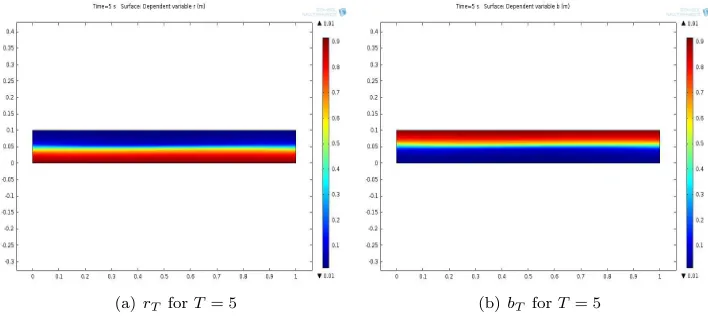
(a)rT forT = 5 (b)bT forT = 5

Fig. 3.ExampleII: Red and blue particle distribution at timeT= 5forming weak lanes.

(5.1)

r0(x, y) =cr+ 0.02 sin(πx) cos

πy

0.1

,

b0(x, y) =cb−0.02 sin(πx) cos

πy

0.1

with cr = cb = 0.4. Figure 2 illustrates the initial value r0 and the solution rT to system (3.1) at time T = 5, where it can be seen that in this setting the solution returns back to the equilibrium state quickly.

5.2. Example II: Lane formation. The behavior of solutions to system (2.7) corresponding to the scalingγ1−γ2=O(ε) is different. Settingγ0= 0.001,γ1= 0.5,

γ2 = 0.4,α= 0.2, and ε= 0.05 such that γ1−γ2 =δεfor δ= 2, and choosing the

same initial values (5.1) as above, we obtain the weak lane formation illustrated in Figure 3. Asγ1> γ2, the individuals have a tendency to step to the right. Therefore,

red individuals are highly concentrated on the bottom of the domain, whereas the blue individuals move to the top.

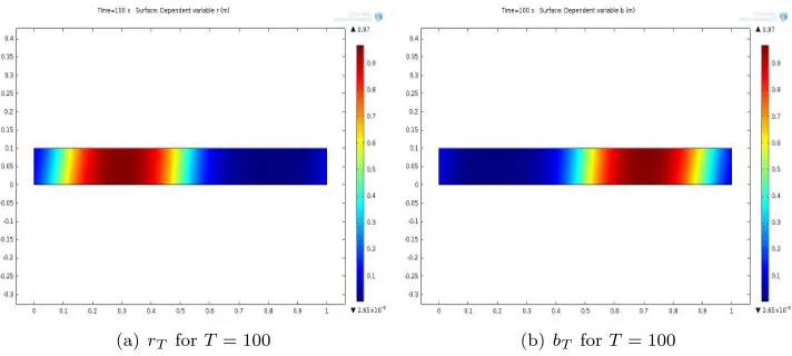
Figure 4 shows the cross section of the 2D solutionrT at timeT = 100 for different

0 0.01 0.02 0.03 0.04 0.05 0.06 0.07 0.08 0.09 0.1 0

0.1 0.2 0.3 0.4 0.5 0.6 0.7 0.8

y

r(y)

c=0.25,γ 0=0.0001 c=0.25,γ

0=0.001 c=0.1,γ₀=0.0001

c=0.1,γ₀=0.001

(a)rat timeT = 100

0 0.01 0.02 0.03 0.04 0.05 0.06 0.07 0.08 0.09 0.1 0

0.1 0.2 0.3 0.4 0.5 0.6 0.7 0.8

y

b

(y)

c=0.25,γ 0=0.0001

c=0.25,γ₀=0.001 c=0.1,γ

0=0.0001

c=0.1,γ 0=0.001

(b)bat timeT= 100

Fig. 4.ExampleII: Red and blue particle density in they-direction at timeT = 100.

0 0.01 0.02 0.03 0.04 0.05 0.06 0.07 0.08 0.09 0.1 0

0.1 0.2 0.3 0.4 0.5 0.6 0.7 0.8

y

f(y)

f(y)=r(y) f(y)=b(y) f(y)=ρ(y)

Fig. 5. Example II: Red and blue particle density as well as their sumρat timeT = 100in the case of nonequal initial mass.

(a)rT forT = 100 (b)bT forT = 100

Fig. 6. ExampleIII: Congestion in the red and blue particle density resulting in a deadlock.

initial masses. The parameters are the same as above, while the constantscr=cb=c in the initial values (5.1) are being varied. We observe that weak lane formation is more pronounced for smaller values of γ0 as well as higher densities. The transition

region aroundy= 0.05 decreases for smaller diffusitivity and greater mass, while the behavior ofris the same in the low-density region (0.05,0.1) for all parameter sets.

In the case of different masses Mr and Mb we observe asymmetric weak lane formation. We choose initial values of the form (5.1), i.e., cr = 0.4 and cb = 0.1. Figure 5 shows the formation of such weak lanes due to the side-stepping mechanism even though the massMb is smaller thanMr.

5.3. Example III: Jam. We conclude with a numerical simulation of the mini-mal model (3.1) showing another well-known phenomena in crowd dynamics, namely, traffic jams or so-called freezing. If the diffusion coefficients are small, i.e.,ε= 0.05 andγ0= 0.0001, it may happen that the individuals cannot move in their walking

rection any more as the initial masses are high compared to the diffusion coefficients. This ends in a jam or “frozen” configuration, as Figure 6 illustrates.

Acknowledgment. The authors would like to thank Christian Schmeiser for his helpful suggestions and discussions.

REFERENCES

[1] K. Anguige and C. Schmeiser,A one-dimensional model of cell diffusion and aggregation,

incorporating volume filling and cell-to-cell adhesion, J. Math. Biol., 58 (2009), pp. 395–

427.

[2] N. Bellomo and C. Dogbe, On the modeling of traffic and crowds: A survey of models,

speculations, and perspectives, SIAM Rev., 53 (2011), pp. 409–463.

[3] V. J. Blue and J. L. Adler,Cellular automata microsimulation for modeling bi-directional

pedestrian walkways, Transportation Res. B Methodological, 35 (2001), pp. 293–312.

[4] M. Burger, M. Di Francesco, J.-F. Pietschmann, and B. Schlake, Nonlinear

cross-diffusion with size exclusion, SIAM J. Math. Anal., 42 (2010), pp. 2842–2871, doi:10.

1137/100783674.

[5] M. Burger, M. D. Francesco, P. A. Markowich, and M.-T. Wolfram,Mean field games

with nonlinear mobilities in pedestrian dynamics, Discrete Contin. Dyn. Syst. Ser. B, 19

(2014), pp. 1311–1333, doi:10.3934/dcdsb.2014.19.1311.

[6] M. Burger, P. Markowich, and J.-F. Pietschmann,Continuous limit of a crowd motion

and herding model: Analysis and numerical simulations, Kinet. Relat. Models, 4 (2011),

pp. 1025–1047.

[7] M. Burger and J.-F. Pietschmann,Flow Characteristics in a Crowded Transport Model, preprint, arXiv:1502.02715, 2015.

[8] M. Chraibi, U. Kemloh, A. Schadschneider, and A. Seyfried,Force-based models of

pedes-trian dynamics, Netw. Heterog. Media, 6 (2011), pp. 425–442. doi:10.3934/nhm.2011.6.425.

[9] R. M. Colombo, M. Garavello, and M. L´ecureux-Mercier,A class of nonlocal models for

pedestrian traffic, Math. Models Methods Appl. Sci., 22 (2012).

[10] R. M. Colombo and M. D. Rosini,Pedestrian flows and non-classical shocks, Math. Methods Appl. Sci., 28 (2005), pp. 1553–1567.

[11] E. Cristiani, B. Piccoli, and A. Tosin,Multiscale modeling of granular flows with application

to crowd dynamics, Multiscale Model. Simul., 9 (2011), pp. 155–182.

[12] P. Degond, C. Appert-Rolland, J. Pettr, and G. Theraulaz,Vision-based macroscopic

pedestrian models, Kinet. Relat. Models, 6 (2013), pp. 809–839. doi:10.3934/krm.2013.6.

809.

[13] M. Dreher and A. J¨ungel,Compact families of piecewise constant functions inLp(0, t;b),

Nonlinear Anal., 75 (2012), pp. 3072–3077.

[14] M. Fornasier, B. Piccoli, and F. Rossi,Mean-field sparse optimal control, Philos. Trans. R. Soc. Lond. Ser. A Math. Phys. Eng. Sci., 372 (2014), doi:10.1098/rsta.2013.0400. [15] M. Fukui and Y. Ishibashi,Self-organized phase transitions in cellular automaton models for

pedestrians, J. Physical Soc. Japan, 68 (1999), pp. 2861–2863.

[16] G. Giacomini and J. Lebowitz,Exact macroscopic description of phase segregation in model

allows with long range interactions,I. Macroscopic limits, J. Stat. Phys, 87 (1998), pp. 37–

61.

[17] D. Helbing, I. Farkas, and T. Vicsek,Simulating dynamical features of escape panic, Nature, 407 (2000), pp. 487–490.

[18] D. Helbing and P. Molnar,Social force model for pedestrian dynamics, Phys. Rev. E, 51 (1995), p. 4282.

[19] S. Hittmeir and A. J¨ungel,Cross diffusion preventing blow-up in the two-dimensional

Keller-Segel model, SIAM J. Math. Anal., 43 (2011), pp. 997–1022, doi:10.1137/100813191.

[20] S. P. Hoogendoorn and P. H. Bovy,Pedestrian route-choice and activity scheduling theory

and models, Transportation Res. B Methodological, 38 (2004), pp. 169–190.

[21] R. L. Hughes,A continuum theory for the flow of pedestrians, Transportation Res. B Method-ological, 36 (2002), pp. 507–535.

[22] A. J¨ungel, The Boundedness-by-Entropy Principle for Cross-Diffusion Systems, preprint, arXiv:1403.5419, 2014.

[23] A. Kirchner and A. Schadschneider,Simulation of evacuation processes using a

bionics-inspired cellular automaton model for pedestrian dynamics, Phys. A, 312 (2002), pp. 260–

276.

[24] C. Koutschan, H. Ranetbauer, G. Regensburger, and M.-T. Wolfram,Symbolic

Deriva-tion of Mean-Field PDEs from Lattice-Based Models, preprint, arXiv:1506.08527, 2015.

[25] A. Lachapelle and M.-T. Wolfram,On a mean field game approach modeling congestion and

aversion in pedestrian crowds, Transportation Res. B Methodological, 45 (2011), pp. 1572–

1589.

[26] J.-M. Lasry and P.-L. Lions,Mean field games, Jpn. J. Math., 2 (2007), pp. 229–260. [27] B. Maury, A. Roudneff-Chupin, and F. Santambrogio,A macroscopic crowd motion model

of gradient flow type, Math. Models Methods Appl. Sci., 20 (2010), pp. 1787–1821.

[28] M. Moussaid, E. G. Guillot, M. Moreau, J. Fehrenbach, O. Chabiron, S. Lemercier, J. Pettr´e, C. Appert-Rolland, P. Degond, and G. Theraulaz,Traffic instabilities in

self-organized pedestrian crowds, PLoS Comput. Biol., 8 (2012), e1002442.

[29] B. Piccoli and A. Tosin,Pedestrian flows in bounded domains with obstacles, Contin. Mech.

Thermodyn., 21 (2009), pp. 85–107.

[30] B. A. Schlake,Mathematical Models for Particle Transport: Crowded Motion, Westf¨alische Wilhelms-Universit¨at M¨unster, 2011.

[31] N. Zamponi and A. J¨ungel,Analysis of Degenerate Cross-Diffusion Population Models with

Volume Filling, preprint, arXiv:1502.05617, 2015.