Marriage, Divorce, Remarriage: The Catalyst Effect of Unilateral Divorce

Munich Personal RePEc Archive

Marriage, Divorce, Remarriage: The

Catalyst Effect of Unilateral Divorce

Li, Li and Mak, Eric

Shanghai University of Finance and Economics, Shanghai University

of Finance and Economics

19 December 2016

Marriage, Divorce, Remarriage: The

Catalyst Effect of Unilateral Divorce

(Not for Public Circulation)

Eric Mak

, Li Li

Dec 19, 2016

Abstract

Unilateral divorce catalyzes the dissolution of unstable mar-riages and reorganizing better ones. To examine how unilat-eral divorce affects marital duration, we develop a simple DID stochastic dominance comparison across legal regimes and mar-ital cohorts. This DID comparison identifies that unilateral di-vorce catalyzes the dissolution of unstable marriages; more im-portantly, remarriages after the termination of first marriages also undergo significantly faster in the unilateral regime. We study the underlying mechanism using a parsimonious unitary model of marriage-remarriage cycle with three features: 1) on-the-job (marriage) search (OJS); 2) marital investment; 3) OJS feedbacks as an exogenous spousal separation event in the equi-librium. Under unilateral divorce, the lowered time cost involved in separation results in front-loaded OJS.

∗_{Shanghai University of Finance and Economics. Email: eric@mail.shufe.edu.cn.} †_{Shanghai University of Finance and Economics. Email: lili@mail.shufe.edu.cn.} ‡_{We thank Shouyong Shi, Randall Wright, Kenneth Burdett and Benoit Julien for}

1

Introduction

Rather than ”Till death do us part”, ”Marriage, Divorce, Remarriage” (Cherlin,2009) better describes American marriages since the later half of the 20th century — almost half of the modern American couples eventually divorce, yet more than half of the divorcees remarry within a few years. In the formation of this modern marriage cycle, the divorce rate rose by more than 200% during the 1970s.1 Concurrently, unilateral divorce was being introduced throughout the states; with divorces made easier, unilateral divorce was said to unintentionally caused the observed ”breakdown of American marriages and families” (Weitzman, 1985).

Weitzman’s critique was influential within academia, drawing the attention of many family researchers discussing its empirical validity (Peters,1986, 1992;Allen,1992; Friedberg, 1998;Wolfers,2006); it is also found that unilateral divorce significantly hurt the welfare of children whose parents experienced divorce (Gruber,2004). While in sharp contrast, policy-makers have never treated unilateral divorce as a Pandora’s Box — the rollout of unilateral divorce has faced no serious opposition, and that no states have ever turned back to the consensus regime.2 As we argue, this smooth policy rollout could be due to a pro-unilateral divorce argument: Unilateral divorce catalyzes the dissolution of undesirable marriages, allowing suffering couples to separate earlier; after divorce, the involved parties can form a better remarriage. Hence, rather than just breaking down marriages, unilateral divorce reconstructs them.

Given this background, we examine whether unilateral divorce catalyzes the marriage life-cycle `a laCherlin(2009); and if so, how. To this end, we quantify how unilateral divorce affects both the duration of the first marriage and the time to the second marriage since first marriage termination. As a study of divorce timing, our primary statis-tic of concern is the marital duration condition on eventual divorces.

1_{See Figure 1 inGruber(2004).}

2_{The transition to unilateral divorce is now complete, with New York being the}

This focus sets this paper apart from the previous empirical literature on unilateral divorce, that concerns the divorce rate instead.3

For identification, we need to control for common time trend and static differences in marital durations across states. So we de-velop a simple extension of stochastic dominance comparison as a difference-in-difference design (DID), and apply it with respect to legal regime and marital cohort. Like the standard DID, this method can be expressed as a regression. Hence controlling for observables is straightforward.

Using this research design, we find that unilateral divorce disso-lutes unstable marriages: Among relatively unstable marriages with duration less than or equal to 10 years, being the unilateral regime shortens the average marital duration by 0.7 years; the remaining mar-riages are more stable through selection, such that among marmar-riages that have a duration exceeding 10 years, their average duration is lengthened. Whereas after the termination of the first marriage, the unilateral regime has a 10% larger remarriage probability within 3 years relative to the consensus regime — a surprising result if unilat-eral divorce mechanically shortens the divorce process; whereas this finding is consistent with a hypothesis that, before the termination of the first marriage, divorcees in the unilateral regime tend to begin searching for new mates already.

To explain this catalyst effect, we appeal to the seminal work of

Becker et al. (1977), which proposes that marriages can dissolute due to either exogenous shocks and the arrival of a superior on-the-marriage (job) offer (hereafter OJS). We construct a dynamic model of marriage with both mechanisms as two sides of the same coin — within a couple, OJS reciprocally feedbacks as an exogeneous shock for the other spouse. As such, this model captures both the catalyst effect — the married continue to search for better opportunities— as well as Weitzman (1985)’s concern that some of the divorces could be involuntary. As one notable feature of our model, divorce takes time to complete in both regimes, and ends faster in the unilateral

3_{Some other papers examine marital durations as well, although their focuses}

regime; in a standard OJS model, an accepted OJS offer immediately take effect.

In the model, a representative agent voluntarily decides to marry when an offer arrives. During marriage, the representative agent can engage in marital investment (Stevenson, 2007; Voena,2015) and also engage in OJS. Due to either OJS or exogeneous separation, eventually the representative agent must divorce and restart the marriage cycle. Tracking the locus of the representative agent results in a steady state distribution of marriage duration. Because marriage quality tends increase over time due to marital investment, OJS becomes less attractive over time. As a result, OJS in this model exhibits negative duration dependence.

To clarify our main point —the interaction between OJS and mar-ital investment— our model abstracts away many realistic features, including age, learning, ex-ante heterogeneity, childbearing, cost of marriage, and legal costs of divorce.4 Also, we limit ourselves to a one-sided model instead of modelling the interaction between two spouses.

Despite the simplicity, this barebone model can already match, to a first order, both the marriage and divorce rates, as well as the duration of marriages and time required to have the next marriage in the United States. To mimic the effect of unilateral divorce, we consider a comparative static exercise of reducing the length of divorce. There are several effects. First, it increases the option value of a successful OJS. Second, it increases the separation due to the equilibrium feedback mechanism. Third, marital investment decreases due to the reduced value of marriage. Given these effects, a simulation shows that OJS is only about 2% among all divorces in the consensus regime, while the figure rises to about 6% in the unilateral regime. The net welfare, however, increases by about 10% by switching to the unilateral regime.

4_{A couple of other papers study the dynamics of marriage and divorce.}

Thus this model is capable in handling all these issues —both positive and negative— that has been separately discussed in the previous literature on unilateral divorce. In a more elaborate version of this model, we also consider a more realistic case in which OJS offers have a possibility to expire; it helps explaining the differences between the two legal regimes.

We own our intellectual debt to two papers. Shi(2016) considers the first model that combines endogenous job upgrading and on-the-job search. His model about the labor market explains tenure effects on wage, the dispersion of wage among ex-ante homogeneous workers, and also front-loaded OJS. Taking an analogy to the marriage market, we borrow his idea to generate a non-degenerate marital duration distribution, and that OJS is front-loaded in the marriage cycle.5

The second paper that inspires our work is Burdett et al. (2004). That paper builds a model of marriage, in which either or both spouse can engage in search. If one spouse decides to search, the marriage become less stable. This makes the choice of staying in marriage being less attractive, which in turn justify search as the optimal choice. As a result, excessive turnover can occur among the multiple equilibria. While we opt for a simpler unitary setup, we capture the same feature using the equilibrium feedback of OJS.

2

Background

2.1

Unilateral Divorce and OJS

Historically, divorce in the United States could only happen if either spouse have a fault. Otherwise, divorce was forbidden by law even with mutual consent between the spouses. Known as the adversary system, a divorcing couple would need to present evidence of fault to either spouse to the court, with adultery and physical abuse being the leading legal grounds. This requirement induced a large number

5_{Because in the labor market OJS is usually directed, with workers and vacancies}

of false testimonies among those couples who had mutual consent to divorce (Wright Jr and Stetson,1978;Rheinstein,1971;Marvell,1989;

Friedman,2004).

As discussed inGruber(2004), in the 1950s a legal reform permits divorces in the absence of faults in the presence of mutual consent between the spouses; yet still, without in the cases without legal con-sent, proving faults is necessary. In the 1970-80s, California lawmakers removed the need for spousal consent in filing no-fault divorce, thus effectively making divorce unilateral. This practice is soon followed by a number of other states within the 10-year period, while the rest defer the switch to the unilateral regime until much later. The simulta-neous existence of unilateral and consensus states permit a cross-state comparison between the two legal regimes, thereby identifying the effects of unilateral divorce.

From a theoretical standpoint, unilateral divorce has been regarded as neutral to divorce (Peters, 1986). In the unilateral regime, a married person, being mistreated by his/her spouse, can now make a credi-ble threat of leaving the household. Though in a transferacredi-ble utility framework, the Coase theorem applies — these husbands would ade-quately compensate their wives, and divorce will not happen unless the outside option exceeds the total value of the original marriage (Becker et al., 1977). So as long as unilateral divorce does not gen-erate extra outside options, neutrality holds. In this regard, most exogenous shocks considered in the literature — loss in income, job displacment, disability, well-being shocks (Weiss, 1997;Charles and Stephens, 2004; Chiappori et al., 2016) — are not directly correlated to the legal regime.6 While in our model, unilateral divorce reduces the duration of the divorce process, thus increasing the value of OJS as an outside option. Consequently, unilateral divorce is non-neutral on divorce.

As an important remark, OJS can be related to having extramarital

6_{Weiss(1997) study how unexpected changes in income affects divorce, while}

affairs, but the two are conceptually distinct. Fair(1978) considers a theory of extra-marital affairs in which an economic agent decides how to spend the time between his/her spouse and his/her paramour — the context is one that the economic agent maintains a simultaneous relationship between the two. Consequently, optimality inFair(1978) is an interior solution which equalizes the marginal utilities from engaging in the two activities. Whereas in our model, a successful OJS —whose value is greater than that of the current marriage— would

lead to divorce of the current marriage.

2.2

Marital Investment

Marital investment in this model is also endogenous. Stevenson(2007) provides empirical evidence on how unilateral divorce reduces marital-specific investments. For instance, the paper reports that couples in the unilateral regime are ”10% less likely to be supporting a spouse through school. They are 8% more likely to have both spouses em-ployed in the labor force full time and are 5% more likely to have a wife in the labor force. Finally, they are about 6% less likely to have a child.” In our model, Foreseeing that the marriage may end early due to OJS, it becomes harder to reap the benefit of marital upgrading. Consequently, couples in the unilateral regime would react by choos-ing less marital investment. Our model formalizes the essence of her argument.

Related, Voena(2015) argues that property division under unilat-eral divorce matters. Some states divide the joint assets equally or based on equity, while the others states sort to the pre-marriage legal ownwership of each asset. Due to these legal restrictions, utility is not perfectly transferable, and hence unilateral divorce may have varied impact on investment within the household.

3

Empirical Strategy

As suggestive evidence, we first examine a plot of the cumulative density function of marriage duration in Figure1, reproduced from a seminal review (Stevenson and Wolfers,2007). During the unilateral divorce reform that largely happened in the 1970s, the 1950-59 marital cohort has already passed its early years of marriage, so that it is not affected by the catalyst effect of unilateral divorce; the reverse is true for the 1970-79 marital cohort.7 Hence by comparing these two marital cohorts, we can obtain a sense of how the catalyst works. For the 1950-59 marital cohort, among the eventual divorces in a 15 year window, about half of them happened within the first 6 years; the corresponding proportion rises to about two thirds for the 1970-79 marital cohort. As such, eventual divorces happened earlier for the 1970-79 marital cohort relative to the 1950-59 cohort, i.e. the marital duration distribution becomes more front-loaded over time.

Nevertheless, Figure1pools all states together regardless of their legal regime, and that it is clear that marriages have strong cohort effects undermine the identification of a catalyst effect from unilateral divorce. The empirical literature already found unilateral divorce has little long-run effect on the divorce rate (Wolfers,2006), despite that the large concurrent increase in divorce rate; there is no reason to believe that the cohort effects for marital duration are small. As documented by Cherlin (2009) and Stevenson and Wolfers (2007), cohort effects are due to many reasons such as changes in culture, wage structures, introduction of new household technologies.

To address this issue, we distinguish the states by both cohort and legal regime, studying marital duration using a difference-in-difference (DID) identification strategy. We assume that between the treated states (switchers during 1970-79) and the control states (non-switchers during 1970-79), their cohort effects —the changes between 1950-59 to 1970-79— are common. A DID estimator eliminates this common cohort effect and also the fixed heterogeneity in marital duration between states.

7_{A marital cohort is defined as the subset of respondents in the data who are}

3.1

Sample Selection, Right Censoring, and Legal Regime

Definitions

This paper uses the data from the Survey of Income and Program Participation (SIPP) 2001. While the SIPP is mainly used for the study of income and labor force related issues, the data set also contains a topical module that retrospectively inquires the marital histories of the survey respondents. Notably, this topical module contains their exact years of first and second marriages, separation and termination, if applicable. The topical module also contains some geographic and contextual variables such as race, gender and education which allows us to condition our results on them.

The SIPP is repeated annually, and we select the 2001 SIPP for two reasons. One reason is that in 2001, the median respondents are in their mid-30s. Many of them were just married during the 1980s, after the unilateral divorce movement has mostly ended. The second reason is that this data set since this is used inStevenson and Wolfers(2007) as well, and hence we adopt it for consistency.

Regarding sample selection, we consider only the respondents who have had their first marriages, and we select the 1950-59 marital cohort and the 1970-79 marital cohort. We then select a subset of respondents that reside in a set of states that has a clear coding of the year of switching to the unilateral regime. Some respondents do not reside in the United States, and we exclude them in the analysis.

To provide an idea of the sample selection process, we report the sample selection statistics in Table 1. The table reveals that there is substantial right-censoring: since the survey is taken in the year of 2001, marriages that do not end by 2001 does not reveal its duration in the data. In our sample, about half of the duration observations are censored. The significant right-censoring forbids us to reliably infer the whole uncensored duration distribution or its summary statistics such as the median or mean. Consequently, we do not attempt to estimate parametric duration models of marriage as inLillard(1993) or Georgellis (1996). Instead, we compare only the left tail of the duration distribution across legal regimes and marital cohort, which is free from the right-censoring problem.

The regime coding used in this paper follows that in Friedberg

asStevenson and Wolfers (2006). It should be noted there are some minor discrepancies between the exact year of regime switching used by different authors, due to the fact that the exact terms of unilateral divorce are heterogeneous. However, in this paper, our identification strategy does not exploit information on the exact year of regime change, thus being free of this definitional issue. We define a dummy variable “Uni1980” which is 1 if the state is in the unilateral regime on or before 1980, and 0 otherwise.

3.2

Difference-in-Difference Plots

Let c ∈ {0, 1} denote the cohort (0 for the 1950-59 cohort, 1 for the 1970-79 cohort). Lets ∈ {0, 1} denote the legal regime as in the year 1980: that is,s =0 for the states which remain in the consensus regime by 1980,s=1 for the states which switched to the unilateral regime on or before 1980.

The 1950-59 marital cohort did not experience unilateral divorce reform in the 1970-80 within their first 10 years of marriage. For the 1970-79 marital cohort, the respondents in the unilateral regime are affected but those in the consensus regime are unaffected. This observation allows us to construct the following DID estimate with respect to the expected duration:

D= (E[X|c=1,s=1,X ≤x]¯ −E[X|c =1,s =0,X ≤x])¯ −(E[X|c=1,s=1,X ≤x]¯ −E[X|c =0,s =0,X ≤x])¯ (1)

whereX is the duration, a random variable censored to be less than a duration threshold ¯x ∈ R_{+. Since we are focusing on unstable}

marriage in this paper, ¯x=10 unless otherwise specified.

Next we show that this DID strategy identifies a front-loading effect. Front-loading of a distribution refers to a left shift in mass for a duration distribution with a fixed support. Formally, we define front-loading by second-order stochastic dominance of the cumulative density functions (cdfs hereafter):

Definition 1 (Front-Loading). Between two distributions A and B with the same bounded support X ≡ [0, ¯x] and cdfs FA,FB : X → [0, 1], one

distribution is more front-loading if 1_x¯ R₀x¯FA(x)dx > 1_x¯

Rx¯

that on average, the cdf of A is greater than the cdf of B at any duration x ∈ X.

The idea behind this definition is that if the value of cdf of one distribution is on average larger than that of the other distribution, then the first distribution has relative more respondents having small marital durations.

This definition requires the two distributions to have a common bounded support. For labor market context, the support of the work duration (tenure) distribution is naturally defined as the time interval between labor market entry and the retirement age, 60-65 in most countries, and that it is typically policy-variant. Consequently, the discussion of whether OJS is front-loaded in the labor market context is unambiguous. Whereas for a marriage, there is no parallel definition to retirement age — marriages end idiosyncratically either by divorce or death of a spouse. To define the support for marriage duration, we impose a censoring rule by focusing only on the marriages that end in divorce within a fixed duration threshold, denoted by ¯x. This duration threshold in our main specification is set to be 10 years, since we focus on the unstable marriages.

Next we show that our DID estimate corresponds our front-loading definition.

Proposition 1. Let Fcs(x) = Pr(X|C = c,S = s,X ≤ x). The DID

estimate can be reexpressed as:

D=

Z _x¯

0 [(F10(x)−F11(x))−(F00(x)−F01(x))]dx (2)

The proof of Proposition1direct follows from integration by parts. According to this result, the DID estimate evaluates how the unilateral distribution is front-loaded relative to the consensus distribution for the 1970-79 cohort, and then compare this front-loading measure against the counterpart of the 1950-59 cohort. Unilateral divorce has a front-loading effect ifD <0 (notice the reversal in sign).

representing the unilateral and consensus regime respectively. For each marital cohort and at each given duration, the unilateral regime has a higher cumulative divorce probability than the consensus regime. Across marital cohorts, there is a large increase in cumulative divorce probability for both regimes. However, the increase is heterogeneous across the two regimes: for the 1950-59 cohort, the two series diverge with respect to marital duration, while the 1970-79 cohort does not show convergence.

After censoring, we plot Figure4to show the graph of the function

d, defined by:

d(x) ≡10∗[(F₁₀(x)−F₁₁(x))−(F00(x)−F01(x))]

which is the integrand in Equation 2 multiplied by ¯x = 10. As illustrated by the derivations above, its average over the support Y ≡ [0, 10] is the DID estimate. A negative value indicates a front-loading effect.

We then study whether the catalyst effect in the unilateral regime cleanse out the unstable marriages, leaving only the stable marriages by selection. Figure5shows a similar graph with the threshold set at

¯

x =20. The graphs of dhas a large jump from being negative to being positive at around x =10, which indicates that unilateral divorce has more stable long-run marriages than consensus regime, after netting cohort and state effects.

Finally, we study remarriages. Among the respondents who marry twice or more, we evaluate the duration to second marriage for ac-cording to the following definition:

Duration to Second Marriage_i =

Year of Second Marriage_i−Year of First Termination_i (3)

4

Regressions

4.1

First Marital Duration

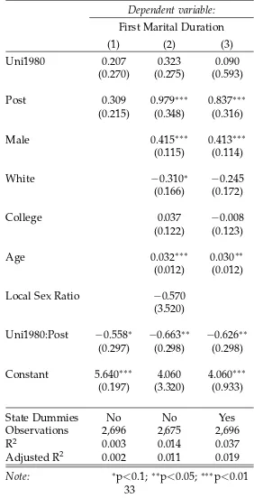
The DID analysis can be straightforwardly extended to include co-variates. Table2 reports the OLS estimates of a set of individual-level regressions. The dependent variable is first marital duration; we run this regression with a subsample whose first marital duration is less than or equal to 10 years. Column 1 is the base regression with ”Uni1980” being the legal regime dummy, 1 if the state becomes unilateral by the year of 1980. Post is a cohort dummy which is 1 if the individual belongs to the 1970-79 marital cohort, 0 if he/she belongs to the 1950-59 marital cohort. The specification of this base regression is:

First Marital Durationi =

β0+β1Uni1980i+β2Posti+β3Uni1980i∗Posti+εi (4)

Standard arguments imply that our parameter of interest, β3,

cor-responds to our previous DID estimate; while β1,β2 capture fixed

the specification becomes:

First Marital Durationi=

β0+

S

∑

s=1

d_si+β2Posti+β3Uni1980i∗Posti+Xiβ+εi (5)

whered_si =1 if the respondentiresides in state s, 0 otherwise; X_i are a vector of individual-level covariates.

These specifications provide similar estimates of the effect of uni-lateral divorce on expected marital duration of about −0.6 (in years). These figures are consistent with the magnitudes identified from from the previous DID graphs. While slightly more than half a year may appear to be small relative to the entire marital distribution with duration less than or equal to 10 years, it should be noted that the marital duration distribution is rather stable across groups defined by observables, unlike marriage and divorce rates. In particular, the standard deviation of mean marital duration across states are only 1.54 years and 1.2 years for the 1950-59 and 1970-79 cohorts respectively, so that our estimates are moderately large.

We then consider heterogeneous treatment effects. Table3reports the estimates by gender, race, and education. We find that the treat-ment effects are large for females, non-white, and those without a college degree — for non-whites, the estimate is particularly large, with a value of -1.724 years. While the effects for males, white, and col-lege graduates are smaller and mostly statistically insignificant from zero. This finding is consistent with a hypothesis that disadvantaged groups are more likely to benefit from unilateral divorce.

4.2

Remarriage

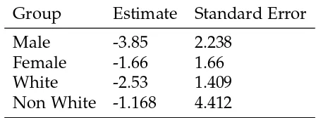
We find that adding individual-level covariates and state-level dummies increases the DID estimate, such that Column 3 reports an estimate of -2.650 (in years), which is more than half of the duration of 5 years within our selected sample. We then show the heterogeneous treatment effects in Table5. We find the opposite result of Table3: the catalyst effect of unilateral divorce for remarriage is stronger for males and whites. Note that because remarriage involves a smaller sam-ple (only those who terminates the first marriage and the remarried within 5 years are included), and that the college graduates is a small portion of the total population, we are unable to reliably estimate a heterogeneous treatment effect model with respect to education.

4.3

Robustness

Our DID strategy relies on a common trend assumption. To check this assumption, we consider a placebo DID using the 1940-49 and 1950-59 cohorts. Neither of the cohorts experienced unilateral divorce in their first 10 years of marriage, thus we expect to find a zero effect. We perform the same DID analysis and find no effects on both first marriage duration and remarriage.

5

Model

5.1

Setup

As a conceptual exercise, this section builds a model to capture the dynamics of marriage, divorce, and remarriage. We consider a con-tinuum of agents which are homogeneous before marriage. Time is continuous. The discount rate isr ∈ [0, 1]. Each marriage is character-ized by its marriage capitaly ∈ Y ≡[0, ¯y] which is fully specific to the marriage. For a person in the divorce process, we denote his OJS offer also byy∈ Y if present; if the divorce has no accompanying OJS offer, we use a notation∅ _{to denote the state.}

An agent at any instant is in one of four population pools: married

M, divorcing with OJS offer D, divorcing without OJS offer ∅_{, and}

flowchart (Figure7). We describe the actions and events at each node of the flowchart in detail below.

For simplicity, we do not model the contact between opposite sexes explicitly. Instead, a successful search of an agent leads she to a pool of ”reserves” —a mass of the opposite sex who are willing to form a match if she agrees— and that the matched output belongs solely to the agent; alternatively, the output is interpreted as the agent’s share of output under a fixed sharing rule. A full, two-sided extension is left for future research.

5.2

Actions, Events, and Values

5.2.1 Married Agents

An agent in the married pool M is in a marriage. For an agent with marriage capital y, he involves in two possible actions, namely OJS and upgrading.

1. The first action is OJS. He controls the OJS arrival rate λ ∈ R₊

at a cost cλ(λ). A successful OJS is characterized by a potential marriage quality x ∈ Y, drawn from a quality distribution with cumulative density function is F : R_{+ → [0, 1]. If successful,}

then the agent enters the divorce process with the OJS offer x.

2. The second action is to upgrade the existing marriage, which stands for marital investment. We model upgrading stochas-tically with arrival rate φ ∈ R_{+, to be chosen by the agent at}

a cost cφ(φ). When upgrading arrives, the marriage capital y increases to a level G(y) ∈ [y, ¯y]and the marriage is maintained. The functionG : Y → Y is strictly increasing.

The two costs functions cλ,cφ : R+ →R+ are both strictly increasing and convex, and satisfy Inada conditions.

In the equilibrium, successful OJS by spouse feedbacks as part of the exogeneous separation rate, with an arrival rate

s∗(y) = s¯+λ∗(y)

where ¯s∈ R_{+is a base separation rate, andλ}∗_{(y)is the policy function}

does not take into account hows∗(y) changes withλ∗(y), but rather taking it as given.

The flow value for a married agent with marriage capital yis the sum of several components. The first is the flow output generated by the marriage capitalQ(y), whereQ : Y →R_{+is strictly increasing and}

twice differentiable. The second is the OJS component: after paying an OJS cost ofcλ(λ), with arrival rateλthe agent freely chooses between an OJS offer and keeping the present marriage; in case he accepts the OJS offer of qualityx, he enters the divorce pool with a value gain of

V_D(x)−V_M(y). The third is the upgrading component: after paying an upgrading cost ofcφ(φ), with arrival rate φthere is a gain in value

VM(G(y))−VM(y). The fourth is exogenous separation, in which with

arrival rates∗(y) there is a value gain ofV∅−V_M(y). Summarizing

the above, we have the following epression:

rVM(y) = max

λ,φ∈R₊Q(y) +λ

Z

Y max{VD(x)−VM(y), 0}dF(x)−cλ(λ)

+φ[VM(G(y))−VM(y)]

+s∗(y)[V∅−VM(y)] (6)

5.2.2 Divorcing Agents

We shut down legal costs of divorce, so divorcing receives zero flow payoff. The divorce process terminates with rateθD ∈ R+. A divorcing

agent with an OJS offer becomes married with the OJS offer being realized.8

As such, the flow value for an agent in the divorce process is given by:

rVD(y) =θD[VM(y)−VD(y)] (7)

A divorcing agent without an OJS offer (due to exogenous separa-tion) becomes single after the divorce process is terminated. Therefore,

rV∅ =θD[VS−V∅] (8)

8_{It is easy to generalize this model to consider the possibility of losing the OJS}

In a more elaborate version of this model, we also consider a more realistic case in which OJS offers have a possibility to expire — it can be difficult to have the potential partner to wait for many years until the current marriage is dissoluted. If this is the case, then the Bellman equation ofVD(y)would involve an extra term that governs

the rate of losing the OJS offer, entering the group of divorcing agents without OJS offer V∅. Thus on top of pure time cost, this feature

helps explaining the differences between the consensus and unilateral regime.

5.2.3 Available Agents

Being available receives zero flow payoff, and with arrival rateθ_S→M :∈

R_{+ the agent receives an offer to marry — with probability another}

available individual, and decides whether to enter a marriage. In principle, the potential spouse could be also available, or she could be from OJS. Consequently, the flow value of being single is given by:

rVA =θA→M

Z

Ymax{VM(x)−VA, 0}dF(x) (9)

5.3

Characterizations

Proposition 2(OJS Arrival). λ∗(y)is decreasing in y.

Proof. The first-order condition for λis: Z

Ymax{VD(x)−VM(y), 0}dF(x) =c ′

λ(λ)

Since V_M′ (.) < 0, LHS is strictly decreasing in y. Since c_λ(.) is

strictly convex, the OJS policyλ∗(y)is strictly decreasing iny. Whereas the first-order condition for upgrading is:

V_M(G(y))−V_M(y) = c′_φ(φ)

The presumption that V_M′ (.) > 0 and the Inada condition jointly

imply that φ∗(y) > 0, such that positive upgrading exists in the

OJS among married agents follows a reservation policy, such that OJS is taken if the drawn offer is better than than the reservation value

R(y). Define the reservation value RM(y) by:

V_D(R_M(y)) = V_M(y)

Proposition 3(Increasing Reservation Value for OJS). RM(y) is strictly

increasing in y, such that the reservation value of OJS increases with marriage capital.

Proof. The envelope condition forVD(y)is:

rV_D′ (y) =θD[VM′ (y)−VD′(y)]

which implies that for ally:

V_D′(y) = θD r+θD

V_M′ (y) >0

Differentiating the reservation value condition for OJS, we have:

R′_M(y) = V

′

M(y)

V_D′ (R_M(y)) >0

Together, the two propositions imply that both the endogenous OJS arrival rate and acceptance rate strictly decrease when marriage capital

y increases. This is because when the marriage capital is relatively high, OJS becomes harder to be successful, which in turn reduces the incentive to attempt on it. These two effects reinforce each other.

Rearranging (7) yields:

VD(y) = θD

V_M(y)

r+θD (10)

Notice that if θD → ∞, such that the divorce process

instanta-neously ends by realizing the OJS as a new marriage, thenV_D(y) = VM(y) for all y and that R(y) = y for all y is a solution of the

wage is just the current wage. Now because θD/(r+θD)∈ (0, 1), the

reservation value for OJS is higher than that of the standard case. Let R∗ ∈ Y be the reservation value of singles, defined by

V_A =V_M(R∗) (11)

Proposition 4 (Reservation Value for Singles). Suppose that θ_A→M is

sufficiently large. Then the reservation value of singles is strictly positive, such that R∗ >0.

Proof. We have:

rVS =θA→M

Z _y¯

R∗[VM(x)−VA]dF(x)

Suppose that R∗ = 0, which requires that V_A ≤ V_M(0). This implies that:

V_A = θA→M r+θA→M

Z

YVM(x)dF(x) When θA→M → ∞, VA →

R

YVM(x)dF(x) > VM(0), resulting in a contradiction.

Proposition4implies that when being married is sufficiently easy, the availables will wait until receiving a reasonably good match, re-jecting some of the received offers.

Proposition 5(Value after Exogeneous Separation). V∅ <V_A.

Proof. The proof is direct: V∅ = _r+θD_θ DVA

< V_A since _θD,r > 0 and

VS >0 by Proposition4.

Finally, we go back to prove that the value functions are strictly increasing.

Proposition 6(Increasing Value Function for Married and Divorcing). V_M′ (y),V_D′(y) >0for all y ∈ Y.

Proof. The envelope condition forV_M(y) is:

rV_M′ (y) = Q′(y) +λ∗(y){ Z ∞

R(y)[−V ′

−[VD(R(y))−VM(y)]f(R(y))R′(y)}

+φ∗(y)[V_M′ (G(y))G′(y)−V_M′ (y)]

+ds

∗_(y)

dy [VD(0)−VM(y)]−s

∗_(y)V′

M(y)

which simplifies to:

[r+λ∗(y)[1−F(R(y))] +φ∗(y) +δ+s∗(y)]V_M′ (y)

=Q′(y) +φ∗(y)V_M′ (G(y))G′(y)

+ds

∗_(y)

dy [VD(0)−VM(y)]

Suppose thatV_M′ (y) <0. Then LHS is strictly negtative.

Since there is no benefit in upgrading the marriage, we have φ∗(y) = 0. This presumption would also imply that OJS is strictly increasing in y and ds∗(y)/dy ≥ 0 as a result. Since V_D′(y),V_M′ (y)

have the same sign, we have VD(0)−VM(y) > 0. Also Q′(y) > 0.

Therefore, the RHS is strictly positive. So we have a contradiction.

5.4

Simulation

5.4.1 The Baseline

This subsection simulates a baseline model. The purpose of this simu-lation is to illustrate the basic cost and benefit calculus of marriages and divorce. The objective of this exercise is to check if it agrees with the marriage cycle desribed inCherlin(2009) to a first order in terms of both stock and flows.

We discretize both the space and time for the simulation. Spatially, we discretize the domain of marriage capital by introducing a 100-point grid. Temporally, we discretize the continuous time finely enough to guarantee that the events (OJS, upgrading, exogenous separation) do not simulataneously happen within one simulation period.9

We set the base separation rate to be ¯s=0.1. Given our chosen time scale of 1/10, this rate corresponds to a 0.1% per-period probability.

9_{In continuous time, it is not possible to have multiple events with independent}

The mean duration until first arrival is 100 periods or 10 years — we consider it a reasonable value to capture dissolution of marriages due to background events. We set θD = 0.5. Following the same

calculations, this implies that divorce takes an average of 2 years in the consensus regime, which is probably a slight underestimation of the truth. We set the arrival rate of offers for availables asθA→M =0.25,

which implies an average duration of 4 years to have a new potential mate to marry. The interest rate r is set to be 0.05, following the standard.

For the baseline without OJS and marriage upgrading, we use the following functional forms:

Q(y) = y+50

F(y) = 1/100

cλ(λ) =1000λ2

cφ(φ) =100φ2

G(y) = min{100,y+1}

The linear functional form of Q(y) is assumed for simplicity, with the slope is standardized to 1 by fixing the unit of marriage quality

y. Due to this standardization, values functions can be interpreted in terms of (present-value) units of output. The intercept, capturing the base preference of being married, is the only free parameter used in adjusting the simulation; the results are not very sensitive to this choice. The coefficients of the cost functions are set such that the equilibriumλ andφare comparable in magnitude to the exogenous separation rate ¯s.

The model is solved by value function iteration. Taking the avail-ables for instance, we rearrange (9) and establish an iteration as fol-lows:

V_Aj = θA→M r+θA→M

Z

Ymax{V

j−1

M (x),V j−1

A }dF(x) (12)

Figure8plots the value functions of the baseline case. The figure shows that the value of married is higher than the value of divorce for each level of marriage capital, which suggests thatR(y) <y. The

agent would require the OJS offer to be strictly higher in quality than the current marriage in order to accept it, because waiting for the divorce process to complete is costly.

5.5

Simulation

After numerically solving this model, we then simulate it for 1000000 periods to obtain a history of marital states and marriage capital. We start the baseline simulation (for consensus regime) with the agent being in the single state. Due to the long simulation, this choice is irrelevant to our results below. Then we simulate the model with θD =5, being 10 times as the baseline, to mimic the effect of unilateral

divorce. The corresponding duration of the divorce process reduces from 2 years to 0.2 years.

For the consensus regime baseline, the resulting marital duration distribution has a median of about 6 years, which is close to the his-torical average median marriage duration in the United States during 1867-1967 (Plateris,1973). After implementing unilateral divorce, the median marriage duration reduces to 5.1 years.

In the consensus regime, the ratio ofV∅/V_Ais 0.90, so that being

in the divorce process without an OJS offer is 10% worse than being single — the representative agent in the former state cannot begin searching for the next marriage. For the unilateral regime, the ratio becomes 0.9901, being very close to unity. This is because the waiting period disappears.

To evaluate welfare, for each regime we evaluate the average value along the simulation path. We then compute ratio between the average value in the consensus regime and that of the unilateral regime. We find a ratio of about 0.91, which suggests that although there are pros and cons of unilateral divorce (OJS and its reciprocal), the net welfare effect is positive.

In the consensus regime, the OJS population constitutes about 2% of all divorcing population. While in the unilateral regime, this percentage increases threehold to about 6%. The reason of this small number is that being married is voluntary. As long as marriage offers arrive sufficiently frequently, the representative agent would optimally choose to wait for a better offer. The reservation value would be relatively high, so that accepted marriages are generally of high quality. As a result, it would be difficult for a currently married individual to obtain an even better offer, especially after considering the time cost of being in the divorce process.

Figure9shows the endogenous OJS and upgrading arrival rates with respect to marriage quality, which are the policy functions. Con-sistent with our derivation, λ(y) is decreasing in y, while φ(y) is increasingyexcept at the upper boundary of the grid y=100, where upgrading is no longer possible.

Figure10 plots the histogram of simulated marriage quality. The fact thatλ(y)is decreasing in yindicates that this group of marriages are particularly unstable due to OJS, yet their dissolution is favorable because their value is much lower than that of being single. It also re-flects on the proportion of OJS among the divorcing individuals, which is about one-third; the remaining two-thrids are due to exogenous separation.

Figure11 plots the histogram of simulated marital duration. The model is able to generate a right-skewed distribution of marital dura-tion.

6

Conclusion

This paper presents some evidence on the effects of unilateral divorce on marriage duration, conditional on eventual divorce. We find that unilateral divorce indeed serves as a catalyst of divorce for the unstable marriages. Quoting fromStevenson and Wolfers(2007), there is a large sociology literature viewing marriage, divorce, and remarriage as a life-cycle. While certainly this cycle is not deterministic at the individual household level, this is not very far off as a general description.

marital cycle. In particular, for people who have divorced, they may have a distrust on the marital institution and decide not to remarry. Furthermore, since data on cohabitation is not as complete, and that considering it requires substantial treatment, we choose to leave this important issue to future work.

References

Allen, D. W. (1992): “Marriage and divorce: Comment,”The American

Economic Review, 82, 679–685.

Becker, G. S., E. M. Landes,andR. T. Michael(1977): “An economic

analysis of marital instability,”Journal of political Economy, 85, 1141– 1187.

Brien, M. J., L. A. Lillard, and S. Stern (2006): “Cohabitation,

marriage, and divorce in a model of match quality,” International Economic Review, 47, 451–494.

Bruze, G., M. Svarer,andY. Weiss(2014): “The dynamics of marriage

and divorce,”Journal of Labor Economics, 33, 123–170.

Burdett, K., I. Ryoichi,andR. Wright(2004): “Unstable

Relation-ships,”The BE Journal of Macroeconomics, 1, 1–44.

Charles, K. K.andM. Stephens, Jr(2004): “Job displacement,

dis-ability, and divorce,”Journal of Labor Economics, 22, 489–522.

Cherlin, A. (2009): Marriage, divorce, remarriage, Harvard University

Press.

Chiappori, P.-A., N. Radchenko, andB. Salanie´ (2016): “Divorce

and the duality of marital payoff,” Review of Economics of the House-hold, 1–26.

Choo, E. (2015): “Dynamic marriage matching: An empirical

frame-work,”Econometrica, 83, 1373–1423.

Choo, E.and A. Siow (2006): “Who marries whom and why,” Journal

Fair, R. C. (1978): “A theory of extramarital affairs,”Journal of Political

Economy, 86, 45–61.

Friedberg, L. (1998): “Did unilateral divorce raise divorce rates?

Evidence from panel data,” The American Economic Review, 88, 608.

Friedman, L. M. (2004): American Law in the twentieth century, Yale

University Press.

Georgellis, Y. (1996): “Duration of first marriage: does pre-marital

cohabition matter?” Applied Economics Letters, 3, 217–219.

Gruber, J. (2004): “Is making divorce easier bad for children? The

long-run implications of unilateral divorce,” Journal of Labor Economics, 22, 799–833.

Jacob, H. (1988): Silent revolution: The transformation of divorce law in

the United States, University of Chicago Press.

Jovanovic, B. (1979): “Job matching and the theory of turnover,”

Journal of political economy, 87, 972–990.

Lillard, L. A. (1993): “Simultaneous equations for hazards: Marriage

duration and fertility timing,”Journal of econometrics, 56, 189–217.

Marvell, T. B. (1989): “Divorce rates and the fault requirement,”Law

and Society Review, 543–567.

Peters, H. E. (1986): “Marriage and divorce: Informational constraints

and private contracting,” The American Economic Review, 76, 437–454.

——— (1992): “Marriage and divorce: Reply,”The American Economic Review, 82, 686–693.

Plateris, A. A. (1973): 100 Years of Marriage and Divorce Statistics,

United States, 1867-1967, National Center for Health Statistics.

Rheinstein, M. (1971): Marriage, Divorce, Stability and the Law,

Univer-sity of Chicago Press.

Shi, S. (2016): “Efficient Job Upgrading, Search on the Job and Output

Stevenson, B. (2007): “The impact of divorce laws on marriage-specific

capital,” Journal of Labor Economics, 25, 75–94.

Stevenson, B.and J. Wolfers (2006): “Bargaining in the shadow of

the law: Divorce laws and family distress,”The Quarterly Journal of Economics, 121, 267–288.

——— (2007): “Marriage and divorce: Changes and their driving forces,” The Journal of Economic Perspectives, 21, 27–52.

Voena, A. (2015): “Yours, Mine, and Ours: Do Divorce Laws Affect

the Intertemporal Behavior of Married Couples?” The American Economic Review, 105, 2295–2332.

Weiss, Y. (1997): “The formation and dissolution of families: Why

marry? Who marries whom? And what happens upon divorce,”

Handbook of population and family economics, 1, 81–123.

Weitzman, L. J. (1985): divorce revolution, Collier Macmillan.

Wolfers, J. (2006): “Did unilateral divorce laws raise divorce rates? A

reconciliation and new results,”The American Economic Review, 96, 1802–1820.

Wright Jr, G. C. and D. M. Stetson (1978): “The impact of

no-fault divorce law reform on divorce in American states,”Journal of Marriage and the Family, 575–580.

Figure 1: First Marriages Ending in Divorce, by Year of Marriage

Sample Size Uncensored #Obs Median Marriage Duration

Original Sample 72707

Married Sample 34338 14349 10

1950-59 Cohort (Unilateral States) 1755 886 18

1950-59 Cohort (Consensus States) 2326 1079 22

1970-79 Cohort (Unilateral States) 3155 1742 8

1970-79 Cohort (Consensus States) 3610 1853 9

Figure 3: Cumulative Divorce Probabilities by First Marital Duration

Table 2: OLS Regressions (First Marital Duration, Censored at 10 years)

Dependent variable:

First Marital Duration

(1) (2) (3)

Uni1980 0.207 0.323 0.090

(0.270) (0.275) (0.593)

Post 0.309 0.979∗∗∗ 0.837∗∗∗

(0.215) (0.348) (0.316)

Male 0.415∗∗∗ 0.413∗∗∗

(0.115) (0.114)

White −0.310∗ −0.245

(0.166) (0.172)

College 0.037 −0.008

(0.122) (0.123)

Age 0.032∗∗∗ 0.030∗∗

(0.012) (0.012)

Local Sex Ratio −0.570

(3.520)

Uni1980:Post −0.558∗ −0.663∗∗ −0.626∗∗

(0.297) (0.298) (0.298)

Constant 5.640∗∗∗ 4.060 4.060∗∗∗

(0.197) (3.320) (0.933)

State Dummies No No Yes

Observations 2,696 2,675 2,696

R2 0.003 0.014 0.037

Adjusted R2 0.002 0.011 0.019

Table 3: Heterogeneous Treatment Effect (Marital Duration)

Group Estimate Standard Error

Male 0.018 0.472

Female -1.042 0.392

White -0.305 0.323

Non White -1.724 0.781

College -0.509 0.621

Table 4: OLS Results (Remarriage): Censored at 5 years

Dependent variable:

Duration to Second Marriage

(1) (2) (3)

Uni1980 1.950∗ 2.220∗ 2.600

(1.150) (1.150) (2.750)

Post −2.840∗∗∗ −1.470 −0.321

(0.927) (1.630) (1.560)

Male 0.122 0.067

(0.544) (0.555)

White −0.336 0.008

(0.886) (0.925)

College −1.450∗∗ −1.530∗∗

(0.577) (0.597)

Age 0.070 0.087

(0.063) (0.065)

Local Sex Ratio 14.400

(16.200)

Uni1980:Post −1.890 −2.350∗ −2.650∗∗

(1.290) (1.280) (1.310)

Constant 11.500∗∗∗ −6.070 5.460

(0.825) (15.300) (4.750)

State Dummies No No Yes

Observations 1,015 1,011 1,015

R2 0.036 0.042 0.091

Adjusted R2 0.034 0.035 0.043

Table 5: Heterogeneous Treatment Effect (Duration to Second Mar-riage)

Group Estimate Standard Error

Male -3.85 2.238

Female -1.66 1.66

White -2.53 1.409

Single Married Divorcing with OJS

Divorce without OJS

matching

Exo. Separation OJS upgrading

remarry

Completing Divorce Process

200 300 400 500 600

0 25 50 75 100

y

value

variable

VM

VD

Vempty

VS

0.00 0.02 0.04 0.06 0.08

0 25 50 75 100

y

Arr

iv

al Rate

variable

lambda

phi

0 10000 20000

0 25 50 75 100

Marriage Capital

count

0 200 400 600

0 20 40 60 80

Marriage Duration

count