Does Oil Predict Gold? A Nonparametric Causality in Quantiles Approach

Munich Personal RePEc Archive

Does Oil Predict Gold? A

Nonparametric Causality-in-Quantiles

Approach

Shahbaz, Muhammad and Balcilar, Mehmet and Ozdemir,

Zeynel Abidin

Montpellier Business School, Montpellier, France, Eastern

Mediterranean University, Northern Cyprus, Turkey, Gazi

University, Ankara, Turkey

1 March 2017

Online at

https://mpra.ub.uni-muenchen.de/77324/

Does Oil Predict Gold? A Nonparametric

Causality-in-Quantiles Approach

*

Muhammad Shahbaz a, Mehmet Balcilar a, b, Zeynel Abidin Ozdemir c

a

Montpellier Business School, Montpellier, France

b

Eastern Mediterranean University, Northern Cyprus, via Mersin 10, Turkey

c _{Gazi University, Ankara, Turkey}

Abstract

This paper examines the predictive power of oil price for gold price using the novel nonparametric causality-in-quantiles testing approach. The study uses weekly data over the April 1983-August 2016 period for both the spot and 1-month to 12-month futures markets. The new approach, the causality-in-quantile, allows one to test for causality-in-mean and causality-in-variance when there may be no causality in the first moment but higher order interdependencies may exist. The tests are preferred over the linear Granger causality test that might be subject to misleading results due to misspecification. Contrary to no predictability results obtained under misspecified linear structure, the nonparametric causality-in-quantiles test shows that oil price has a weak predictive power for the gold price. Moreover, the causality-in-variance tests obtain strong support for the predictive capacity of oil for gold market volatility. The results underline the importance of accounting for nonlinearity in the analysis of causality from oil to gold.

Keywords: Gold, Oil, Spot and futures markets; Quantile Causality. JEL Codes: C22, G15

*

1. Introduction

On account of oil’s frequent tradability, voluminous trades, high liquidity and synchronization

of its movement, gold has held its righteous positions in not only national but in international

economies as well. Oil is the commodity with the highest volume of trade and with higher

price volatility and gold, on the other hand, is the most traded precious metal with the lowest

price volatility. A comprehensive analysis of oil and gold prices suggests that prices of both

are strongly related. Oil and gold hold a positive price correlation of 80% in the last 50 years.1 There are a large number of studies suggesting that oil price changes give rise to price

variations in gold. To illustrate, According to Sari et al. (2010) gold price changes are related

to the oil price changes and oil price changes explain the 1.7% of the price change in gold.

Hence, an empirical study is of enormous importance in examining this relationship and this

study aims to examine the causality-in-quantiles running from oil to gold.

There are several channels accounting for the relation between oil and gold prices.

Many oil-exporting countries, for instance, perform oil transaction in return for gold. Due to

its nature of safe investment, oil revenues are invested in gold. Besides, the costs in gold

mining are very much related to energy and oil issues. This being the case, a rise in energy

and oil prices inevitably has an impact on the costs in gold mining. Another channel effective

in explaining the relation between oil and gold prices is inflation. As a support to explain this

connection, Narayan et al. (2010) argues that the relation between oil and gold prices can be

best explained through inflation. Other things being equal, a rise in oil prices at the

international scale will affect the prices in global terms and will have a negative effect on the

oil importing countries, yielding a negative relation between oil and inflation. Nowadays,

gold is regarded as an instrument investors buy to balance their portfolio during times with

high inflation (Ghosh, 2011). Since gold is a safe means of investment (safe heaven) the price

of gold goes up in high inflation periods, hence, as oil prices rise so does inflation and price of

gold.

1

The literature on oil and gold price relationship and their interaction with a specific

emphasis on macroeconomic and financial issues is scant. Each economic crisis led to some

studies into the issue, especially gold seen as a safe haven. One of the leading studies is that

of Melvin and Sultan (1990) and Kim and Dilts (2011), in which they found out a high

correlation between oil and gold in terms of export channel. Nevertheless, the literature hosts

other studies with no evidence of the relationship between the rises in prices of oil and gold

(e.g., Soytas et al. 2009; Liao and Chen, 2008; Sari et al. 2007; Hammoudeh and Yuan, 2008;

Narayan et al. 2010; Simakova, 2011; Le and Chang, 2011a and Lee et al. 2012). Sari et al.

(2007) examined the dynamic links among commodities such as the oil, gold, silver and

copper and financial variables, exchange rate and the interest rate. Their result showed that

gold and exchange rate have predictive power for the oil, but oil does not have significant

explanatory power these commodities. Soytas et al. (2009) studied the dynamic relationships

among the oil, commodities (gold and silver), and financial variables (dollar exchange rate

and bond rate) in Turkey. They examined both the short- and long-run dynamic interactions

and concluded that oil prices do not have significant explanatory power for the gold.

Thus, the empirical evidence on the relationship between the oil and gold markets can

be best described as mixed, if not confusing. The studies on oil-gold relationship center more

on whether oil has predictive power for gold and given the mixed evidence further studies are

needed. The mixed evidence on the relationship between the oil and gold gets even more

complicated due the use of different sample periods, methods and countries under

consideration. What is more important is that no comprehensive and insightful study exists to

date to examine the relationship between oil and gold prices. A study that takes into account

of nonlinearities, structural breaks, outliers and effects of extreme markets conditions in the

analysis of the oil and gold market relationship will resolve some of the ambiguities relating

to the empirical studies.

Against this backdrop, the objective of the current study is to use the recently

proposed nonparametric causality-in-quantiles test by of Balcilar et al. (2016a, b) to analyze

the predictability of mean and variance of gold price by oil price. The weekly data for the spot

and 1- to 12-month futures prices of oil and gold market have been employed. The sample

period ends at 8/10/16 and the beginning of the sample varies from 4/6/83 to 1/8/86 due to the

Our first contribution to the literature on oil and gold price is that, rather than focusing

on specific episodes of market periods, we use a nonparametric quantile testing approach

which is rich enough to consider all market conditions jointly (low volatility, high volatility,

crises, crashes, or bubbles). Thus, we can examine the predictive content of the oil market for

the gold market under different market conditions. This will allow us to see under what

conditions oil does predict the gold or does not. Our second contribution to the literature is the

consideration of the both spot and futures markets. To our knowledge Narayan et al. (2010) is

the only study considering futures markets. However, our study considers dynamic

nonparametric quantile Granger causality and, therefore, significantly differs from Narayan et

al. (2010) which only considers contemporaneous relationship via a static regression. Our

third contribution to the literature is the examination of causality not only in mean but also

causality in variance (volatility). Previous literature only studied the predictive power of the

oil for gold in mean. Oil market may have predictive power for the second moment (variance)

even if it does not have predictive power for the first moment (mean). The predictive power

of oil market for gold market volatility can even be more important for investors and portfolio

manager in developing hedging strategies. Our last contribution to the literature on oil and

gold price causal nexus is that we use a novel nonparametric causality-in-quantiles test

recently proposed by Balcilar et al. (2016a, b) to study whether oil price causes gold price

returns and volatility. Their test integrates the test for nonlinear causality of k-th order

developed by Nishiyama et al. (2011) with the quantile-causality test advanced by Jeong et al.

(2012) and, hence, can be considered to be a generalization of the former. The

causality-in-quantiles approach mainly has three novel aspects: first, this approach identifies the

dependence structure of the time series under consideration using a nonparametric estimation

and therefore misspecification errors are at minimum level or none. Next, it is viable to test

both causality-in-mean and causality-in-variance; this being the case, it allows for

higher-order dependency investigation, considered an essential point since there might be no

causality in the conditional-mean for some periods, but higher-order dependency might be

exists in the same periods. Finally, to date, this paper is the first one to examine the

predictability and volatility of gold returns with the nonparametric causality-in-quantiles

method, to the best knowledge of the authors. Our results show that oil prices have a weak

predictive power for gold markets, as suggested by the results of the nonparametric causality

tests. Still, we obtain strong evidence for causality-in-variance tests as we strongly reject the

null hypothesis that oil prices does not Granger cause gold price volatility for spot and the

The paper is organized as the following: Section-2 accommodates the literature

review, Section-3 introduces the method and Section-4 presents the data and the results and

lastly Section-5 presents the conclusion.

2. Literature Review

There are some studies (e.g., Zhang and Wei, 2010) holding that oil and gold prices have high

correlation, which is attributed to the phenomenon that high oil prices could have negative

effect for economies and which in turn has an adverse effect that lowers the share prices

(Kilian, 2009). Also, according to Melvin and Sultan (1990), export revenue channel may be

used to explain the relationship between oil and gold prices. In an attempt to distribute the

risks involved and to sustain the value of commodities and in order to possess more gold in

their portfolio, major oil exporting countries invest the revenues obtained from oil in gold,

paving the way for a rise in price of gold by increasing the demand. Finally, as stated by

Narayan et al. (2010), Hooker (2002), Hunt (2006) and Beckmann and Czudaj (2013),

inflation channel fits well in explaining the relation between oil and gold markets. On the

other hand, there are studies, e.g., Le and Chang (2012), Bampinas and Panagiotidis (2015),

claiming that oil and gold prices go hand in hand due to the correlation stemming from the

volatility in US dollars and in international politics.

From the empirical perspectives, there are studies using time series data for a given

country (Abhyankar et al. 2013; Mollick and Assefa, 2013; Reboredo, 2013; Wang and

Chueh, 2013; Tiwari and Sahadudheen, 2015; and Ghosh and Kanjilal, 2016) and studies with

cross-national data (Cunado and Perez de Gracia, 2003; Cunado and Perez de Gracia, 2005;

Cologni and Manera, 2008; Asteriou and Bashmakova, 2013; Wang et al. 2013; Degiannakis

et al. 2014; and Cunado and de Gracia, 2014). Considering the energy sectors, studies with

the theme of oil and stock markets are on the increase (e.g. Basher and Sadorsky, 2006; Park

and Ratti, 2008; Kilian and Park, 2009; and Broadstock and Filis, 2014). As suggested by

Kilian and Park (2009), the reaction of real stock returns depends on the demand-driven

increases or supply shock in the crude oil market.

A position of a country in the global crude oil market is very much related to the

impacts of oil price uncertainty, as shown by Wang et al. (2013). They reveal that, compared

negative, much stronger and more persistent in oil exporting countries. Furthermore, there are

studies incorporating short-term interest rates in their models to determine the effect of oil

price shock on stock markets (e.g., Cong et al. 2008 and Park and Ratti, 2008).

Exchange rate is another variable used in examining the stock market revenues

(Mishra, 2004). However, the results obtained from studies using exchange rates could yield

misleading results because they do not integrate oil prices as an important variable, a

significant one in the relation between exchange rate and stock market (Abdelaziz et al.

2008).

What is more, the number of studies on the relations between gold prices and

macroeconomic variables is fewer when compared with oil prices (Patel, 2013; Reboredo and

Rivera-Castro 2014; Arouri et al. 2015; Beckmann et al. 2015; and Pierdzioch et al. 2015).

The theoretical framework puts forward that the volatility in the exchange rate of dollar have

an impact on gold prices, for gold price is quoted in US dollars. The price of gold is likely to

go up in the event of dollar depreciation and the value of gold is sustained in this manner. For

this reason, gold is seen as a safe asset against currency fluctuations, especially for investors

with assets in dollars. Capie et al. (2005), Sjaastad (2008), Reboredo and Rivera-Castro

(2014) and Beckmann et al. (2015) are among those who examined the relation between gold

price and exchange rate empirically. Zhang and Wei (2010) examined the long-run

relationship between oil and gold markets and concluded that these markets are cointegrated.

They also found a one-way linear Granger causality from the oil market to the gold market

and obtain evidence that causality in not nonlinear using Hiemstra and Jones (1994) nonlinear

Granger causality test. Compared to Zhang and Wei (2010), our study finds nonlinear

Granger causality evidence in the mid-quantile ranges (generally from 0.20th 0.70th

quantiles). We also consider causality in variance (2nd moment) not only in the mean (1st

moment). Tiwari and Sahadudheen (2015) used univariate GARCH in mean models to

examine the impact of the oil prices on the gold. Their findings showed a positive significant

effect of oil on the gold. Our study is quite different than Tiwari and Sahadudheen (2015) as

they use a parametric GARCH in mean model with linear conditional mean specification. Our

study performs a nonparametric causality-in-quantiles tests for 2nd order causality while

Tiwari and Sahadudheen (2015) only considers a GARCH error specification and they do not

test for causality in variance. In addition, the literature on the relation between such strategic

limited, on the whole (see, Christiano et al. 1996; Awokuse and Yang, 2003; Sari et al. 2010;

Bhunia, 2013; Chang et al. 2013; and Hussin et al. 2013).

3. Methodology

By building on the framework of Nishiyama et al. (2011) and Jeong et al. (2012) we use a

novel methodology as advanced by Balcilar et al. (2016a, b), a method that is useful in

detecting nonlinear causality through a hybrid approach. The returns on gold is designated as

while the oil return is designated as . Based on Jeong et al. (2012), we define the

quantile-based causality as follow2: does not cause in the -quantile with regards to the

lag-vector of if

(1)

is presumably cause of in the -th quantile with regards to

if

(2)

Here, _{is the -th quantile of . The conditional quantiles of} , ,

depends on t and the quantiles are restricted between zero and one, i.e., .

For a compact presentation of the causality-in-quantiles tests, we define the following

vectors , , and . Let also define the

conditional distribution functions and , which signify the

distribution functions of conditioned on vectors and , respectively. Moreover, the

conditional distribution is presumed to be completely continuous in for

nearly all . By defining and , we can see

that , which holds with a probability equal to one. As a result, the

hypotheses to be evaluated for the causality-in-quantiles based on equations (1) and (2) can be

represented as:

(3)

(4)

In order to define a measurable metric for the practical implementation of the

causality-in-quantiles tests, Jeong et al. (2012) make use of the distance measure

, where denotes the regression error and denotes the

marginal density function of . Consequently, the causality-in-quantiles test is based on

the regression error . The regression error arises based on the null hypothesis specified in

equation (3), which would be true, if and only if . In order to

make the regression error explicit, we rewrite this last statement as

, where is an indicator function. Now, following Jeong et al.

(2012), based on the regression error, the distance metric can be defined as:

(5)

In relation to equations (3) and (4), it is crucial to understand that . The statement will

hold with an equality, i.e., , if and only if the null in equation (3) is true, while

holds under the alternative in equation (4). The feasible counterpart of the distance

measure in equation (5) gives us a kernel-based causality-in-quantiles test statistics for the

fixed quantile and defined as:

(6)

where denotes a known kernel function, is the bandwidth for the kernel estimation,

denotes the sample size, and represents the lag-order used for defining vector . Jeong et

al. (2012) establish that the re-scaled statistics is asymptotically distributed as

standard normal, where . The

most crucial element of the test statistics is the regression error . In our particular case,

the estimator of the unknown regression error is defined as:

(7)

In equation (7), the quantile estimator yields an estimate of the _-th

conditional quantile of given . We estimate by employing the nonparametric

kernel approach as:

(8)

(9)

with _{denote a known kernel function and is the bandwidth used in the kernel}

estimation.

The causality in variance implies volatility transmission, which may exist even there is

no causality in the mean (1st moment). Testing for Granger causality in the second or higher

moments has some complications and the procedure for such tests should be carefully defined

since rejection of causality in the moment does not imply non-causality in the moment

for . We begin by employing Nishiyama et al. (2011) nonparametric Granger quantile

causality method. In order to demonstrate the causality in higher order moments, first we

examine the process below for :

(10)

where denote an independently and identically distributed (iid) process; the unknown

functions and satisfy some properties that are sufficient for the stationarity of .

Although, this representation does not permit linear or non-linear causalities from to , it

does allow to have predictive content for when is an established nonlinear

function. The representation in equation (10) illustrates that squares for does not

necessarily enter into the nonlinear function . Thus, we re-specify equations (3) and (4)

into a null and alternative hypothesis for causality in variance as follows:

(11)

(12)

In order to get a feasible test statistic for testing the null hypothesis in equation (11), we

substitute in equations (6) to (9) with . A problem may arise with the causality test based

on the definition given in equation (10), since there may be causality in the second moment

(variance) along with the causality in the conditional first moment (mean). We can illustrate

this with the following model:

(13)

Therefore, the higher order causality-in-quantiles can be stated as:

for (14)

Incorporating the whole concept, we specify that x_t Granger causes in quantile

up to -th moment using equation (14) to formulate the test statistic of equation (6) for each

. Nishiyama et al. (2011) construct nonparametric Granger causality tests using the

density-weighted approach as in Jeong et al. (2011) and show that density-density-weighted nonparametric

tests in higher moments have the same asymptotic normal distribution as the test for causality

in first moment, although some stronger moment conditions might be necessary.

Nevertheless, it is not an easy task to test for all jointly, since the statistics are

jointly correlated (Nishiyama et al. 2011). In order to systematically overcome this issue, we

follow the sequential testing approach in Nishiyama et al. (2011) to test for causality in both

models defined in equations (10) and (13). In this approach, we first test for nonparametric

Granger causality in the first moment ( , but still continue for testing causality in

variance even if the non-causality is not rejected. That is, if the null for is not rejected,

then there might still be causality in the second moment and, thus, we construct the tests for

. This approach allows us to test the existence of causality only in variance as well as

the causality in the mean and variance successively. Conclusively, we can investigate the

existence of causality-in-mean and causality-in-variance sequentially. The empirical

application of causality testing through quantiles require identifying three crucial choices: the

lag order , the bandwidth , and the kernel type for and in equations (6) and (9),

respectively. In this study, we make use of lag order of 7 based on the Schwarz Information

Criterion (SIC) under a VAR involving oil returns and gold returns. Moreover, when it comes

to choosing lags, the SIC is considered being parsimonious compared to other lag-length

selection criteria. The SIC helps overcome the issue of over-parametrization usually arising

with nonparametric frameworks.3 _{The bandwidth value is chosen by employing the least} squares cross-validation techniques.4 Finally, for and Gaussian-type kernels was employed.

4. Data and E mpirical F indings

4.1 Data

We employ weekly US dollar closing prices of crude oil spot and futures contracts traded on

the New York Mercantile Exchange as well as weekly US dollar prices of gold spot and

3

Hurvich and Tsai (1989) examine the Akaike Information Criterion (AIC) and show that it is biased towards selecting an over-parameterized model, while the SIC is asymptotically consistent.

4

futures contract on London Bullion Market (LBMA). All data is sourced from Datastream.

The data used for futures prices of oil and gold is for 1-month to 12-month maturities. The

data span used in this paper differs for both markets, for gold and oil markets started due to

their operations starting on different dates. The oil and gold series in the sample is presented

in the first column of Table 1. The data span is until 08/10/2016 and beginning of the sample

is given in the last column of Table 1. Figure 1 displays the time series plots all series.

Degrees of sensitivity of gold markets to oil prices tend to change in different markets,

as shown by the empirical evidence. To illustrate, while oil price rises are to the benefit of oil

exporting countries, it is not the same for oil importing countries. Market price (such as Gold)

would usually have an averaging affect across market and might not uncover the causal links

in oil and gold prices. Since it is our objective to describe a dependence structure, we found it

to be more appropriate to use weekly data in this paper. The use of daily data could mask the

dependence structure we wished to examine due to the probable effects of drifts, noise,

non-stationary variances, long memory or sudden jumps which could disrupt the modelling of

marginal distributions. In addition, due to the highly volatile structure of oil and gold markets,

it would be nearly impossible to grasp the relation between oil and gold prices, which is why

we use weekly data. As indicated by standard unit root tests, oil and gold series are

non-stationary in log-levels5. The nonparametric causality-in-quantile test requires stationary data and for this reason, we use the first-differences of the natural logarithmic values of the oil and

gold price in percentage.

# Insert Figure 1 in Here #

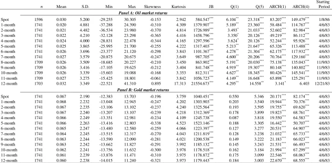
Key points of the data series under consideration are presented in Table 1, which

reports the mean, standard deviation, Kurtosis, Skewness, the Jarque-Bera normality test (JB),

the Ljung-Box first [Q(1)] and the fifth [Q(5)] autocorrelation tests, and the first [ARCH(1)]

and the fifth [ARCH(5)] order Lagrange multiplier (LM) tests for the autoregressive

conditional heteroskedasticity (ARCH) for oil and gold spot and futures contracts. The mean

of oil market returns is at its lowest for futures price but as for the spot prices there is a

gradual increase with the longest maturity of 12-month contracts with highest average price of

0.32. On the other hand, as for the mean of gold market returns, it is at its lowest with

5

maturity of 12-month contract for futures price but there is a gradual increase for spot prices,

with the lowest maturity of 1-months contract with the highest average price of 0.68. In terms

of volatility, oil market returns exhibit a more volatile structure than gold market returns.

Based on the negative values of the skewness, there is a higher possibility of large decreases

in returns, with one exception. The exception is that, considering oil market returns, the

12-month contract returns has a positive skewness estimate around 0.89. Based on the kurtosis

statistic, we observe fat-tailed distribution for all return series. As a more important finding,

the variables under consideration are skewed to left, with positive excess kurtosis, leading to

non-normal distributions, as shown by the strong rejection of Jarque-Bera statistic at 1%

significance level. The use of the causality-in-quantiles test is first justified by the fat-tailed

distributions of both returns. We observe significant serial correlation for oil market returns,

while significant serial correlation is not found for gold market returns, as suggested by

Ljung-Box statistic. There are ARCH (autoregressive conditional heteroscedasticity) effects

in all the return series, as shown by the autoregressive conditional

heteroskedasticity-Lagrange multiplier (ARCH-LM) statistic.

# Insert Table 1 in Here #

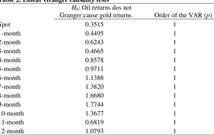
As well as examining the causality-in-quantiles from oil to gold, for completeness and

comparability, we also conducted the standard linear Granger causality test based on a linear

vector autoregression (VAR) model. Table 2 reports the results of linear Granger causality

tests. All of the F-statistics reported in Table 2 for the null hypothesis that oil returns does not

Granger cause gold returns are less than 1.8. Hence, we can conclude that even at significance

levels greater than 10%, there is no support of predictability running from oil to gold in a

linear VAR framework.

# Insert Table 2 in Here #

Subsequently, using the nonparametric quantile-in-causality approach, a

nonparametric (i.e., data-driven) approach, we examine the possibility of nonlinear

dependence between the oil returns and gold returns. In order to serve this purpose, Brock et

al. (1996, BDS) test is implemented on the residuals of an VAR(1) model for both returns.

We apply the BDS test to the residuals of oil returns and gold returns equation in the VAR(1)

dimensions (m), since there is strong evidence at the highest level of significance against

linearity. Based on this result, we conclude that there is strong evidence of nonlinearity in oil

returns and gold returns. This means that Granger causality tests in a linear framework might

lead to unreliable results due to misspecification errors. Because of the strong evidence of

nonlinearity, we implement the causality-in-quantiles test, which is deemed robust against,

jumps, outliers, structural breaks, and nonlinear dependence.

# Insert Table 3 in Here #

Given the strong evidence of nonlinearity obtained from the BDS tests, we further

investigate whether nonlinear Granger causality running from oil markets to gold markets

exists. In order to test for full sample nonlinear Granger causality, we use the nonlinear

Granger causality test of Diks and Panchenko (2006).6 Diks and Panchenko (2006) nonlinear Granger causality test results are presented in Table 4. We perform the tests for embedding

dimension m = 2, 3, 4 in order be robust against the lag order used in the test. The tests results

reported in Table 4 show that null hypothesis of no full sample nonlinear Granger causality

running from the oil to gold is rejected for none of the spot and futures markets. This results

holds unanimously for all embedding dimensions considered. Given the nonexistence of any

evidence on the full sample nonlinear Granger causality, we next turn to nonparametric

causality-in-quantiles tests, which considers all quantiles of the distribution not only the

center of the distribution.

# Insert Table 4 in Here #

The results of the quantile causality in mean and variance from the oil market series to

the gold market series are presented in Figure 2. The horizontal axis shows the quantiles and

the vertical axis shows the nonparametric causality test statistics corresponding to the quantile

in the horizontal axis. While 5% critical value is 1.96, 10 percent critical value is 1.64.

Horizontal thin solid lines show the critical value of 5% and thin two-dashed lines represent

10% critical values. There is clear difference between the quantile causality in mean and

quantile causality in variance analysis, as shown by the results in Figure 2. According to the

quantile causality test in mean the null hypothesis that oil does not Granger cause gold is not

6

rejected (p > 0.05) with a critical value of 1.96 over the quantile range of 0.25 to 0.60. The

only exception occurs at the quantile of 0.55. Except for one or two quantiles, the

causality-in-quantile test does reject the null hypothesis (p > 0.05) within the quantile range of 0.10 to

0.90 for future markets with differing maturities (1-month, 2-month, 3-month, 4-month,

6-month, 9-month). On the other hand, the null hypothesis that oil does not Granger cause gold

is rejected (p < 0.05) over the quantile range of 0.45 to 0.70 for futures market at 5-month

maturity as well as the quantile range of 0.25 to 0.65 for futures markets at 10-month and

11-month maturities, and the quantile range of 0.25 to 0.75 for futures market at 12-11-month

maturity. The quantile causality test in mean for the spot and futures markets at 5-month,

10-month, 11-10-month, and 12-month maturities exhibits that oil returns has predictive power on

gold returns. Yet, as for maturities of 1-month, 2-month, 3-month, 4-month, 6-month,

9-month, there is week evidence that oil returns have predictive power for gold returns for the

futures markets. For these maturities, oil has predictive power for gold only around the

quantiles from 0.40 to 0.60 and the null is rejected only at 10% level for the 3-month

maturity. In sum, oil returns have no predictive power for gold returns in bearish (lower

quantiles) and bullish (upper quantiles) market conditions.

According to the quantile causality in variance test results shown in Figure 2, the null

hypothesis that oil does not Granger cause gold in variance (2nd moment) is rejected (p < 0.05) over the quantile range of about from 0.15 to 0.75 for all spot and all futures markets.

This result shows that oil spot and all oil futures have strong predictive content for spot and

all future price volatility (variance) of gold market. Hence, there is no evidence supporting the

predictive power of oil for gold returns in the linear model. However, because of the

nonlinearity, the result of linear Granger causality is misleading. This in mind, nonparametric

causality-in-quantiles test results indicate that spot and future prices of oil have predictive

content for spot and future gold price volatility. This, in part, suggests that contrary to

equities, oil market moves in connection with gold market volatility during the periods of

stress.

The reason for this could be can be explained by the fact that crude oil is an essential

raw material in industrial manufacturing. Thus, global economic growth is much more linked

with crude oil than gold. For this reason, investors consider price changes in crude oil an

important phenomenon. With respect to global industrialization and globalization of markets,

world. The rapid development in alternative energy resources made it possible for the USA to

incorporate corn and white sugar in bioethanol in order to produce biodiesel fuel and this is an

example of the close link between crude oil prices and grease products, soybean and corns. In

summary, due to the extensive use of crude oil in the world global markets, the commodity

prices in world markets on the whole rest with the fluctuations of crude oil prices.

# Insert Figure 2 in Here #

The results in Figure 2 shows that the strength of the evidence of causality from oil

market to gold market, both in mean and variance, exhibits a hump-shaped pattern across

quantiles. Similar observations can be made across all the spot and 1- to 12-month maturities.

The hump-shaped pattern of causality is a new finding in this study and illustrates an

advantage of using our nonparametric causality-in-quantiles tests: A researcher who only

studies the median of the conditional distribution of gold returns and/or gold volatility would

likely to find strong evidence of predictive power from the oil to the gold, but, at the same

time, would completely miss that this evidence substantially weakens when the quantiles that

are farther away from the median are considered. We further point out that hump-shaped

curves in Figure 2 are asymmetric, where noncausality part is longer on the right tail and the

curves decline smoother on the right half of the figures. This implies that evidence of

noncausality is weaker on the right tail (extreme gold price increases) compared to the left tail

(extreme gold price decreases).

5. Conclusion

The extant literature so far has examined the oil market with respect to its predictive power

for gold markets. This paper adds to this literature by means of examining the predictability of

gold markets for the mean and volatility by the oil market. To serve this purpose, using

weekly data, standard linear Granger causality test is implemented but no evidence has been

found about causality running from oil market to gold market. Following the nonlinearity

tests, we find oil returns relationship with gold returns have nonlinear characteristics, which

suggests that the linear causality tests suffer from misspecification, thus yielding unreliable

results. In order to overcome this problem, we employ a nonparametric causality-in-quantiles

test, incorporating the test for nonlinear causality of k-th order developed by Nishiyama et al.

the causality-in-quantiles, enables us to examine causality-in-mean as well as the causality in

variance. In this way, even when there might be no causality in mean, we can still examine

the causality-in-variance (volatility). The nonparametric causality tests in mean indicate that

oil prices have a weak predictive content for gold market. Yet, the null hypothesis that oil

prices does not Granger cause gold price volatility for spot and the futures markets at all

maturities is strongly rejected for both spot and futures markets. The results on the nexus

between oil market and gold market, on the whole, underline the significance of detecting and

modeling nonlinearity when examining predictability via causal relationships.

The hump-shaped pattern in causality-in-quantiles tests we have found for causality

running from oil markets to gold markets, both for causality in mean and variance, highlights

the strong causal effects at the center of the conditional distribution of gold-price fluctuations.

In other words, the strongest effects of oil returns on gold returns and gold volatility may

occur on average, especially at higher data-frequencies (weekly data), in times of normal

rather than in times of exceptional movements of the gold price. However, this finding does

not rule out that singular events like the outbreak of a financial crisis or geopolitical

turbulences that trigger significant movements of the gold price, but it rather highlights that

investors and policymakers should study the entire conditional distribution of gold-price

movements when looking for causal effects of oil that operate, for example, in normal times

and in times of gold market turmoil. Similarly, an asymmetric hump-shaped pattern of

causality highlights that the strength of causality effects differs across the upper and lower

parts of the conditional distribution of gold-price movements.

As we pointed out, events such as important financial crisis or geopolitical events that

trigger significant gold price fluctuations are not ruled out by the strong causality evidence on

the center of the gold returns distribution, but it rather highlights that investors and

policymakers when looking for causal effects from oil to gold markets should consider the

entire conditional distribution of gold-price movements, not only the center of the distribution

which corresponds to low return periods. The asymmetric hump-shaped pattern of causality

running from oil to gold markets found in our study highlights that the strength of causality

effects differs across the upper and lower parts of the conditional distribution of gold price

movements. These results imply that investors should be aware that predictive power of oil

prices for the gold prices observed in normal times weakens during extreme market

managers, our results show that gold is a safe haven against extreme oil price movements, but

it not an effective hedge instrument against oil price during the normal market periods.

Investors should also know that oil precise would only indicate direction of gold price

movements during normal market periods, oil prices do fail to predict the extreme gold price

References

Abhyankar, A., Xu, B., Wang, J., 2013. Oil price shocks and the stock market: Evidence from Japan. Energy Journal 34, 199–222.

Abdelaziz, M., Chortareas, G., Cipollini, A., 2008. Stock prices, exchange rates, and oil: evidence from middle east oil-exporting countries. Soc. Sci. Res. Netw. 44, 1–27.

Arouri, M.E.H., Lahiani, A., Nguyen, D.K., 2015. World gold prices and stock returns in China: insights for hedging and diversification strategies. Econ. Model. 44, 273–282.

Asteriou, D., Bashmakova, Y., 2013. Assessing the impact of oil returns on emerging stock markets: a panel data approach for ten Central and Eastern European Countries. Energy Econ. 38, 204–211.

Awokuse, T.O., Yang, J., 2003. The information role of commodity prices in formulating monetary policy: a re-examination. Econ. Lett. 79, 219–224.

Balcilar, M., Gupta, R., Pierdzioch, C., 2016a. Does uncertainty move the gold price? New evidence from a nonparametric causality-in-quantiles test. Resources Policy 49, 74-80.

Balcilar, M., Bekiros, S., Gupta, R., 2016b. The role of news-based uncertainty indices in predicting oil markets: a hybrid nonparametric quantile causality method. Empirical Economics, forthcoming. DOI: 10.1007/s00181-016-1150-0.

Bampinas, G., Panagiotidis, T., 2015. On the relationship between oil and gold before and after financial crisis: linear, nonlinear and time-varying causality testing. Studies in Nonlinear Dynamics & Econometrics 19, 657-668.

Barisheff, N. (2005). The gold, oil and us dollar relationship.

http://www.kitco.com/ind/barisheff/apr222005.html, accessed on 2016-2-1.

Basher, S.A., Sadorsky, P., 2006. Oil price risk and emerging stock markets. Glob. Financ. J. 17, 224–251.

Beckmann, J., Czudaj, R., 2013. Oil and gold price dynamics in a multivariate coin- tegration framework. Int. Econ. Econ. Policy 10, 453–468.

Beckmann, J., Czudaj, R., Pilbeam, K., 2015. Causality and volatility patterns between gold prices and exchange rates. N. Am. J. Econ. Financ. 34, 292–300.

Bhunia, A., 2013. Cointegration and causal relationship among crude price, do- mestic gold price and financial variables: an evidence of BSE and NSE. J. Con- temp. Issues Bus. Res. 2 (1), 01–10.

Capie, F., Mills, T.C., Wood, G., 2005. Gold as a hedge against the dollar. J. Int. Financ. Mark. Inst. Money 15, 343–352.

Chang, H.F., Huang, L.C., Chin, M.C., 2013. Interactive relationships between crude oil prices, gold prices, and the NT–US dollar exchange rate—a Taiwan study. Energy Policy 63, 441–448.

Christiano, L.J., Eichenbaum, M., Evans, C., 1996. The effects of monetary policy shocks: evidence from the flow of funds. Rev. Econ. Stat. 78, 16–34.

Cologni, A., Manera, M., 2008. Oil prices, inflation and interest rates in a structural cointegrated VAR model for the G-7 countries. Energy Econ. 30, 856–888.

Cong, R.G., Wei, Y.M., Jiao, J.L., Fan, Y., 2008. Relationships between oil price shocks and stock market: an empirical analysis from China. Energy Policy 36, 3544–3553.

Cunado, J., Perez de Gracia, F., 2003. Do oil price shocks matter? Evidence for some european countries. Energy Econ. 25, 137–154.

Cunado, J., Perez de Gracia, F., 2005. Oil prices, economic activity and inflation: evidence for some asian countries. Q. Rev. Econ. Financ. 45, 65–83.

Cunado, J., de Gracia, F.P., 2014. Oil price shocks and stock market returns: evidence for some European countries. Energy Econ. 42, 365–377.

Degiannakis, S., Filis, G., Kizys, R., 2014. The effects of oil price shocks on stock market volatility: evidence from European data. Energy J. 35 (1), 35–56.

Diks C., Panchenko, V., 2006. A new statistic and practical guidelines for nonparametric Granger causality testing. Journal of Economic Dynamics & Control 30, 1647–1669.

Hammoudeh, S., Yuan, Y., 2008. Metal volatility in presence of oil and interest rate stocks. Energy Econ. 30, 606–620.

Hussin, M.Y.M., Muhammad, F., Razak, A.A., Tha, G.P., Marwan, N., 2013. The link between gold price, oil price and islamic stock market: experience from Ma- laysia. J. Stud. Soc. Sci. 4, 2.

Ghosh, S., 2011. Examining crude oil price-exchange rate nexus for India during the period of extreme oil price volatility. Appl. Energy 88, 1886–1889.

Ghosh, S., Kanjilal, K., 2016. Co-movement of international crude oil price and Indian stock market: Evidences from nonlinear cointegration tests. Energy Economics 53, 111–117.

Hooker, M.A., 2002. Are oil shocks inflationary? Asymmetric and nonlinear specifications versus changes in regime. Journal of Money Credit and Banking 34, 540–561.

Hiemstra, C., Jones, J., 1994. Testing for linear and nonlinear Granger causality in the stock price-volume relation. J. Finance 49, 1639–1664.

Hurvich, C. M., Tsai, C.-L., 1989. Regression and Time Series Model Selection in Small Samples. Biometrika 76, 297–307.

Jeong, K., Härdle, W.K., Song, S., 2012. A consistent nonparametric test for causality in quantile. Econom Theory 28, 861–887.

Kim, M.H., Dilts, D.A., 2011. The relationship of the value of the dollar, and the prices of gold and oil: a tale of asset risk. Econ. Bull. 31, 1151–1162.

Kilian, L., 2009. Not all oil price shocks are alike: Disentangling demand and supply shocks in the crude oil market. American Economic Review 99, 1053.

Kilian, L., Park, C., 2009. The impact of Oil Price shocks on the US stock market. Int. Econ. Rev. 50, 1267–1287.

Le, T., Chang, Y., 2011. Oil and Gold: Correlation or Causation? DEPOCEN Working Paper Series No. 22.2.

Lee, Y., Huang, Y., Yang, H., 2012. The asymmetric long-run relationship between crude oil and gold futures. Glob. J. Bus. Res. 6, 9–15.

Li, Q. and J.S. Racine (2004), “Cross-validated local linear nonparametric regression,” Statistica Sinica 14, 485-512.

Liao, S.J, Chen, J.T., 2008. The relationship among oil prices, gold prices and individual industrial sub indices in Thaiwan. Working Paper Presented at International Conference on Business and Information. Seoul, South Korea.

Melvin, M., Sultan, J., 1990. South African political unrest, oil prices, and the time varying risk premium in the fold futures market. Journal of Futures Markets 10, 103–111.

Mishra, A., 2004. Stock market and foreign exchange market in India: are they related? South Asia Econ. J. 5 (2), 209–232.

Mollick, A.V., Assefa, T.A., 2013. US stock returns and oil prices: the tale from daily data and the 2008–2009 financial crisis. Energy Econ. 36, 1–18.

Narayan, P.K., Narayan, S., Zheng, X., 2010. Gold and oil futures markets, are markets efficient? Applied Energy 87, 3299–3303.

Nishiyama, Y., Hitomi, K., Kawasaki, Y., and Jeong, K., (2011). A consistent nonparametric Test for nonlinear causality - specification in time series regression. Journal of Econometrics 165, 112-127.

Patel, S.A., 2013. Causal relationship between stock market indices and gold price: evidence from India. IUP J. Appl. Financ. 19, 99.

Pierdzioch, C., Risse, M., Rohloff, S., 2015. Fluctuations of the real exchange rate, real interest rates, and the dynamics of the price of gold in a small open economy. Empir. Econ., 1–19.

Racine, J.S., Li, Q., 2004. Nonparametric estimation of regression functions with both categorical and continuous data. Journal of Econometrics 119, 99-130.

Reboredo, J. C., 2013. Is gold a safe haven or a hedge for the US dollar? Implications for risk management. Journal of Banking & Finance 37, 2665-2676.

Reboredo, J.C., Rivera-Castro, M.A., 2014. Gold and exchange rates: downside risk and hedging at different investment horizons. Int. Rev. Econ. Financ. 34, 267–279.

Sari, R., Hammoudeh, S., Ewing, B.T., 2007. Dynamic relationships between oil and metal commodity futures prices. Geopolit. Energy 29, 2–13.

Sari, R., Hammoudeh, S., Soytas, U., 2010. Dynamics of oil price, precious metal prices, and exchange rate. Energy Economics 32, 351–362.

Simakova, J., 2011. Analysis of the relationships between oil and gold price. J. Financ. 51 (1), 651–662.

Sjaastad, L.A., 2008. The price of gold and the exchange rates: once again. Resour. Policy 33, 118–124.

Soytas, U., Sari, R., Hammoudeh, S., Hacihasanoglu, E., 2009. World oil prices, precious metal prices and macroeconomy in Turkey. Energy Policy 37, 5557–5566.

Tiwari, A.K., Sahadudheen, I., 2015. Understanding the nexus between oil and gold. Resour. Policy 46, 85-91.

Zhang, Yue-Jun, Wei, Yi-Ming, 2010. The crude oil market and the gold market: evidence for cointegration, causality and price discovery. Resour. Policy 35, 168–177.

22

Table 1. Descriptive statistics for returns (%)

n Mean S.D. Min Max Skewness Kurtosis JB Q(1) Q(5) ARCH(1) ARCH(4)

Starting Period

Panel A: Oil market returns

Spot 1596 0.030 5.200 -29.255 30.305 -0.153 2.942 584.547*** 6.104** 23.318*** 83.207*** 149.479*** 1/8/86 1-month 1741 0.020 4.881 -37.288 24.390 -0.310 4.309 1379.907*** _5.189** _23.360*** _58.484*** _114.767*** _4/6/83 2-month 1741 0.021 4.482 -36.534 23.980 -0.370 4.814 1726.989*** 3.493* 21.033*** 52.602*** 82.984*** 4/6/83 3-month 1741 0.022 4.210 -32.128 23.298 -0.365 4.416 1458.796*** _3.350* _20.126*** _49.219*** _86.112*** _4/6/83 4-month 1741 0.024 4.000 -28.831 22.478 -0.344 4.165 1297.596*** 3.624* 20.126*** 52.244*** 95.926*** 4/6/83 5-month 1741 0.025 3.865 -25.995 21.700 -0.255 4.222 1317.403*** 5.213** 21.647*** 65.326*** 113.488*** 4/6/83 6-month 1741 0.026 3.696 -23.377 21.120 -0.298 3.843 1101.367*** 4.278** 21.304*** 62.175*** 117.932*** 4/6/83 7-month 1741 0.027 3.579 -20.875 20.675 -0.247 3.649 987.705*** 4.600** 20.206*** 70.764*** 129.160*** 4/6/83 8-month 1709 0.026 3.509 -18.685 20.227 -0.210 3.450 863.902*** 5.191** 20.030*** 75.138*** 135.043*** 11/9/83 9-month 1709 0.026 3.416 -17.105 19.625 -0.212 3.404 841.748*** 4.919** 19.307*** 80.148*** 140.802*** 11/9/83 10-month 1709 0.026 3.339 -15.603 19.088 -0.168 3.353 812.311*** 4.627** 18.345*** 80.426*** 145.541*** 11/9/83 11-month 1709 0.027 3.275 -15.425 18.801 -0.061 3.842 1056.723*** _4.149** _16.648*** _65.898*** _125.291*** _11/9/83 12-month 1703 0.032 3.349 -22.521 41.310 0.895 17.313 21554.673*** 4.295** 14.558** 3.141* 6.403 12/21/83

Panel B: Gold market returns

Spot 1741 0.067 2.190 -12.383 13.703 -0.196 3.759 1040.451*** 0.550 5.346 20.171*** 82.174*** 4/6/83

1-month 1741 0.068 2.232 -13.048 12.945 -0.247 4.202 1303.903*** 0.203 3.540 19.944*** 70.376*** 4/6/83 2-month 1741 0.067 2.235 -13.106 13.102 -0.237 4.240 1325.564*** 0.193 3.595 19.755*** 69.620*** 4/6/83 3-month 1741 0.067 2.240 -13.207 13.107 -0.239 4.218 1312.369*** 0.178 3.899 19.823*** 68.761*** 4/6/83 4-month 1741 0.066 2.249 -13.351 12.981 -0.234 4.109 1245.738*** 0.087 3.818 19.550*** 64.583*** 4/6/83 5-month 1741 0.066 2.263 -13.416 12.803 -0.338 4.523 1523.146*** _{0.188 3.305 16.442}*** _50.707*** _4/6/83 6-month 1741 0.065 2.247 -13.480 12.580 -0.259 4.066 1223.397*** 0.127 3.277 20.531*** 64.907*** 4/6/83 7-month 1741 0.064 2.245 -13.515 12.317 -0.270 4.043 1211.819*** _{0.128 3.238 21.032}*** _65.733*** _4/6/83 8-month 1741 0.063 2.244 -13.590 12.090 -0.281 4.021 1200.538*** 0.149 3.222 21.183*** 66.023*** 4/6/83 9-month 1741 0.063 2.242 -13.662 11.827 -0.291 3.992 1185.132*** _{0.145 3.243 21.531}*** _66.493*** _4/6/83 10-month 1741 0.062 2.241 -13.756 11.632 -0.300 3.978 1178.518*** 0.162 3.184 21.994*** 67.299*** 4/6/83 11-month 1741 0.061 2.239 -13.876 11.471 -0.310 3.975 1178.872*** _{0.175 3.099 22.546}*** _68.063*** _4/6/83 12-month 1741 0.060 2.238 -14.015 11.240 -0.321 3.973 1179.443*** 0.184 3.003 22.670*** 68.555*** 4/6/83

Note: Table reports the descriptive statistics for the spot and futures (1- to 12-monh) returns (in percent) for the oil (Panel A) and gold (Panel B) markets. Sample period starts at the period given

Table 2. Linear Granger causality tests

H0: Oil returns dos not

Granger cause gold returns Order of the VAR (p)

Spot 0.3515 1

1-month 0.4495 1

2-month 0.6243 1

3-month 0.4665 1

4-month 0.8578 1

5-month 0.9711 1

6-month 1.1388 1

7-month 1.3820 1

8-month 1.6680 1

9-month 1.7744 1

10-month 1.3677 1

11-month 0.6819 1

12-month 1.0793 1

Note: The table reports the F-statistic for the no Granger causality restrictions imposed on a linear vector autoregressive (VAR) model under the null hypotheses H0. The order (p) of the VAR is

Table 3. [Brock et al. (1996)] BDS Test

m=2 m=3 m=4 m=5 m=6

Oil equation residuals

Spot 4.3366*** 6.3979*** 8.7684*** 12.0488*** 16.0429*** 1-month 2.8986*** 4.6127*** 6.4604*** 8.9956*** 12.0025*** 2-month 2.7707*** 4.5157*** 6.5014*** 9.0343*** 12.3810*** 3-month 2.8410*** 4.5077*** 6.5455*** 9.0949*** 12.4291*** 4-month 2.7309*** 4.4384*** 6.2019*** 8.4082*** 11.2339*** 5-month 3.0060*** 4.7500*** 6.5533*** 8.9485*** 12.0510*** 6-month 2.6507*** 4.4563*** 6.4262*** 9.0234*** 12.1425*** 7-month 2.6189*** 4.5234*** 6.6230*** 9.2676*** 12.3733*** 8-month 3.0602*** 5.1484*** 7.3224*** 10.2580*** 13.7494*** 9-month 3.1748*** 5.3310*** 7.5371*** 10.4716*** 14.1007*** 10-month 3.2983*** 5.4987*** 7.9570*** 11.0193*** 14.8379*** 11-month 3.3594*** 5.5370*** 7.9182*** 10.8389*** 14.5746*** 12-month 3.6148*** 5.5830*** 7.8992*** 10.8845*** 14.5896***

Gold returns equation residuals

Spot 4.3366*** 6.3979*** 8.7684*** 12.0488*** 16.0429*** 1-month 2.8986*** 4.6127*** 6.4604*** 8.9956*** 12.0025*** 2-month 2.7707*** 4.5157*** 6.5014*** 9.0343*** 12.3810*** 3-month 2.8410*** 4.5077*** 6.5455*** 9.0949*** 12.4291*** 4-month 2.7309*** 4.4384*** 6.2019*** 8.4082*** 11.2339*** 5-month 3.0060*** 4.7500*** 6.5533*** 8.9485*** 12.0510*** 6-month 2.6507*** 4.4563*** 6.4262*** 9.0234*** 12.1425*** 7-month 2.6189*** 4.5234*** 6.6230*** 9.2676*** 12.3733*** 8-month 3.0602*** 5.1484*** 7.3224*** 10.2580*** 13.7494*** 9-month 3.1748*** 5.3310*** 7.5371*** 10.4716*** 14.1007*** 10-month 3.2983*** 5.4987*** 7.9570*** 11.0193*** 14.8379*** 11-month 3.3594*** 5.5370*** 7.9182*** 10.8389*** 14.5746*** 12-month 3.6148*** 5.5830*** 7.8992*** 10.8845*** 14.5896***

Table 4. [Diks and Panchenko (2006)] Nonlinear Granger Causality Test

m=2 m=3 m=4

Test statistic p-value Test statistic p-value Test statistic p-value 1.255 0.105 0.640 0.261 0.041 0.484 0.762 0.223 -0.032 0.513 -1.231 0.891 0.579 0.281 0.249 0.402 -0.424 0.664 0.592 0.277 0.262 0.397 -0.583 0.720 0.537 0.296 -0.208 0.582 -0.156 0.562 -0.089 0.535 -0.246 0.597 0.008 0.497 0.436 0.331 0.060 0.476 0.273 0.393 0.552 0.291 0.028 0.489 0.564 0.286 0.730 0.233 -0.269 0.606 0.830 0.203 0.716 0.237 0.105 0.458 1.248 0.106 0.445 0.328 0.071 0.472 1.161 0.123 -0.132 0.553 -0.446 0.672 0.905 0.183 -0.828 0.796 -1.335 0.909 0.440 0.330

Figure 1. Time series plots of the spot and futures prices for the oil and gold markets

Figure 2. Causality in mean and variance from the oil market series to the gold market series