Munich Personal RePEc Archive
Oil supply and demand shocks and stock
price: Empirical evidence for some
OECD countries
Dhaoui, Abderrazak and Saidi, Youssef
University of Sousse, Tunisia, Bank Al-Maghrib, Rabat, Morocco
April 2015
Online at
https://mpra.ub.uni-muenchen.de/63616/
1
Oil supply and demand shocks and stock price: Empirical evidence for
some OECD countries
1Abderrazak DHAOUI
aUniversity of Reims Champagne Ardenne bUniversity of Sousse, Tunisia
Youssef SAIDI
c
Research Department, Bank Al-Maghrib, Rabat, Morocco
Abstract
This paper examines the interactive relationships between oil price shocks and stock market in 11 OECD countries using Vector Error Correction Models (VECM). Considering both world oil production and world oil prices to supervise for oil supply and oil demand shocks, strong evidence of sensitivity of stock market returns to the oil price shocks specifications is found. As for impulse response functions, it is found that the impact of oil price shocks substantially differs along the different countries and that the results also differ along the various oil shock specifications. Our finding suggests that oil supply shocks have a negative effect on stock market returns in the net oil importing OECD countries. However, the stock market returns are negatively impacted by oil demand shocks in the oil importing OECD countries, and positively impacted in the oil exporting OECD countries.
Keywords: Oil price; Stock market return; Oil supply shocks; Oil demand shocks, Vector Error Correction Models.
JEL Classification: G12; Q43.
1
The views expressed herein are those of the authors and do not necessarily reflect the views of their institutions. a
UFR Sciences Economiques et de Gestion; Address: 57 rue Pierre Taittinger 51096 Reims cedex. b
Corresponding author; Department of Econometrics and Management, Faculty of Economic Sciences and Management; Address: Erriadh city - 4023 (Sousse) Tunisia. E-mail: abderrazak.dhaoui@fsegs.rnu.tn c
2
Introduction
Oil price has experienced a series of shocks for more than fifty years. These shocks are not without impact on the industrial sector and therefore on economic growth and financial stock market development. More specifically high fluctuations in oil prices may asymmetrically influence stock market returns. The sensitivity of stock prices to oil price shocks have been the subject of many works such as those of Jones and Kaul (1996), Sadorsky (1999), Huang et al. (1996), El-Sharif et al. (2005), Naifar and Al Dohaiman (2013),Chang and Yu (2013),Mohanty, et al. (2011), and Nguyen and Bhatti (2012).
Huang et al. (1996) results indicate non-significant sensitivity of stock returns to oil price shocks for some specific markets such as that of the S&P 500 stock market. However, several studies such as those of Nandha and Faff (2008), Papapetrou (2001), Sadorsky (1999), Issac and Ratti (2009), and Shimon and Raphael (2006) show negative connections between stock returns and oil price increases.
To supervise the stock returns behavior following the changes in oil price, different studies added other variables allowing the investigation of the direct and indirect connections between oil price shocks and stock returns. Among others oil production is introduced as an explanatory variable by Kilian (2009), Kilian and Park (2009) and Güntner (2013). Bernanke et al. (1997) and Lee et al. (2012) introduced the short-term interest rate. Sadorsky (1999), Park and Ratti (2008) and Cunado and Perez de Gracia (2003, 2005, 2014) developed models that associate the stock returns to the different variables including oil price, short-term interest rate and industrial production.
The aim of this study is to examine the response of stock returns to oil shocks expressed in both world and local real prices. The contribution of this paper is twofold. First, by using a long data span we allow for possibility of a structure break. Second, in this paper we consider different oil price specifications together with variables measuring industrial production indexes and short term interest rates which help supervising for the different channels through which oil price could influence the evolution of stock prices. Especially, one limitation of the existing empirical studies is to take into account only the global effect of oil price shocks. One of the important contributions of this paper is to consider both demand shock and supply shocks in order to supervise for the sensitivity of stock returns to each of them.
3
The remainders of this paper proceed as follows. Section 2, reviews the literature on the sensitivity of stock market returns to oil price shocks. Section 3 focuses on the empirical analysis. In this section we present the variable definitions and the modeling approach. The discussion of empirical findings is the subject of the section 4. Finally, section 5 provides summary and discusses concluding observations and implications.
2.
Literature review
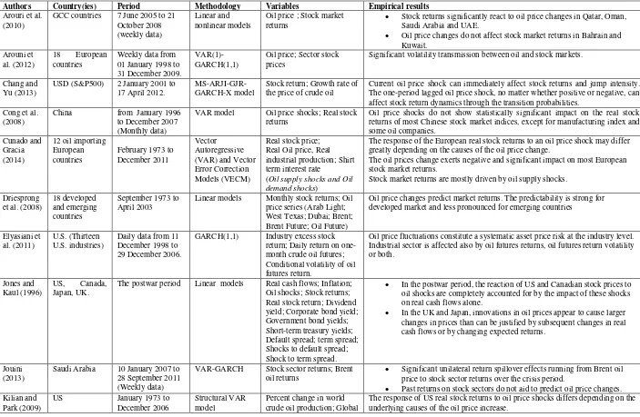
Several studies have focused on the nature of relationship between oil price changes and stock market returns. The results of these studies are mixed and no consensus is identified. This can be attributed to the fact of using different data, period and methodological approaches. Table 1 displayed the chronological list of the empirical studies on the connection between oil price and stock returns. In this Table, columns 1 to 6 present the author(s), country, period, methodology, variables, and empirical results, respectively. These studies show that the results are conflicting and mixed across different countries.
[Insert Table 1 about here]
The linkages between oil price and stock returns has come to the forefront of public attention and this potentially because of the increase in uncertainty of the energy sector, that impacts directly and indirectly the financial markets. The problems have caused there to be a concern with a re-examination of what exactly can be the explication of the negative connection between oil price shocks and the stock returns. The negative reaction of real stock prices to the increase in oil prices is attributed according to several authors to the direct effects of this increase in terms of cash flows and inflation. This argument is shared by several authors who document that oil price shocks lead to rising inflation and unemployment and therefore depress macroeconomic growth and financial assets (Shimon and Raphael, 2006). In fact, the oil price can corporate cash flow since oil price constitutes a substantial input in production. In addition, oil price changes can influence significantly the supply and demand for output at industry sector and even at the whole economy level and therefore decrease the firm performance through its effect on the discount rate for cash flow because the direct effect that may exert on the expected rate of inflation and the expected real interest rate. These direct and indirect effects of the high volatility in oil prices seem likely to increase uncertainty at firms and in the economy. In this line, Bernanke (1983) and Pindyck (1991) argue that higher change in energy prices creates uncertainty about future energy price and incites, consequently, firms to postpone irreversible investment decisions in reaction to the profit prospects. The negative reaction of real stock prices to the increase in oil prices is also confirmed in O‟Neil et al. (2008) for US, UK and France, Park and Ratti (2008) for US and 12 European oil importing countries, and Nandha and Faff (2008) for global industry indices (except for attractive industries). Ciner (2001) introduced nonlinear effects and confirms the same results according to which there is a significant negative connection between oil price shocks and real stock returns.
4
Using quarterly data for Canada, Japan, the UK and the US over the period spanning 1947 to 1991, Jones and Kaul (1996) found a serious reaction of stock prices to oil price shocks in the US and Canada. They explained this reaction in terms of the effects that induce these shocks to real cash flows. Results for the Japan and the UK are without important significance.
Other studies show in contrast non-significant connections between oil price shocks and stock market returns. Chen et al. (1986) found that the returns generated by oil futures are without significant impact on stock market indices such as S&P 500, and there is no gain in considering the risk caused by the excessive volatility of oil prices on stock markets. In the same line Apergis and Miller (2009) obtained results that do not support a large effect of structural oil market shocks on stock returns in eight developed countries.
Several other authors explored the relationship between stock market and oil price changes using Vector Autoregressive (VAR) model. Despite Huang et al. (1996) found that daily oil futures returns present no significant effect on the broad-based market indexes such as the S&P 500 over the period 1979-1990, Sadorsky (1999) results obtained using an unrestricted VAR model including monthly data of oil prices, stock returns, short-term interest rate, and industrial production spanning the period from 1947 to 1996 show that oil price played a pivotal role in explaining the US broad-based stock returns. This result is confirmed in Park and Ratti (2008) using monthly data for the US and 13 European countries over the period from January 1986 to December 2005. Their findings confirm that oil price shocks exert a statistically significant impact on real stock returns in the same month or within one month.
More recently, Naifar and Al Dohaiman (2013) have investigated, in a first time, the impact of both change and volatility of oil price variables on stock market returns under regime shifts in the case of Gulf Cooperation Council (GCC) countries. They employed a Markov regime-switching model to generate regime probabilities for oil market variables. Two-state Markov switching models have been used what are the crisis regime and non-crisis regime. In a second time, they investigated the non-linear interdependence between oil price, interest rates and inflation rates before and during the subprime crisis. They considered various Archimendean copula models with different tail dependence structures. Their results show evidence supporting a regime dependent relationship between GCC stock market returns and OPEC oil market volatility with exception to the case of Oman. The findings show also an asymmetric dependence structure between inflation rates and crude oil price and that this structure orients toward the upper side during the recent financial crisis. The authors found moreover a significant symmetric dependence between crude oil prices and the short-term interest rate during the financial crisis.
In the same vein, Aloui and Jammazi (2009) developed a two regime Markov-switching EGARCH model to examine the interdependence between crude oil shocks and stock returns. They used monthly data for France, UK and Japan over the period from January 1987 to December 2007. The main result of their study supports that net oil prices play a pivotal role in determining firstly the volatility of real returns and secondly the probability of transition across regimes.
5
Taken together these findings confirm those of Papapetrou (2001) using 1989-1999 monthly data of the Greek stock market who reports, in fact, that oil price forms an important component in explaining stock price movements, and the increases in oil price shocks induce serious depressions in real stock returns.
Similarly, Issac and Ratti (2009) used a Vector Error Correction model for six OECD countries over the period spanning January 1971 to March 2008 to test the long-run relationship between the world price of crude oil and international stock markets. Their results confirm a clear long-run connection between oil price and real stock market returns supporting the negative reaction of real stock prices to the increase in oil prices.
Reboredo and Rivera-Castro (2013) used daily data for the aggregate S&P 500 and Dow Jones Stoxx Europe 600 indexes and US and European industrial sectors (automobile and parts, banks, chemical, oil and gas, industrial goods, utilities, telecommunications, and technologies) over the period from 01 June 2000 to 29 July 2011 to examine the connection between oil prices and stock market returns. The results of the wavelet multi-resolution analysis show that oil price changes have no much effect on stock market returns in the pre-crisis period at either the aggregate as well as the sectoral level. With the onset of the financial crisis, the results support the positive interdependence between oil price shocks and the stock returns at both the aggregate and the sectoral level.
3.
Data and Methodology
3.1 Data description
To examine the empirical linkages between oil price shocks and stock market returns in 11 OECD countries, we collect data for real stock prices, real industrial production, nominal interest rates and oil prices over the period from January 1990 to December 2013. The countries included in our analysis are Canada, Czech Republic, Denmark, Hungary, Korea, Mexico, Norway, Poland, Sweden, UK and US. Following empirical studies, all data used in this article are monthly. Thus, the starting date of the sample period is determined by the availability of monthly data serving to compute our variables for each country. The following notations will be used in the rest of the paper:
rsp real stock prices,
rip real industrial production,
r short-term interest rate,
op real oil price (world or national),
yoil real oil production (world or national).
Other papers that also use monthly data are those of Sadorsky (1999), Park and Ratti (2008), Driesprong et al. (2008), Lee et al. (2012), and Cunado and Perez de Gracia (2014) among others. The variables used in our model are computed as follows.
Real stock prices. The real stock price is computed as the stock prices deflated by the consumer
price index. The data for stock market indices are compiled by “OECD” and “EUROSTAT”
6
( ( ) ( )) , where Pt represents the real stock market index at the time t. To
avoid the impact of the inflation rate we use approximately the real stock returns instead of the returns calculated for each market. This proxy for the real stock return is already used by Park and Ratti (2008) and Cunado and Perez De Gracia (2014).
Real national (resp. world) oil prices. In this paper we use the real national price for each country as a proxy for the oil price. The real national price is computed as the product of the nominal oil price and the exchange rate deflated by the consumer price index of each country. The UK Brent nominal price is used as proxy for the nominal oil price. This proxy is commonly used by several authors such as Cunado and Perez de Gracia, (2003, 2005, 2014) and Engemann et al., (2011) in order to investigate the type of interconnections between oil shocks and macroeconomic variables. In addition, we define the world real oil price as the nominal oil price deflated by the US producer price index.
Real industrial production. Based on the works of Sadorsky (1999), Park and Ratti (2008) and Cunado and Perez de Gracia (2014), the real industrial production is computed as the nominal industrial production deflated by the consumer price index of each country.
Oil price, oil production, industrial production and short term interest rates are included in the analysis to supervise the stock market behavior after the oil price shocks. Further, the use of oil production variable together with the oil price is motivated by the wish to benefit from the dispersion between oil supply and oil demand shocks. This variable is earlier used by Kilian (2009), Kilian and Park (2009) and Güntner (2013).
The data for the oil price and the oil production are obtained from the Energy Information Administration (EIA) database and the International Financial Statistics (International Monetary Fund). Finally the data for the macroeconomic variables (Industrial production, producer price index, consumer price index, Short-term interest rates and exchange rate) are compiled by the
“OECD” database and the Global Financial Data (GFD).
Indirect effects of oil price shocks on real stock returns are supervised based on two variables commonly used in previous studies. For Bernanke et al. (1997), Sadorsky (1999), Park and Ratti (2008) and Lee et al. (2012) and Cunado and Perez de Gracia, (2014), the short-term interest rate constitutes a good proxy that allows monitoring the connections between oil price shocks on stock returns. The use of this variable is motivated by the fact that central bank react sensitively to higher oil prices through the short-term nominal interest rate. This reaction induces an indirect effect of oil price shocks on real economic activity and therefore on real stock market returns. The second indirect effect of the oil price shocks on the real economic activity and therefore the real stock returns can be supervised using the industrial production variable.
Oil supply (resp., demand) shocks. Recent studies by Killian (2009), and Peersman and Van Robays (2009) distinguish between three different types of oil shocks. They consider that the effect of oil price changes can be supervised using separately oil supply shocks, oil demand shocks driven by the global economic activity and oil specific demand shocks.
Following the idea that “not all oil price shock are alike” (Killian, 2009), in this paper the analyses
will be based on the specification proposed by Cunado and Perez de Gracia (2014). This specification can be presented as follows.
Let Δopt = opt – opt-1. This relation specifies the Oil price variations defined as the first log
7
production changes defined as the first log difference of world real oil production. The oil supply shocks (Osst) and oil demand shocks (Odst) will be computed respectively as follows.
{ ( ) ( ) (1)
{ ( ) ( ) (2)
In other words, an oil price increase (decrease) together with world oil production increase (decrease) will be identified as demand shock. In other case, an oil price increase (decrease) followed by a world oil production decrease (increase) will be identified as a supply shocks. We consider here that the different type of oil price shocks can have separate effects on the economy and hence on the stock returns.
3.2 Methodology
The primary interest of this study is to investigate the effects of oil shocks- expressed in both world and national real prices- on stock returns in 11 OECD countries using the Vector Error Correction (VECM) model introduced by Johansen (1988) and alternatively Vector autoregressive (VAR) methodology proposed by Sims (1980). The advantage of the cointegration procedure of Johansen and Joselius (1990) is that it allows firstly testing for the existence of one or more cointegration relationships between the different series. Second, the Johansen method is a multivariable test that allows determining the number of cointegration relationships between the selected series. The VECM contains the cointegration relation built into the specification so that it restricts the long-run behavior of the endogenous variable to converge to its cointegrating relationship while allowing for short-run adjustment dynamics.
Thus, this approach avoids the two-stage tests applied in the Engel-Granger procedure that allows having a single cointegration relationship. This approach also has the advantage to take into account the problem of simultaneity. Finally, the assumption of exogeneity of the variables is not supported and there is no need to impose restrictions on the estimated coefficients to determine the short-term relationships.
Consider a VECM model based on monthly data for yt= (rspt, ript, rt, opt) given by:
∑ (3)
Where ∆ is the difference operator, B0 is a 4-dimensional column vector of deterministic constant
terms and (Bi) i=1, …, p denotes 4-order matrices of short-run information parameters. αβ’ is a
8
cointegrated, in this case, and the variables have first to be differenced and one has a VAR in difference.
In the first step, we use the conventional unit root tests of Dickey-Fuller (ADF), Phillips-Perron (PP) and KPSS tests to verify the stationarity of all variables. In a second time, we apply the
endogenous breaks LM unit root test of Lee and Strazicich (2003, 2004) to avoid „spurious rejections‟ from the conventional unit root tests.
Since each of the variables real stock prices, real industrial production, nominal interest rates and real national (resp., world) oil prices contains a unit root, we proceed in the second step to determine the lag length of the VAR version of the VEC model using the Akaike Information Criterion (AIC). Then, we apply the Johansen‟s cointegration test to determine the number of cointegrating vectors (rank (αβ’) = r) using two different likelihood ratio statistics (LR): the trace statistic and the maximum eigenvalue statistic. In the third step, the VEC model is estimated by the maximum likelihood method. Finally, we analyze the impact of oil price changes on stock markets by examining the impulse response functions (IRFs) obtained by estimating the previous VECM.
4.
Empirical results
4.1 Data preliminary analysis
4.1.1 Unit root
For the 11 OECD countries, the outcome of ADF, Phillips-Perron and KPSS unit root tests in level and in the first difference of the real stock prices, short-term interest rate, real industrial production and real oil (national and world) prices are presented in Table 2.
[Insert Table 2 about here]
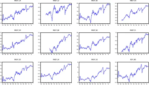
Results in Table 2 show that about all variables are integrated of order one with the exception for the real oil price which seems, in a first look, to be trend stationary in level for Canada, Korea, Mexico, Poland and Sweden. However this result can be carefully taken into account. In fact, the plot of real national oil price time series shows for each country that the series are not really trend stationary in level. The history, shown in Figure 1, of the real national oil prices indicates the presence of breaks in all oil price series.
[Insert Figure 1 about here]
9
search for a break point and test for the presence of a unit root when the process has a broken constant or trend and have demonstrated that their tests are robust and more powerful than the conventional unit root tests. To avoid this problem and to examine the potential presence of breaks, we use in this paper the endogenous two-break LM unit root tests proposed by Lee and Strazicich (2003, 2004). This later seems to be unaffected by breaks under the null hypothesis. Table 3 shows the results of applying endogenous break LM unit root test. We find as anticipated significant structural breaks of real national oil prices of Canada, Korea, Poland and Sweden but not for Mexico. For this last country, the time series of real national oil price seems to be linear trend stationary potentially because of the shortness of data. Regarding the ADF, PP, KPSS and LM unit root tests, the results conclude in favor of unit root for all level series used in all countries VECM data.
[Insert Table 3 about here]
4.1.2 Cointegration
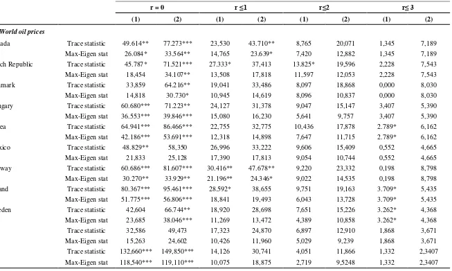
Assuming that all variables contain a unit root, we test then for cointegration in each VECM using both the trace and the maximum eigenvalue tests. Results of applying the Johansen and Juselius (1990) approach are shown in Table 4. The Table includes the ranks given in the first line, the number of cointegration vectors in line 2 and eigenvalues and trace statistics for each selected country. The critical value is mentioned using asterisks. The null hypothesis is that the number of
cointegrating relationship is equal to r, which is given in the “maximum rank” observed in the first
line of the Table 4. The alternative is that there are more than r cointegrating relationships. We reject the null if the trace statistic is greater than the critical value. We start by testing H0: r=0. If this null hypothesis is rejected, we repeat for H0: r=1. The process continue for r=2, r =3, etc. The process stops when a test is not rejected. The existing of one or more cointegration vectors explains that the variables have a long run relationship and we should continue to use VECM (Vector Error Correction Model).
[Insert Table 4 about here]
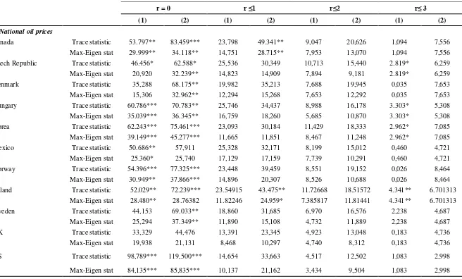
Results displayed in the first part (World oil prices) of Table 4 show that there is at least one cointegration vector with an intercept and/or trend in all countries except for UK for which we find one cointegration vector without constant. Consequently we can conclude that there is at least one cointegration vector for all selected countries. In the second part (national oil prices) of Table 4 the null hypothesis of no cointegration is not rejected only for UK (at 5% level of significance). Looking at the Johansen cointegration test results, we conclude that the VECM can be applied to all countries except for the UK (r=0) under the “all shock” specification of world oil prices. For this last case, we use consequently a VAR model (r=0).
4.2 Impact of oil price shock on stock market
10
2005, 2014) among others, each processes contains the variables stock prices, real industrial production indexes, short-term interest rates and different specifications for oil price shocks: (i) national real oil price; (ii) national oil price as defined in (1) and (2) ; (iii) world real oil price; (iv) world oil price as defined in (1) and (2).
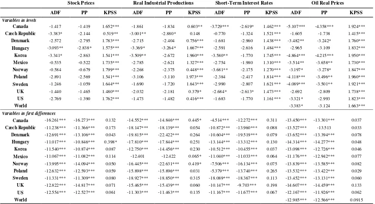
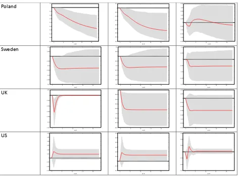
Using the above estimated models, we use impulse response functions to analyze the impact of three types of real oil price shocks on real stock returns: all oil price shocks, oil demand price shocks and oil supply price shocks. To compute the impulse response functions (IRFs) the disturbances from the moving average (reduced form) representation of each VECM model are then orthogonalised using the Cholesky decomposition.
In this section we analyze the impact of world real oil price shock on real stock returns by examining impulse response functions. Figures 2 and 3 show the impulse response of real stock returns resulting respectively from one standard deviation (1SD) shock to oil prices measured by the log of world and national real oil prices from VECM (rspt, ript, rt, opt) estimated for 11 OECD countries. The three columns of each figure describe respectively the effect of positive real oil all shock, real oil demand shock, and real oil supply shock. Monte Carlo constructed 95% confidence bounds are provided to judge the statistical significance of the impulse response functions. Like previous empirical works focusing on separate oil price shocks into different demand and supply components (see, for example, Kilian and Park, 2009; Apergis and Miller, 2009; Güntner, 2013; Cunado and Perez de Gracia, 2014), we also find that the impact of real oil changes on the 11 OECD countries real stock returns may differ depending on the nature of the oil shock. The main results are presented for world and national oil price shocks as follows.
4.2.1 World real oil price shock
Figure 2 shows that world oil price shocks (first column) have a negative significant effect on stock market returns in UK, Czech Republic, Denmark, Korea, Mexico, Poland and Sweden, while they have a positive effect only in USA and Hungary. The effect on stock returns in Canada is, however, not significant. For the stock market returns in Norway the impact is mixed, that is negative in third and fourth month and positive in the second year.
11
On concluding the discussion of this subsection, it should be noted that the net oil importing countries (UK, USA, Czech Republic, Korea, and Sweden) are impacted negatively by oil supply shocks except for Hungry, while the net oil exporting countries (Denmark, Norway, Mexico) are not impacted by oil supply shocks except for Canada (positive effect). On the other hand, both net oil exporting and importing countries (UK, Czech Republic, Denmark, Korea, Mexico, Norway, Poland and Sweden) are negatively impacted by oil demand shocks except for USA, Canada and Hungry (positive effect).
[Insert Figure 2 about here]
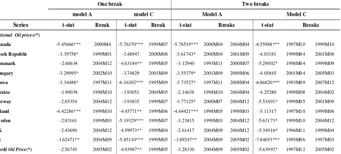
4.2.2 National real oil price shock
In this sub-section, we examine the impact of national real oil price shocks on real stock returns. Figure 3 shows that national oil price shocks have significant negative effects on stock returns in UK, Canada, Czech Republic, Denmark, Korea, Mexico, Norway, Poland and Sweden, while they have a positive effect on stock returns in USA and Hungry.
Next, when decomposing oil price in demand and supply shocks, we also find that national oil demand and oil supply shocks have different impact on real stock returns. Comparing columns two and three in Figure 3, we find that oil demand shocks have negative effects in UK, USA, Czech Republic, Korea, Poland and Sweden, while they have a positive effect on stock returns only in Denmark, Hungry and Norway. The effects on stock returns in Canada and Mexico are, however, not significant.
Nonetheless, oil supply shocks have significant negative impact on stock returns in UK, USA, Canada, Czech Republic, Denmark and Mexico, while they have a positive effect on stock returns in Hungry, Korea, and Sweden. The effects on stock returns in Norway and Poland are, however, not significant. A similar result for UK stock market can be found in Apergis and Miller (2009), Kilian and Park (2009), Güntner (2013), and Cunado and Perez de Gracia (2014).
The chief results, in this sub-section, can be summarized as follows. First, oil demand shocks have a negative effect in the net oil importing countries (UK, USA, Czech Republic, Korea, Poland and Sweden) except for Hungry, while the net oil exporting countries (Denmark, Norway) are positively impacted by oil demand shocks except for Canada and Mexico (no effect). Second, oil supply shocks have a negative effect in both net oil exporting and importing countries (UK, USA, Canada, Czech Republic, Denmark and Mexico) except for Hungry, Korea, and Sweden (positive effect). Thus, we note here that the oil supply shocks have not effect in Norway and Poland.
[Insert Figure 3 about here]
5.
Policy implication and conclusion
12
operating costs and therefore an increase in prices. The reaction of real stock prices to the increase (decrease) in oil price is attributed accordingly to the direct effects of this increase (decrease) in terms of cash flows and inflation. Oil price shocks lead to raising inflation and therefore depress macroeconomic growth and financial assets. In fact, oil price can corporate cash flow since oil price constitutes a substantial input in production. In addition, oil price changes can influence significantly the supply and demand for output and therefore decrease the firm performance through its effect on the discount rate for cash flow because the direct effect that may exert on the expected rate of inflation and the expected real interest rate.
The paper examines the extent to which supply and demand oil price shocks have different effects on stock returns in 11 OECD countries (UK, USA, Canada, Czech Republic, Denmark, Hungary, Korea, Mexico, Norway, Poland and Sweden) over the period from January 1990 to December 2013. We utilize a cointegration vector error correction model with additional macroeconomic variables to investigate the direct and indirect connections between oil price shocks and stock returns.
First, we find clear long-run relationship between real stock prices and real oil prices measured by world and local prices in all countries except for the case of world prices in UK. Thus, the short-term dynamics between oil prices and stock prices are analyzed using impulse response functions. The results in this paper show that the effect of real oil changes on real stock returns in the considered 11 OECD countries may differ depending on the nature of the oil shock. Our findings results show that the impact of oil price shocks substantially differs along the countries and that the significance of the results also differs along the oil prices specification (real national oil price, real world oil price, supply shocks, demand shocks).
As predicted in previous studies, the empirical evidence support that oil price shocks contributes significantly to systematic risk at the financial market level. The response of stock returns to oil price shocks can be attributed to their impact on current and expected futures real cash flows. Our finding suggest, thus, that oil supply shocks have a negative effect on stock market returns in the net oil importing OECD countries since oil represents an essential input and the increase in oil prices induce a raise in industrial costs. However, the stock markets are negatively impacted by oil demand shocks in the oil importing OECD countries due to a higher energy costs, and positively impacted in the oil exporting OECD countries due to the perspective of increasing world income and consumption. Finally, oil demand shocks have only negative effect on stock markets in most of the net oil exporting and importing OECD countries.
References
Aloui, C. and Jammazi, R. (2009), “The effects of crude oil shocks on stock market shifts behavior:
A regime switching approach”,Energy Economics, vol. 31, pp. 789-799.
Apergis, N. and Miller, S.M., (2009), “Do structural oil-market shocks affect stock prices?”, Energy
13
Arouri, M., Dinh, T.H., & Nguyen, D.K. (2010), “Time-varying predictability in crude oil markets: The case of GCC countries”, Energy Policy, 38, 4371–4380.
Arouri, M.E.H., Jouini, J., Nguyen, D.K., (2012), “On the impacts of oil price fluctuations on European equity markets: volatility spillover and hedging effectiveness”, Energy Economics. 34, 611–617.
Basher, S.A. and Sadorsky, P., (2006), “Oil price risk and emerging stock markets”, Global Finance Journal, vol. 17, pp. 224-251.
Bernanke, B.S., (1983), “Irreversibility, uncertainty, and cyclical investment”, Quarterly Journal of
Economics, vol. 98, pp. 115-134.
Bernanke, B.S., Gertler, M., and Watson, M.W., (1997), “Systematic monetary policy and the
effects of oil shocks”,Brookings Papers on Economic. Activity, vol. 1, pp. 91-157.
Chang, K.L., and Yu, S.T., (2013), “Does crude oil price play an important role in explaining stock
return behavior?”,Energy Economics, vol. 39, pp. 159-168.
Chen, N., Roll, R., Ross, S.A., (1986), “Economic forces and the stock market”, The Journal of
Business, vol. 59, Issue 3, pp. 383-403.
Christiano, L.J., (1992), “Searching for breaks in GNP”, Journal of Business and Economic Statistics, vol. 10, pp. 237–250.
Ciner, C., (2001), “Energy shocks and financial markets: nonlinear linkages”, Studies in Non-linear
Dynamics and Econometrics, vol. 5, pp. 203-212.
Cong, R.G., Wei, Y.M., Jiao, J.L., Fan, Y., (2008), “Relationships between oil price shocks and stock market: an empirical analysis from China”,Energy Policy, vol. 36, 3544–3553.
Cunado, J., and Perez de Gracia, F., (2003), “Do oil price shocks matter? Evidence for some
European countries”, Energy Econmics, vol 25, pp. 137-154.
Cunado, J., and Perez de Gracia, F., (2005), “Oil prices, economic activity and inflation: evidence
for some Asian economies”. The Quarterly Review of Economics and Finance, vol. 45, pp. 65-83.
Cunado, J., and Perez de Gracia, F., (2014), “Oil price shocks and stock market returns: Evidence
for some European countries”, Energy Econmics, vol. 42, pp. 365-377.
Driesprong, G., Jacobsen, B., and Maat B., (2008), “Striking Oil: Another Puzzle?”, Journal of Financial Economics, vol. 89, n° 2, pp. 307-327
El-Sharif, I., Brown, D., Burton, B., Nixon, B., and Russell, A., (2005), “Evidence on the nature and
extent of the relationship between oil prices and equity values in the UK”. Energy Economics, vol.
27, pp. 819-830.
Elyasiani, E., Mansur, I., Odusami, B., (2011), “Oil price shocks and industry stock returns”,
14
Engemann, K.M., Kliesen, K.L., and Owyang, M.T., (2011), “Do oil shocks drive business cycle?
Some US and international evidence”,Macroeconomic Dynamics, vol. 15, pp. 298-517.
Güntner, J.H., (2013), “How do international stock markets responds to oil demand and supply
shocks?”,Macroeconomic Dynamics, First View Article, pp. 1-26.
DOI:http://dx.doi.org/10.1017/S1365100513000084.
Hong, H., Torous, W., and Valkanov, R., (2002), “Do Industries Lead the Stock Market? Gradual
Diffusion of Information and Cross-Asset Return Predictability”, Working Paper, Stanford University& UCLA
Huang, R., Masulis, R.W., Stoll, H.R., (1996), “Energy Shocks and Financial Markets”, Journal of
Futures Markets, vol. 16, Issue 1, pp. 1-27.
Issac, M.J., and Ratti, R.A., (2009), “Crude Oil and stock markets: Stability, instability, and
bubbles”, Energy Economics, vol. 31, pp. 559-568.
Johansen, S., (1988), “Statistical analysis of cointegrating vectors”. Journal of Economic Dynamics Control, vol.12, 231–254.
Johansen, S., Juselius, K., (1990), “Maximum likelihood estimation and inference on cointegration with applications to demand for money”, Oxford Bulletin Economics and Statistics, vol. 52, pp. 169–210.
Jones, C.M., and Kaul, G., (1996), “Oil and the Stock Market”, Journal of Finance, vol. 51, n° 2,pp. 463-491.
Jouini, J., (2013), “Return and volatility interaction between oil prices and stock markets in Saudi
Arabia”, Journal of Policy Modeling, vol. 35, pp. 1124-1144.
Kilian, L., (2009), “Not all oil price shocks are alike: disentangling demand and supply shocks in
the crude oil market”, American Economic Review, vol. 99, n° 3, pp. 1053-1069.
Kilian, L., Park, C., (2009), “The impact of oil price shocks on the US stock market”, International
Economic Review, vol. 50, Issue 4, pp. 1267-1287.
Lee, B.J., Yang, C.H., and Huang, B.H., (2012), “Oil price movements and stock market revisited: a
case of sector stock price indexes in the G7 countries”, Energy Economics, vol. 34, pp. 1284-1300.
Lee, J., Strazicich, M.C., (2001), “Break point estimation and spurious rejections with endogenous unit root tests”. Oxford Bulletin Economics and Statistics, vol. 63, pp. 535–558.
Lee, J., Strazicich, M.C., (2003), “Minimum LM Unit Root Test with Two Structural Breaks.” Review of Economics and Statistics, vol. 85, n° 4, pp. 1082-1089.
Lee, J., Strazicich, M.C., (2004) “Minimum LM unit root test with one structural break” Working
Paper 04-17, Department of Economics, Appalachian State University, Boone, North Carolina.
Lee, Y.H., and Chiou, J.S., (2011), “Oil sensitivity and its asymmetric impact on the stock market”,
15
Mohanty, S.K., Nandha, M., Turkistani, A.Q., and Alaitani, M.Y., (2011), “Oil price movements and stock market returns: Evidence from Gulf Cooperation Council (GCC) countries” Global Finance Journal, vol. 22, pp. 42-55.
Naifar, N., and Al Dohaiman, M.S.,(2013), “Nonlinear analysis among crude oil prices, stock
markets‟ return and macroeconomic variables”, International Review of Economics and Finance,
vol. 27, pp. 416-431.
Nandha, M., and Faff, R., (2008), “Does oil move equity prices? A global view”, Energy
Economics, vol. 30, pp. 986-997.
Nguyen, C.C., and Bhatti, M.I., (2012), “Copula model dependency between oil prices and stock
markets: Evidence from China and Vietnam”, Journal of International Financial Markets,
Institutions and Money, vol. 22, n° 4, pp. 758-773.
O‟Neil, T.J., Penm, J., and Terrell, R.D., (2008), “The role of higher oil prices: A case of major
developed countries”, Research in Finance, vol. 24, pp. 287-299.
Papapetrou, E., (2001), “Oil Price Shocks, Stock Market, Economic Activity and Employment in
Greece”, Energy Economics, vol. 23, pp. 511-532.
Park, J., and Ratti, R.A., (2008), “Oil price shocks and stock markets in the US and 13 European
countries”, Energy Economics, vol. 30, pp. 2587-2608.
Perron, P., Vogelsang, T.J., (1992),“Nonstationarity and level shifts with an application to purchasing power parity”. Journal of Business and Economic Statistics, vol. 10, pp.301–320.
Journal of Business & Economic Statistics,
Pindyck, R., (1991), “Irreversibility, uncertainty and investment”, Journal of Economic Literature,
vol. 29, n° 3, pp. 1110-1148.
Reboredo, J.C., and Rivera-Castro, M.A., (2013), “Wavelet-based evidence of the impact of oil
prices on stock returns”, International Review of Economics and Finance,
http://dx.doi.org/10.1016/j.iref.2013.05.014
Sadorsky, P., (1999), “Oil price shocks and stock market activity”, Energy Econmics, vol. 21, pp.
449-469.
Shimon, A., and Raphael, S., (2006), “Exploiting the Oil-GDP effect to support renewable
development”,Energy Policy, vol. 34, n° 17, pp. 2805-2819.
Sims, C.A., (1980), “Macroeconomics and reality”, Econometrica, vol. 48, pp. 1–48.
Zhu, H.M., Li, R., and Li, S., (2014), “Modeling dynamic dependence between crude oil prices and Asia-Pacific stock market returns”, International Review of Economics and Finance, vol. 29, pp. 208-223.
16
[image:17.842.40.743.74.533.2]Appendix
Table 1: Summary of some principle studies results
Authors Country(ies) Period Methodology Variables Empirical results
Arouri et al. (2010)
GCC countries 7 June 2005 to 21 October 2008 (weekly data)
Linear and nonlinear models
Oil price ; Stock market returns
Stock returns significantly react to oil price changes in Qatar, Oman, Saudi Arabia and UAE.
Oil price changes do not affect stock market returns in Bahrain and Kuwait.
Arouni et al. (2012)
18 European countries
Weekly data from 01 January 1998 to 31 December 2009.
VAR(1)-GARCH(1,1)
Oil price; Sector stock prices
Significant volatility transmission between oil and stock markets.
Chang and Yu (2013)
USD (S&P500) 2 January 2001 to 17 April 2012.
MS-ARJI-GJR-GARCH-X model
Stock return; Growth rate of the price of crude oil
Current oil price shock can immediately affect stock returns and jump intensity. The one-period lagged oil price shock, no matter whether positive or negative, can affect stock return dynamics through the transition probabilities.
Cong et al. (2008)
China from January 1996 to December 2007 (Monthly data)
VAR model Oil price shocks; Real stock returns
Oil price shocks do not show statistically significant impact on the real stock returns of most Chinese stock market indices, except for manufacturing index and some oil companies.
Cunado and Gracia (2014)
12 oil importing European countries
February 1973 to December 2011
Vector Autoregressive (VAR) and Vector Error Correction Models (VECM)
Real stock price; Real Oil price, Real industrial production; Shirt term interest rate
(Oil supply shocks and Oil demand shocks)
The response of the European real stock returns to an oil price shock may differ greatly depending on the causes of the oil price change.
The oil prices change exerts negative and significant impact on most European stock market returns.
Stock market returns are mostly driven by oil supply shocks.
Driesprong et al. (2008)
18 developed and emerging countries
September 1973 to April 2003
Linear models Monthly stock returns; Oil price series (Arab Light; West Texas; Dubai; Brent; Brent Future; Oil Future)
Oil price changes predict market returns. The predictability is strong for developed market and less pronounced for emerging countries
Elyasiani et al. (2011)
U.S. (Thirteen U.S. industries)
Daily data from 11 December 1998 to 29 December 2006.
GARCH(1,1) Industry excess stock return; Daily return on one-month crude oil futures; Conditional volatility of oil futures return.
Oil price fluctuations constitute a systematic asset price risk at the industry level. Industrial sector is affected also by oil futures returns, oil futures return volatility or both.
Jones and Kaul (1996)
US, Canada, Japan, UK.
The postwar period Linear models Real cash flows; Inflation; Oil shocks; Stock returns; Real stock return; Dividend yield; Corporate bond yield; Government bond yields; Short-term treasury yields; Default spread; term spread; Shocks to default spread; Shock to term spread.
In the postwar period, the reaction of US and Canadian stock prices to oil shocks are completely accounted for by the impact of these shocks on real cash flows alone.
In the UK and Japan, innovations in oil prices appear to cause larger changes in prices than can be justified by subsequent changes in real cash flows or by changing expected returns.
Jouini (2013)
Saudi Arabia 10 January 2007 to 28 September 2011 (Weekly data)
VAR-GARCH Stock sector returns; Brent oil returns
Significant unilateral return spillover effects running from Brent oil price to stock sector returns over the crisis period.
Past returns on stock sectors do not aid to predict oil price changes. Kilian and
Park (2009)
US January 1973 to
December 2006
Structural VAR model
Percent change in world crude oil production; Global
17
(Monthly data) real activity; Stock market
returns Shocks to the production of crude oil are less important for understanding changes in stock prices than shocks to the global aggregate demand for industrial commodities or shocks to the precautionary demand for oil that reflect uncertainty about future oil supply shortfalls.
Lee and Chiou (2011)
US (S&P500) 01 January 1992 to 14 March 2008 (daily data)
ARJI model and Markov switching
Stock returns; Oil spot; Oil futures
with changes in oil price dynamics, oil price volatility shocks will have asymmetric effects on stock returns
Lee et al. (2012)
G7 countries January 1991 to Mai 2009 (Monthly data).
Unrestricted VAR model
Real oil price; Real stock price; Industrial production; Interest rate.
Oil price shocks do not significantly impact the composite index in each country. Stock price changes in Germany, the UK and the US drive the oil price changes.
Naifar and Al-Dohaiman (2013) Gulf Cooperation Council countries
07 July 2004 to 10 November 2011 (daily data)
Markov-regime-switching
Oil price; Interest rates; Inflation rates
The relationship between GCC stock market returns and OPEC oil market volatility is regime dependent.
Nandha and Faff (2008)
35
“DataStream”
global industry indices
April 1983 to September 2005 (Monthly data)
International two-factor model (market and oil factors)
Global equity indices; Oil prices
Oil rises have a negative impact on equity returns for all sectors except mining, and oil and gas industries.
Papapetrou( 2001)
Greece 1989 to 1999 (Monthly data)
VAR
macroeconomic model
Oil prices; Real stock prices; Interest rates; Real economic activity and employment data
Oil price changes exert significant effect on real economic activity and employment and drive stock price movements.
Park and Ratti (2008)
US and 13 European countries
January 1986 to December 2005 (Monthly data)
VAR model Stock prices; Short-term interest rates, Consumer prices; Industrial production.
Oil price shocks have a statistically significant impact on real stock returns in the same month or within one month.
Reboredo and Rivera-Castro (2013)
US and
European countries
June 2000 to July 2011 (daily data)
Wavelet multi-resolution analysis
Crude oil prices; Stock prices
Oil price changes had no effect on stock market returns in the pre-crisis period at either the aggregate or sectoral level with the exception of oil and gas company stock.
Contagion and positive interdependence between oil and stock prices has been evident in Europe and the USA since the onset of the global financial crisis. No evidence of underreaction or overreaction in the pre-crisis period in the oil
and stock markets Sadorsky(1
999)
US January 1947 to
April 1996 (Monthly data) GARCH Model; Unrestricted VAR. Industrial production; Interest rate; Real oil prices; Real stock returns.
Oil prices and oil price volatility both play important roles in affecting real stock returns.
Zhu et al. (2014)
Asia-Pacific 04 January 2000 to 30 March 2012 (Daily data)
AR(p)-GARCH(1,1)-t model
Crude oil prices; Stock returns.
The dependence between crude oil prices and Asia-Pacific stock market returns is generally weak.
The relation was positive before the global financial crisis, except in Hong Kong. It increased significantly in the aftermath of the crisis.
The lower tail dependence between oil prices and Asia-Pacific stock markets exceeds that of the upper tail dependence, except in Japan and Singapore in the post-crisis period.
18
Figure 1: Real national oil price and real World oil price
-2.0 -1.5 -1.0 -0.5 0.0 0.5
90 92 94 96 98 00 02 04 06 08 10 12 RNOP_CA
1.2 1.6 2.0 2.4 2.8 3.2
90 92 94 96 98 00 02 04 06 08 10 12 RNOP_CZ
-0.5 0.0 0.5 1.0 1.5 2.0
90 92 94 96 98 00 02 04 06 08 10 12 RNOP_DK
2.5 3.0 3.5 4.0 4.5 5.0 5.5 6.0
90 92 94 96 98 00 02 04 06 08 10 12 RNOP_HU
4.0 4.5 5.0 5.5 6.0 6.5 7.0 7.5
90 92 94 96 98 00 02 04 06 08 10 12 RNOP_KR
0.0 0.5 1.0 1.5 2.0 2.5 3.0
90 92 94 96 98 00 02 04 06 08 10 12 RNOP_MX
-0.5 0.0 0.5 1.0 1.5 2.0 2.5
90 92 94 96 98 00 02 04 06 08 10 12 RNOP_NO
-1.0 -0.5 0.0 0.5 1.0 1.5
90 92 94 96 98 00 02 04 06 08 10 12 RNOP_PL
-0.5 0.0 0.5 1.0 1.5 2.0 2.5
90 92 94 96 98 00 02 04 06 08 10 12 RNOP_SE
-3.5 -3.0 -2.5 -2.0 -1.5 -1.0 -0.5 0.0
90 92 94 96 98 00 02 04 06 08 10 12 RNOP_UK
2 3 4 5 6
90 92 94 96 98 00 02 04 06 08 10 12 RNOP_US
-2.0 -1.5 -1.0 -0.5 0.0 0.5
19
Table 2: Conventional unit root tests
Stock Prices Real Industrial Productions Short-Term Interest Rates Oil Real Prices
ADF PP KPSS ADF PP KPSS ADF PP KPSS ADF PP KPSS
Variables in levels
Canada -1.417 -1.419 1.652*** -1.861 -1.834 0.603** -3.729*** -2.619* 1.462*** -5.107*** -4.358*** 1.924***
Czech Republic -3.383* -2.144 0.519** -3.001** -2.880* 0.148 -0.770 -1.324 1.521*** -1.605 -1.738 1.415***
Denmark -2.572 -2.795 1.783*** -2.715 -2.404 0.756*** -1.681 -2.960 1.438*** -3.482** -3.242* 1.760***
Hungary -3.093** -2.838* 1.575*** -3.369* -3.264* 1.667*** -2.591 -2.616 1.484*** -2.965 -3.109 1.832***
Korea -3.341* -2.863 1.541*** -3.509** -2.672 1.960*** -3.580** -1.770 1.745*** -4.864*** -4.215*** 1.950***
Mexico -0.535 -0.522 1.735*** -2.785 -2.621 1.327*** -2.754 -1.980 1.310*** -3.514** -3.658** 1.730***
Norway -0.584 -0.679 1.799*** -2.268 -2.375 0.448*** -3.681** -2.175 1.270*** -3.197* -3.278* 1.847***
Poland -2.891 -2.569 1.541*** -3.106 -3.110 1.973*** -2.384 -2.417 1.814*** -4.118*** -3.496** 1.960***
Sweden -1.246 -1.059 1.644*** -1.690 -1.720 1.643*** -2.990 -2.807 1.621*** -4.089*** -3.501** 1.921***
UK -1.440 -1.465 1.480*** -2.032 -2.181 0.379* -2.684* -2.613* 1.473*** -2.692 -2.809 1.738***
US -2.769 -1.390 1.762*** -1.473 -1.482 0.416*** -1.683 -1.770 1.161*** -3.321* -2.993 1.823***
World -3.383* -3.124 1.663***
Variables in first differences
Canada -16.261*** -16.273*** 0.132 -14.552*** -14.846*** 0.445* -4.514*** -12.272*** 0.311 -13.450*** -13.301*** 0.037
Czech Republic -11.238*** -11.366*** 0.173 -18.147*** -18.139*** 0.054 -10.872*** -13.960*** 0.088 -13.527*** -13.513 0.033
Denmark -12.691*** -13.106*** 0.043 -19.815*** -22.422*** 0.264 -10.604*** -19.519*** 0.079 -13.652*** -13.394*** 0.078
Hungary -11.017*** -10.846*** 0.398* -17.810*** -17.844*** 0.251 -13.144*** -13.312*** 0.130 -14.314*** -14.277*** 0.048
Korea -11.540*** -10.874*** 0.087 -12.750*** -14.456*** 0.230 -10.512*** -10.455*** 0.037 -13.098*** -12.726*** 0.046
Mexico -11.067*** -11.082*** 0.114 -12.401 -12.422 0.065* -11.040*** -11.033*** 0.064 -11.176*** -12.942*** 0.077
Norway -13.995*** -14.094*** 0.050 -16.445*** -22.631*** 0.419* -7.506*** -16.134*** 0.075 -13.839*** -13.585*** 0.082
Poland -12.632*** -12.593*** 0.059 -15.898*** -15.896*** 0.031 -5.379*** -13.740*** 0.265 -13.532*** -13.422*** 0.029
Sweden -11.331*** -11.309*** 0.080 -18.927*** -18.850*** 0.315 -18.089*** -18.367*** 0.113 -13.452*** -13.131*** 0.060
UK -12.822*** -14.817*** 0.071 -15.465*** -15.439*** 0.060 -10.147*** -9.703*** 0.198 -14.607*** -14.459*** 0.133
US -12.554*** -12.527*** 0.061 -11.303*** -11.463*** 0.135 -11.167*** -11.677*** 0.067 -12.167*** -11.926*** 0.062
World -12.985*** -12.566*** 0.0915
20
Table 3: Lee-Strazicich Minimum LM One and Two-Break Unit-Root Test for Oil prices
One break Two breaks
model A model C Model A Model C
Series t-stat Break t-stat Break t-stat Breaks t-stat Breaks
National Oil prices(*)
Canada -5.45666*** 2000M4 -5.76370*** 1999M07 -5.78519*** 2000M04 2004M04 -6.55988*** 1997M10 1999M10
Czech Republic -3.39758* 1999M01 -3.48947 2008M08 -3.61743* 2000M04 2001M09 -4.03181 1999M04 2001M08
Denmark -2.60634 2004M12 -4.63184** 1999M05 -3.12940 1993M11 2000M07 -5.29002* 1998M04 1999M09
Hungary -3.29095* 2002M10 -3.74829 2001M09 -3.55379* 2001M09 2009M06 -4.05845 2001M04 2005M03
Korea -3.34488* 1997M11 -6.16302*** 1995M09 -3.73527* 1997M11 2008M04 -6.86820*** 1993M09 2007M12
Mexico -1.99054 1998M10 -3.93051 2004M05 -2.14638 1998M10 2004M04 -4.25280 1999M08 2004M02
Norway -2.85354 2004M12 -3.93835 1999M07 -3.77125* 2000M07 2004M12 -5.53491* 1999M05 2001M09
Poland -4.42286*** 1999M10 -4.45771** 1999M06 -4.64421*** 1998M05 1999M03 -5.11317 1997M10 1999M06
Sweden -2.83161 1999M03 -5.19329*** 1999M07 -3.23815 1999M03 2004M12 -5.63173* 1999M10 2004M12
UK -2.43690 2004M12 -4.59973** 1999M04 -2.61417 2004M09 2004M12 -5.34916* 1996M11 1999M04
US -3.62471** 2004M09 -5.85110*** 1999M05 -3.89247** 2004M09 2005M02 -7.84653*** 1995M06 1997M03
World Oil Price(*) -2.56745 2005M02 -4.93987** 1999M05 -3.28330 2004M09 2005M02 -5.63992* 1997M12 2005M02
Model A: change in the intercept. Model C: change in the intercept and trend. The critical values for the LS unit-root test with one break are tabulated in Lee and Strazicich (2004, Table 1). The critical values for the LS unit-root test with two breaks, tabulated in Lee and Strazicich (2003, Table 2), depend upon the
21
Table 4: Johansen and Joselius cointegration tests results (variables: oil prices, industrial production, interest rates and stock prices).
r = 0 r ≤1 r≤2 r≤ 3
(1) (2) (1) (2) (1) (2) (1) (2)
World oil prices
Canada Trace statistic 49.614** 77.273*** 23,530 43.710** 8,765 20,071 1,345 7,189
Max-Eigen stat 26.084* 33.564** 14,765 23.639* 7,420 12,882 1,345 7,189 Czech Republic Trace statistic 45.787* 71.521*** 27.333* 37,413 13.825* 19,596 2,228 7,543
Max-Eigen stat 18,454 34.107** 13,508 17,818 11,597 12,053 2,228 7,543
Denmark Trace statistic 33,859 64.216** 19,041 33,486 8,097 18,868 0,000 8,030
Max-Eigen stat 14,818 30.730* 10,945 14,619 8,096 10,837 0,000 8,030
Hungary Trace statistic 60.680*** 71.223** 24,127 31,378 9,047 15,147 3,407 5,390
Max-Eigen stat 36.553*** 39.846*** 15,080 16,230 5,641 9,757 3,407 5,390
Korea Trace statistic 64.941*** 86.466*** 22,755 32,775 10,436 17,878 2.789* 6,162
Max-Eigen stat 42.186*** 53.691*** 12,318 14,898 7,647 11,715 2.789* 6,162
Mexico Trace statistic 48.829** 58,350 26,996 33,222 9,606 15,409 0,552 4,665
Max-Eigen stat 21,833 25,128 17,390 17,813 9,054 10,744 0,552 4,665
Norway Trace statistic 60.686*** 81.607*** 30.416** 47.678** 9,220 23,332 0,198 8,798
Max-Eigen stat 30.270** 33.929** 21.196** 24.346* 9,022 14,535 0,198 8,798
Poland Trace statistic 80.367*** 95.461*** 28.592* 38,655 9,751 19,163 3.709* 5,435
Max-Eigen stat 51.775*** 56.806*** 18,841 19,493 6,043 13,728 3.709* 5,435
Sweden Trace statistic 42,604 66.744** 18,920 28,698 7,651 15,226 3.262* 4,368
Max-Eigen stat 23,685 38.046*** 11,269 13,472 4,389 10,858 3.262* 4,368
UK Trace statistic 32,586 49,473 17,323 24,870 6,897 12,910 1,868 3,671
Max-Eigen stat 15,263 24,602 10,426 11,960 5,029 9,239 1,868 3,671
US Trace statistic 132,660*** 149,850*** 14,126 30,741 4,051 11,866 1,332 2,3407
22
Table 4: (continued)
r = 0 r ≤1 r≤2 r≤ 3
(1) (2) (1) (2) (1) (2) (1) (2)
National oil prices
Canada Trace statistic 53.797** 83.459*** 23,798 49.341** 9,047 20,626 1,094 7,556
Max-Eigen stat 29.999** 34.118** 14,751 28.715** 7,953 13,070 1,094 7,556 Czech Republic Trace statistic 46.456* 62.588* 25,536 30,349 10,713 15,440 2.819* 6,259
Max-Eigen stat 20,920 32.239** 14,823 14,909 7,894 9,181 2.819* 6,259
Denmark Trace statistic 35,288 68.175** 19,982 35,213 7,688 19,945 0,035 7,653
Max-Eigen stat 15,306 32.962** 12,294 15,268 7,653 12,292 0,035 7,653
Hungary Trace statistic 60.786*** 70.783** 25,746 34,437 8,988 16,178 3.303* 5,308
Max-Eigen stat 35.039*** 36.345** 16,759 18,260 5,685 10,870 3.303* 5,308
Korea Trace statistic 62.243*** 75.461*** 23,093 30,184 11,429 18,333 2.962* 7,085
Max-Eigen stat 39.149*** 45.277*** 11,665 11,851 8,467 11,248 2.962* 7,085
Mexico Trace statistic 50.686** 57,911 25,328 32,171 8,199 15,012 0,460 4,721
Max-Eigen stat 25.360* 25,740 17,129 17,159 7,739 10,291 0,460 4,721
Norway Trace statistic 54.396*** 77.325*** 23,448 39,459 8,551 19,152 0,026 8,464
Max-Eigen stat 30.949** 37.866*** 14,896 20,307 8,526 10,688 0,026 8,464 Poland Trace statistic 52.029** 72.239*** 23.54915 43.475** 11.72668 18.51572 4.341** 6.701313
Max-Eigen stat 28.480** 28.76382 11.82246 24.959* 7.385817 11.81441 4.341** 6.701313
Sweden Trace statistic 44,153 69.033** 18,860 31,685 6,970 16,576 2,238 4,687
Max-Eigen stat 25,294 37.349** 11,890 15,108 4,732 11,889 2,238 4,687
UK Trace statistic 33,329 44,476 13,391 23,345 4,923 13,048 0,183 4,736
Max-Eigen stat 19,938 21,131 8,468 10,297 4,740 8,312 0,183 4,736
US Trace statistic 98,789*** 119,500*** 14,654 33,663 4,517 12,502 1,083 2,998
Max-Eigen stat 84,135*** 85,835*** 10,137 21,162 3,434 9,504 1,083 2,998
[image:23.842.85.741.61.457.2]23
Figure 2: Impulse-response functions of real stock returns to World real oil shocks, oil demand shocks and oil supply shocks
Countries Oil Shocks Oil demand shocks Oil supply shocks
Canada Czech Republic Denmark Hungary Korea Mexico Norway -0,006 -0,004 -0,002 0 0,002 0,004 0,006 0,008 0,01
0 5 10 15 20 month -0,006 -0,004 -0,002 0 0,002 0,004 0,006 0,008 0,01
0 5 10 15 20 month -0,012 -0,01 -0,008 -0,006 -0,004 -0,002 0 0,002 0,004
0 5 10 15 20 month -0,1 -0,08 -0,06 -0,04 -0,02 0 0,02
0 5 10 15 20 month -0,08 -0,07 -0,06 -0,05 -0,04 -0,03 -0,02 -0,01 0 0,01 0,02
0 5 10 15 20 month -0,035 -0,03 -0,025 -0,02 -0,015 -0,01 -0,005 0 0,005 0,01 0,015 0,02
0 5 10 15 20 month -0,04 -0,035 -0,03 -0,025 -0,02 -0,015 -0,01 -0,005 0 0,005 0,01
0 5 10 15 20 month -0,05 -0,04 -0,03 -0,02 -0,01 0 0,01
0 5 10 15 20 month -0,02 -0,015 -0,01 -0,005 0 0,005 0,01 0,015 0,02 0,025
0 5 10 15 20 month -0,01 0 0,01 0,02 0,03 0,04 0,05
0 5 10 15 20 month -0,02 -0,01 0 0,01 0,02 0,03 0,04
0 5 10 15 20 month -0,01 -0,005 0 0,005 0,01 0,015 0,02 0,025 0,03
0 5 10 15 20 month -0,03 -0,025 -0,02 -0,015 -0,01 -0,005 0 0,005 0,01 0,015
0 5 10 15 20 month -0,04 -0,03 -0,02 -0,01 0 0,01 0,02 0,03
0 5 10 15 20 month -0,04 -0,03 -0,02 -0,01 0 0,01 0,02
0 5 10 15 20 month -0,04 -0,03 -0,02 -0,01 0 0,01 0,02
0 5 10 15 20 month -0,035 -0,03 -0,025 -0,02 -0,015 -0,01 -0,005 0 0,005 0,01 0,015
0 5 10 15 20 month -0,015 -0,01 -0,005 0 0,005 0,01 0,015
0 5 10 15 20 month -0,03 -0,02 -0,01 0 0,01 0,02 0,03 0,04 0,05 0,06 0,07 0,08
0 5 10 15 20 month -0,03 -0,02 -0,01 0 0,01 0,02 0,03 0,04 0,05 0,06 0,07
0 5 10 15 20 month -0,02 -0,01 0 0,01 0,02 0,03 0,04
24 Poland
Sweden
UK
[image:25.595.72.543.66.415.2]US
Figure 3: Impulse-response functions of real stock returns to National real oil shocks, oil demand shocks and oil supply shocks
Countries Oil Shocks Oil demand shocks Oil supply shocks
Canada Czech Republic Denmark -0,09 -0,08 -0,07 -0,06 -0,05 -0,04 -0,03 -0,02 -0,01 0 0,01
0 5 10 15 20 month -0,08 -0,07 -0,06 -0,05 -0,04 -0,03 -0,02 -0,01 0 0,01
0 5 10 15 20 month -0,025 -0,02 -0,015 -0,01 -0,005 0 0,005 0,01 0,015 0,02 0,025
0 5 10 15 20 month -0,03 -0,025 -0,02 -0,015 -0,01 -0,005 0 0,005 0,01
0 5 10 15 20 month -0,03 -0,025 -0,02 -0,015 -0,01 -0,005 0 0,005 0,01
0 5 10 15 20 month -0,02 -0,015 -0,01 -0,005 0 0,005 0,01
0 5 10 15 20 month -0,012 -0,01 -0,008 -0,006 -0,004 -0,002 0 0,002
0 5 10 15 20 month -0,016 -0,014 -0,012 -0,01 -0,008 -0,006 -0,004 -0,002 0
0 5 10 15 20 month -0,014 -0,012 -0,01 -0,008 -0,006 -0,004 -0,002 0 0,002 0,004
0 5 10 15 20 month -0,03 -0,02 -0,01 0 0,01 0,02 0,03 0,04 0,05 0,06
0 5 10 15 20 month -0,02 -0,01 0 0,01 0,02 0,03 0,04 0,05 0,06
0 5 10 15 20 month -0,06 -0,04 -0,02 0 0,02 0,04 0,06
0 5 10 15 20 month -0,025 -0,02 -0,015 -0,01 -0,005 0 0,005 0,01
0 5 10 15 20 month -0,025 -0,02 -0,015 -0,01 -0,005 0 0,005 0,01 0,015
0 5 10 15 20 month -0,016 -0,014 -0,012 -0,01 -0,008 -0,006 -0,004 -0,002 0 0,002 0,004
0 5 10 15 20 month -0,08 -0,07 -0,06 -0,05 -0,04 -0,03 -0,02 -0,01 0 0,01 0,02
0 5 10 15 20 month -0,08 -0,07 -0,06 -0,05 -0,04 -0,03 -0,02 -0,01 0 0,01 0,02
0 5 10 15 20 month -0,03 -0,025 -0,02 -0,015 -0,01 -0,005 0 0,005 0,01 0,015
0 5 10 15 20 month -0,04 -0,035 -0,03 -0,025 -0,02 -0,015 -0,01 -0,005 0 0,005 0,01
0 5 10 15 20 month -0,01 -0,005 0 0,005 0,01 0,015 0,02 0,025 0,03 0,035
0 5 10 15 20 month -0,05 -0,04 -0,03 -0,02 -0,01 0 0,01 0,02
25 Hungary Korea Mexico Norway Poland Sweden UK US -0,015 -0,01 -0,005 0 0,005 0,01 0,015 0,02 0,025 0,03 0,035
0 5 10 15 20 month -0,015 -0,01 -0,005 0 0,005 0,01 0,015 0,02 0,025 0,03 0,035
0 5 10 15 20 month -0,005 0 0,005 0,01 0,015 0,02 0,025 0,03 0,035
0 5 10 15 20 month -0,04 -0,035 -0,03 -0,025 -0,02 -0,015 -0,01 -0,005 0 0,005 0,01 0,015
0 5 10 15 20 month -0,04 -0,03 -0,02 -0,01 0 0,01 0,02
0 5 10 15 20 month -0,005 0 0,005 0,01 0,015 0,02 0,025 0,03 0,035
0 5 10 15 20 month -0,035 -0,03 -0,025 -0,02 -0,015 -0,01 -0,005 0 0,005 0,01 0,015
0 5 10 15 20 month -0,01 -0,008 -0,006 -0,004 -0,002 0 0,002 0,004 0,006 0,008 0,01 0,012
0 5 10 15 20 month -0,02 -0,015 -0,01 -0,005 0 0,005
0 5 10 15 20 month -0,025 -0,02 -0,015 -0,01 -0,005 0 0,005 0,01 0,015 0,02 0,025
0 5 10 15 20 month -0,03 -0,02 -0,01 0 0,01 0,02 0,03 0,04 0,05
0 5 10 15 20 month -0,01 -0,005 0 0,005 0,01 0,015
0 5 10 15 20 month -0,08 -0,07 -0,06 -0,05 -0,04 -0,03 -0,02 -0,01 0
0 5 10 15 20 month -0,08 -0,07 -0,06 -0,05 -0,04 -0,03 -0,02 -0,01 0
0 5 10 15 20 month -0,025 -0,02 -0,015 -0,01 -0,005 0 0,005 0,01 0,015
0 5 10 15 20 month -0,03 -0,025 -0,02 -0,015 -0,01 -0,005 0 0,005 0,01 0,015
0 5 10 15 20 month -0,03 -0,025 -0,02 -0,015 -0,01 -0,005 0 0,005 0,01 0,015
0 5 10 15 20 month -0,01 -0,005 0 0,005 0,01 0,015 0,02
0 5 10 15 20 month -0,02 -0,015 -0,01 -0,005 0 0,005 0,01 0,015
0 5 10 15 20 month -0,02 -0,015 -0,01 -0,005 0 0,005 0,01
0 5 10 15 20 month -0,016 -0,014 -0,012 -0,01 -0,008 -0,006 -0,004 -0,002 0 0,002 0,004
0 5 10 15 20 month -0,02 -0,01 0 0,01 0,02 0,03 0,04 0,05 0,06
0 5 10 15 20 month -0,07 -0,06 -0,05 -0,04 -0,03 -0,02 -0,01 0 0,01 0,02 0,03
0 5 10 15 20 month -0,08 -0,06 -0,04 -0,02 0 0,02 0,04 0,06