Spatial Layers and Spatial Structure in Central and Eastern Europe

Spatial Layers and Spatial Structure in

Central and Eastern Europe

Egri, Zoltán and Tánczos, Tamás

Szent István University, Eszterházy Károly University

February 2016

Online at

https://mpra.ub.uni-muenchen.de/73937/

Spatial Layers and Spatial Structure

in Central and Eastern Europe

Zoltán Egri

Szent István University E-mail: [email protected]

Tamás Tánczos

Eszterházy Károly University E-mail: tanczos.tamá[email protected]

Keywords:

Central and Eastern Europe, spatial layers, spatial structure, spatial autocorrelation

This paper analyses the special features that characterise the spatial structure of Central and Eastern Europe, a region still in the phase of transformation. This topic has already been discussed by numerous authors (Gorzelak 1997, Rechnitzer et al. 2008); the corresponding studies have identified both greater and lesser developed areas, as well as other intermediate areas, leading to various ‘geodesigns’, figures, and models. First, a brief description of the main studies of spatial structure affecting the macroregion is given; then our definition of the spatial structure of Central and Eastern Europe is outlined. This is not only based on the main traditional development indicators (e.g. GDP per capita, unemployment rate, and business density), but also considers the spatial structure layers (economy, society, concentration, settlement pattern, network, and innovation).

Introduction – Spatial structure in Central and Eastern Europe

rural areas, such as the eastern wall at the bottom of the development slope. The success of the banana model is clearly demonstrated by the appearance of its revised version, i.e. the ‘new banana’ (SIC! 2006). The main feature of the region is Pan-European Corridor IV: this is the axis along which we find the countries and regions under review, which has the ‘potential for the second economic core area within the EU’. Compared to the concept developed by Gorzelak, the new banana takes a 180-degree ‘turn’ towards the west with the addition of Slovenia and the regions of (the former) East Germany. Although the development direction heads towards Warsaw, its starting point is not Berlin but the Brno-Warsaw transport axis which also crosses Silesia. The Western European polygon concepts (Hall 1997, ESDP 1999) have also left their mark in the region in the form of a pentagon. The main cornerstones, or gravitation zones, of the Central European pentagon are Berlin, Prague, Vienna, Budapest, and Warsaw; in fact, a similar concentration is seen in the region surrounded by these cities, as in the case of the ‘big brother’ (Egri–Litauszky 2012).1

The polycentric spatial concept (‘bunch of grapes’, Kunzmann–Wegener 1991) arrived in the form of MEGA2 _{regions where the actual ‘grapes’ (capital cities and}

large cities) fall into potential and weak categories3 _only.

When examining the spatial structure of the region in comparison to Western European regions, we should not ignore the fact that Central and Eastern Europe can be considered only as a periphery since the economic field of force is almost entirely dominated by wider European impacts (Nemes-Nagy–Tagai 2009, Kincses–Nagy– Tóth 2013). Although it appears in many figures of the European spatial structure – mostly as a target direction, or part of a corridor, or as an attachment to more developed regions4 _{– the region cannot be verified as having a major independent}

spatial structure form, at least according to our sources that also feature methodological components (Kincses–Nagy–Tóth 2013a, 2013b).

Spatial structure analyses

In his in-depth study providing a systematic approach to spatial structure figures, Szabó (2009) describes the main directions in the research and processing work of this topic. Spatial structure research can be categorised according to geographical and regionalist aspects. According to advocates of the former approach, the elements of geographical environment (region types) and the networks (e.g. settlements and infrastructure) qualify as spatial structure units used for the representation of

socio-1 _{The main spatial structure models can be seen in the Annex.} 2 _{Metropolitan Growth Areas.}

3 _{See EC 2007 for details.}

4 _{As in the case of, e.g., the ‘Red Octopus’ (Van Der Meer 1998), the ‘Blue Star’ (Dommergues 1992) or global}

economic weights. Conversely, the regionalists study territorial inequalities and describe spatial structure in terms of qualitative and quantitative differences. According to Szabó, it is also permissible to combine the two approaches. Representing one of the trends of spatial structure research approaches, Rechnitzer (2013) also discusses – commencing with the main indicators (e.g. GDP per capita) – the identification of territorial inequalities and the delineation of development types; and then are subsequently refined in view of further information. The other trend is a combined (multivariate and/or simulation) assessment method based on the various layers (economy, society, settlement network, geographic, environmental, etc.) of the territorial units.

Turning to our objectives, this paper essentially follows the regionalist approach, but we wish to interpret and describe the spatial structure layers and then to create a compound spatial image for Central and Eastern Europe. In our opinion, this topic has not been considered to date using this type of mathematical-statistical approach. It should be noted that our study is not intended to serve developmental purposes. Instead, it is targeted towards initial exploration.

Issues of research methodology

Our spatial structure analysis was carried out in six steps. Accordingly, the study describes our research logics, main considerations, and work methodology (e.g. territorial level and database).

1. Our first step was to perform the operationalisation of spatial structure layers (i.e. the studied phenomena)5 _{and to explore the phenomena attached to the individual}

layers. We defined the layers in view of the challenges and transformation phenomena at global and European levels and near-consistently with the major studies concerning spatial structure (Gorzelak 1997, Leibenath et al. 2007, SIC! 2007, Rechnitzer–Smahó 2011, TA 2011, ESPON 2014, Simai 2014, Szabó– Farkas 2014, etc.).

– The layers of economy and society remain displayed as central categories. The former layer is studied in terms of its static, dynamic, and structural features. The latter layer has been redefined: the phenomena of demographic transition (EC 2014, ESPON 2014, Simai 2014) and territorial social cohesion (EC 2008, ESPON 2014) have become the subjects of the society layer.

– As the process of globalisation has reinforced the economic role of territorial concentrations (EC 1999, Lengyel 2003, TA 2011, Lux 2012),

5 _{The layer structure is mentioned by Rechnitzer–Smahó (2011), but there are no detailed guidelines in literature}

concentration is defined as a separate layer centred on the density of population, labour force, and economic output.

– The layer of settlement pattern has been included in the study to highlight the growing level of urbanisation (TA 2011, ESPON 2014). Although the layer of concentration presumably supplies some information on the development poles, we need to also gain insight into their expansion and agglomeration. This layer is examined in terms of the use of space (ESPON 2006).

– The network layer is accepted as described by Rechnitzer–Smahó (2011) and examined for the aspects of infrastructure and settlement.

– The importance of knowledge – as the ‘only meaningful resource’ (Drucker quotes Smahó 2011)6 _{– influenced us to introduce the innovation}

layer, which plays an increasingly important role in regional growth, development, and competitiveness (Smahó 2011, OECD 2013).

– Due to the socio-economic nature of our analysis, we decided not to include the geographic, environmental and institutional layers (e.g. public policies and regulatory system) mentioned by Rechnitzer–Smahó (2011) (see Figure 1).

2. We loaded the spatial structure layers with a sufficient volume of relevant data. We determined the relevance and suitability of the data based on numerous literature sources and research reports dealing with this topic; we then created a database. 3. We used R type factor analysis to identify correlations of the loaded information by layer

(Sajtos–Mitev 2007). In particular, we used main component analysis and attempted to create an independent principle component (of adequate statistical parameters7_{) for each layer. This method provides an opportunity for weighting}

and differentiating the importance of variables (Kovács–Lukovics 2011). 4. Mapping the main correlations of the spatial structure layers. For technical and statistical

reasons, it is desirable to examine the relationship between layers. Accordingly, we have performed correlation analysis (Pearson–Spearman) and Kaiser–Meyer–Olkin (KMO) measure of sampling adequacy index calculation, as well as bivariate global and local autocorrelation analyses.8 _{The correlation}

and spatial autocorrelation analyses identify any coherence/incoherence between layers and indicate how and where the layers strengthen or weaken each other. The results of the KMO index calculation demonstrate the aggregate redundancy of the spatial structure layers.

6 _{Knowledge is approached along the lines of knowledge economy, the centre of which is knowledge creation,}

and this is what innovation means in our opinion.

7 _{The communalities must be above 0.25, the eigenvalues must exceed one, the proportion of retained variance}

must be higher than 60 percent, and the KMO value of the indicator structure must be at least in the acceptable category. (See Sajtos–Mitev 2007 for details.)

5. Through assignment into homogeneous groups and mapping, it is possible to identify subregions with similar characteristics and to subject them to spatial analysis. In view of its numerous advantages (applicability, interpretation, etc.), two-step cluster analysis was used. The resulting clusters were mapped. The homogeneous groups were interpreted according to three types: cities/urban areas, agglomerations, and rural/peripheral areas.

6. As the subregions involved in the analysis had been created in different manners (size and population), we applied amendments and corrections. This was done by mapping the settlement network features and thus supplementing the network layer.

Figure 1

Spatial structure layers for Rechnitzer–Smahó (2011) and the new model

SPSS for Windows 20.0, GeoDa 16.6, and ArcGIS 10.2 software products were used for the implementation of our research tasks.

Territorial delimitation

At macro-level, the following countries provide the spatial framework for our study: the Visegrád Four, Slovenia, Romania, Bulgaria, (the former) East Germany, and Austria. We considered it important to also involve the former East German region for two reasons: first, the spatial structure figures of Central and Eastern Europe include the region (even if not as an integral part); second, it is still considered a region in transition (Paqué 2009, Horváth 2013). Absent sufficient data, we had to ignore Croatia and other countries of the Balkans. NUTS3 subregions were selected to act as a spatial framework at meso-level. The advantages of using this level include the possibility of more detailed ‘construction’, great similarity to the actual spatial structure, little (or at least lower) loss of aggregation information, and a high number

Geographic layer Environmental layer

Economic layer Network layer (settlement) Network layer (infrastructure)

Institutional layer Society layer

Economic layer Society layer Concentration layer Settlement pattern layer Network layer (settlement) Network layer (infrastructure)

of components; furthermore it can be viewed as the level of regional decentralisation in most of the countries involved (Tóth 2003). The numerous disadvantages include the limited database (although there are promising initiatives, e.g. ESPON 2005, 2012a, 2012b), GDP reliability concerns (Dusek–Kiss 2008), and high levels of deviation for the populations.9 _{The issue of modifiable territorial units represents a}

natural disadvantage, while the area delimitation (Dusek 2004) produces strong implications for the study. Within the area under review, for example, (the former) East Germany has 26 cities qualifying as NUTS3 units, while the Czech Republic and Hungary have only one such city each.

Database

At the time of creating our database, efforts were made to load each layer with relevant data of adequate quantity and quality. As a first step, we reviewed the literature sources and research reports dealing with this topic and region (ESPON 2006, Dijkstra 2009, ESPON 2007a, 2007b, 2010, EC 2010, Dijkstra–Poelman 2011, ESPON 2012a, 2012b, 2014). The reports are coupled with online databases; the European Observation Network for Territorial Development and Cohesion (ESPON) and the sources of Eurostat offered a solid basis for loading each layer with data. We have downloaded or created a total of 47 specific indicators. The observation period included the final years of the first decade of the 2000s (2006–2010). Unfortunately, some indicators (e.g. accessibility and use of space) were available only for a single year, and certain regions of the NUTS system underwent border changes, which prevented us from making any assessments post-2010. The selection of variables for the spatial structure layers was carried out through main component analysis, the results of which are shown in Table 1 below. The principal components are figured on boxplot maps (Figure 1).

Results

Economic layer. The sole main component indicates clear correlations. Higher economic output (gross domestic product, GDP) is positively correlated with services, business, industrial output, and tourism capacities, while agricultural employment and economic growth are negatively correlated with the former indicators. The contradiction in the polarity of the correlations between the static and dynamic variables of the economy shows the process of convergence in the region. The boxplot map indicates marked and general territorial differences, but there is no outstanding value in the component value of the economy layer. There is a clear east-west split between the continuous regions of high and low development levels.

Almost the entire area of Austria is shown in the (most developed) upper quartile, accompanied by each of the East German cities and their agglomerations. Warsaw, Prague, Budapest, and Ljubljana are also in this group. The economically peripheral areas cover almost the entire area of Romania and Bulgaria, and only a few regions with one or two cities and tourism districts (e.g. Timisoara, Cluj Napoca, Varna, and Constanta, as well as Bucharest and Sofia with their agglomerations) are excluded from this region type. Moreover, the (less developed) lower quartile covers most of Poland; excluded are the former Prussian regions, the Silesian core area, and the cities with their hinterlands. Within the new EU member states, only the surroundings of Prague (a former Bohemian area) and Ljubljana display the typical concentration of subregions representing the (above average) third quartile, while in other countries the same is shown only by single cities. None of this type can be found in Hungary, which is a sign of excessive concentration.

Table 1

Indicators of the principal component analysis by layer

Layers Component Economy (KMO: 647; total var: 65.70%; eigenvalue: 5.25)

Gross domestic product per capita (PPS), 2009 Gross value added per capita (euro), 2009 annual work unit in agriculture, 2008

industry gross value added per capita (euro), 2009 service sector employment share, 2008

financial services and real estate market employment share, 2008 commercial accommodation/1000 persons, 2008

cumulated economic growth (%), 2006-2010

.915 .947 –.809 .725 .864 .850 .601 –.716

Society (KMO: 693; total var: 59.35%; eigenvalue: 2.97)

population, 2010 (logarithmic) population change (‰), 2006–2010 net migration (‰), 2006–2010

unemployment rate as a share of active population, 2008 ageing index, 2009

.748 .827 .731 –.657 –.871 Concentration (KMO: 851; total var: 78.28%; eigenvalue: 3.91)

economic density (GDP/km2_{), 2009}

employment density (employed persons/km2_{), 2009}

population density (person/km2_{), 2009}

territorial productivity (GDP/built-up area), 2008

.977 .980 .968 .883 Network (infrastructure) (KMO: 647; total var: 81.68; eigenvalue: 2.45)

accessibility by rail (% of EU27 average), 2006 accessibility by air (% of EU27 average), 2006 accessibility by road (% of EU27 average), 2006

.957 .791 .954

(Continued.)

Layers Component Settlement pattern (KMO: 802; total var: 72.52%; eigenvalue: 3.63)

share of non-continuous settlement pattern, 2006 share of urban tissue, 2006

share of artificial surfaces, 2006

settlement density (share of built-up and agricultural areas per capita), 2006 population potential (share of population within 50 km radius), 2008

.968 .967 .960 –.695 .591 Innovationa)_(KMO: 710; total var: 89.25%; eigenvalue: 2.68)

share of patents filed at EPOb) _{(patents/million persons), 2006–2009}

share of high tech patents filed at EPO (patents/million persons), 2006–2009 share of ICT patents filed at EPO (patents/million persons), 2006–2009

.910 .952 .971

a) Regarding the database, we adhere to the trend represented by Porter–Stern (2003), i.e. innovations are identified with patent data. This idea has been widely criticised (e.g. Bajmócy–Szakálné 2009, OECD 2011). However, according to Varga (2009), patents represent fairly reliable measurement tools for innovations.

b) European Patent Office.

Source: Eurostat, ESPON online databases, own calculation.

Figure1

The spatial features of the layers in Central and Eastern Europe

NUTS0

Economy (hinge=1.5) < 25%

25% – 50% 50% – 75% > 75%

NUTS0

Society (hinge=1.5) < 25% 25% – 50% 50% – 75% > 75%

NUTS0

Concentration (hinge=1.5) < 25%

25% – 50% 50% – 75% > 75% Upper outliers

NUTS0

Settlement (hinge=1.5) < 25%

25% – 50% 50% – 75% > 75% Upper outliers

NUTS0

Network (hinge=1.5) < 25% 25% – 50% 50% – 75% > 75%

NUTS0

Innovation (hinge=1.5) < 25%

Concentration layer. The indicators of socio-economic nodes show positive and significant correlations: economic output, population, labour force, and territorial efficiency rates are concentrated in a main component of desirable characteristics. Due to the special features of territorial delimitation, the cities (e.g. Berlin, Budapest, Vienna, Cracow, Szczecin, etc.) or the subregions with small agglomerations (e.g. Bratislava, Salzburg und Umbegung, Graz, and Osrednjeslovenska10_{) – acting as places that}

accommodate socio-economic concentrations – enjoy natural advantages. For statistical purposes, most of these cities (37) are outliers: they dominate the Central and Eastern European area. Their concentration is outstanding: the 37 regions cover 1.8% of the area under review, yet 20% of the population and 26% of the employed people are concentrated here, and more than 35% of the GDP is produced. The concentration layer ranking is led by Bucharest, Vienna, Warsaw, Budapest, Berlin, and Prague, followed by the large Polish centres (Cracow, Poznan, Lodz, Wroclaw, and Katowice) and then by the cities of Germany, Austria, Slovenia and Bulgaria. It should also be noted that the territorial delimitation does not always help certain subregions, as some smaller German cities (of 40,000–100,000 inhabitants) are not among the outliers (e.g. Frankfurt, Görlitz, Plauen, Cottbus, Eisenach, etc.). Nevertheless, in the case of these cities we can also see the ‘formation’ of wider agglomerations, the components of which are found in the fourth (top) quartile. These include, for example, the cross-border region of Upper Silesia, Pest county, and Jihomoravský kraj with Brno11_{. It is also clear}

that there is no uniform range for certain large centres; this is particularly evident in the case of Berlin. In less polycentric countries, the subregions can be identified only based on output shown in the third quartile. This category (i.e. lower socio-economic gravity points) includes, among others, the Szeged and Győr subregions in Hungary, Temes, Cluj, Constanta, Brasov, and Iasi counties in Romania, and Plovdiv, Burgas, and Varna in Bulgaria. Regarding Hungary, the western counties in the third quartile also indicate the direction of attachment to more developed European areas. The scarcely populated peripheries are located mostly in the northern part of (the former) East Germany, along the Carpathian Mountains, in East Poland, and in the rural areas of Bulgaria and Hungary.

Network layer. The weight of accessibility by road and rail is higher in the main component, while the weight of accessibility by air is less pronounced (given that airports occur ‘less frequently’ in the area), but it is still rather strong. All three indicators of accessibility are positively correlated and reinforce each other. The boxplot map shows normal distribution for the main component; there are no regions with outstanding values and the figure displays the centre-periphery features of transport geography. The developed continuous core of the network layer is provided by East German subregions. Regions in the fourth quartile – containing Austrian and German

subregions, as well as the agglomerations of Budapest, Bratislava, and Prague – exceed the EU average for all three indicators. As regards the Czech Republic, Slovakia, and Hungary, subregions of higher value can be seen only along Pan-European Corridor IV (showing the way stations, e.g. Budapest, Wien, Berlin, etc.), which indicates the region’s directions of western attachment and the backbone of the potential economic core area. The north-western part and some large cities of Poland represent accessibility nodes; the former benefits from the vicinity of Germany, while the latter enjoy an advantage from the presence of airports in the regional subcentres. This accessibility feature represents a justification for the new banana. In the members of the lower quartile – covering, among others, the Polish eastern wall according to Gorzelak, most subregions of Romania and Bulgaria, and the peripheral areas of Hungary – the rates of accessibility by rail, road, and air are approximately one-quarter, below one-third and slightly above two-fifths of the EU average respectively.

Innovation layer. The indicators making up the layer that expresses innovative ability (and knowledge economy) display relatively strong positive correlations. The spatial analysis indicates the emergence of dynamic agglomeration benefits in the region (Lengyel-Rechnitzer 2004), but with a strict east-west division line. Jena, Vienna, Berlin, Graz, Salzburg, Linz, Wels, Dresden, Greifswald, Ilm kreis, Leipzig, Frankfurt, Potsdam, Erfurt, and their agglomerations have a clear dominance over the Central and Eastern European area. These subregions (36) are outliers; this fact is evident from the concentration of the indicators involved. This area produces 60% of all patents, 70% of high tech patents, and 67% of ICT patents. Sitting in the fourth quartile, Budapest ranks highest in this regard among the Visegrád and Balkan subregions, while Prague, Warsaw, Bucharest, and Sofia are only in the third quartile. The concentration of patents displayed by the below-average groups provides information on the uneven distribution of innovation output. It is below 1 percent in the first quartile and, even if the first and second quartiles are combined, the total is still below 5 percent for all three patent forms.

Main correlations of the spatial structure layers

According to Rechnitzer (2013), the various layers are placed on top of each other in space. Their impact and strength may vary at the individual spatial points, with the layers reinforcing or destroying each other. Layer correlation is first examined with the Pearson and Spearman correlation coefficients12 _{(Table 2). The correlation of}

individual layers generates mostly significant results, although a diverse picture emerges according to their strength. Based on the Pearson correlation coefficient, the strongest reinforcing correlation exists between the network and economy layers and between the concentration and settlement structure layers. The interpretation of these (synergistic) relations can be fine-tuned by the rank-order correlation coefficient, as it gives further information on the relationship between the network and innovation layers and between the innovation and economy layers. Synergistic relations of medium strength exist between the innovation and settlement structure layers, society and concentration layers, settlement structure and economy layers, concentration and economy layers, and innovation and concentration layers. It is interesting to see the weak inconsistency and antagonistic impact between the society and economy layers, indicating a serious spatial split of the two most important phenomena in Central and Eastern Europe. According to our calculations, there is no significant interaction between the society and settlement structure layers.

Table 2

Main correlations between individual layers based on the Pearson and Spearman rank-order correlation

Economy Society Concent-_{ration structure}Infra- Innovation Settlement _pattern

Economy 1.000 –.263** _.358** _.873** _.558** _.462**

Society –.259** _{1.000 .240}** _–.310** _{–.023 .049}

Concentration .422** _.449** _{1.000 .262}** _.222** _.835**

Infrastructure .876** _–.285** _.349** _{1.000 .523}** _.442**

Innovation .834** _–.182** _.392** _.812** _{1.000 .315}**

Settl. struct. .454** _{.049 .618}** _.523** _.466** _1.000

The Pearson correlation coefficients and the Spearman rank-order correlation coefficients are shown above and below the main diagonal, respectively. ** _{stands for the 1% significance level.}

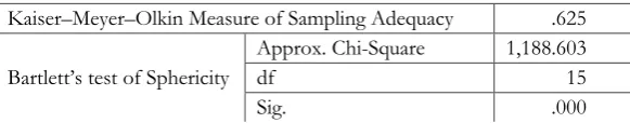
Since the ultimate aim of our analysis is to create homogeneous groups, the aggregate redundancy of individual layers was also examined. According to Sajtos–Mitev (2007), if the correlation between individual variables is too strong (above 0.9), their joint application leads to redundancy or distortion. Although no correlation of such strength was found, we had no information on the group of

variables. This is why the test/indicator expressing the suitability of the variables involved is used during the main component analysis. The KMO index has proved that the layers involved are suitable for the main component analysis, which means that redundancy exists but it has only a weak or moderate level (Sajtos–Mitev 2007, Füstös–Szalma 2009; Table 3).

In our opinion, the paired and aggregated correlations of the layers created with socio-economic content represent a versatile spatial structure and, therefore, enable us to describe the special features of the spatial structure in Central and Eastern Europe. Before that, though, we describe the spatial relations of the individual layers.

Table 3

Redundancy test of spatial structure layers

Kaiser–Meyer–Olkin Measure of Sampling Adequacy .625

Bartlett’s test of Sphericity

Approx. Chi-Square 1,188.603

df 15 Sig. .000

For this purpose, we have used bivariate global and local autocorrelation analyses. Table 4 contains Moran’s I for the bivariate global autocorrelation analyses. The purpose is to identify how one phenomenon influences the spatiality of another and to see the direction and strength of the spatial configuration resulting from their interaction13 _{(Anselin 2003). The layers in the first column of Table 4 represent}

spatially lagged variables ‘y’, while the layers in other columns always produce the corresponding variable ‘x’. The first figure (–0.297) expresses how the society layer influences the spatiality of the economy layer. The figure indicates negative neighbourhood assimilation for the two parameters.

Table 4

Bivariate global autocorrelation analyses of spatial structure layers (Moran’s I)

Society Concentration Infrastructure Innovation Settlement _pattern

Economy –.297 .064 .750 .424 .157

Society – .214 –0.350 –.157 .008

Concentration – .087 .053 .037

Infrastructure – .435 .297

Innovation – .105

The neighbourhood matrix is based on queen-1 contiguity. Pseudo-p 0.05; number of permutations: 999.

13 _{It is answered through Moran’s I. If I>–1/N–1 then the autocorrelation is positive; if I<–1/N–1 then it is}

Furthermore, the network and economy layers exhibit a tight parallel movement and clustering where Moran’s I equals 0.750. Negative neighbourhood assimilation was detected in three cases, while the remaining 12 cases show some level of positive autocorrelation.14 _{Nevertheless, the tight correlation detected formerly between the}

settlement structure and concentration layers (Table 2) is lost ‘in space’.

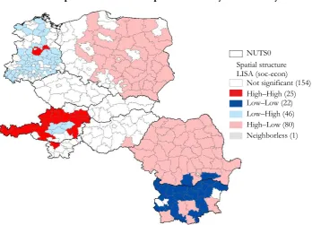
Figure 2

Local spatial autocorrelation pattern of society and economy

Accordingly, settlement structure does not generate any substantial spatial impact and only has an emanating impact on the individual socio-economic nodes.15 _{It is}

(also) probable, based on this correlation, that the spatial character of the level of socio-economic development takes the shape of a ‘bunch of grapes’.

The following Figures show two correlations of extreme values and describe their local pattern based on Local Moran’s I. The local pattern shows the spatial arrangement (high-high, low-low) of high values (hot spot) and low values (cold spot)

14 _{The sign and strength of the correlations are similar to those of the correlation coefficients.}

15 _{A methodological note should be made here. Both layers display a large number of outstanding values. This}

status is attributable to the applied indicator structure and the method of delimitation. (The impact of indicator structure is more marked in the case of the concentration layer as the use of density indicators facilitates the emergence of the above feature.) The logarithmisation of the applied indicators could have made it easier to identify spatial emanating impacts (due to the narrowing of the data series), but in this case the outstanding nature and the spatial dominance would have been eliminated for these subregions.

and the locations of the spatial units that significantly differ from each other (low–high, high–low).

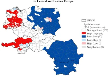
Figure 3

Spatial configuration of network and economy layers in Central and Eastern Europe

Although the negativity of neighbourhood assimilation is stronger between the network and society layers (Moran’s I= –0.350), we describe the joint spatial configuration of the two central layers (society and economy; Figure 2). This spatial arrangement shows the one-sided status of the two basic parameters in Central and Eastern Europe; the number of outlier subregions (LH, HL) exceeds, even separately, the extent of those in the clean (HH, LL) clusters. Adverse spatial relations (low society–low economy) occur mostly in the Bulgarian region and in two Romanian (cross-border) regions. The significant arrangement of high-high is present in only 26 subregions, and only Austria displays a continuous cluster. Apart from the HH clusters of Berlin and Potsdam in (the former) East Germany, almost the entire country area is a spatial outlier, and the adverse society layers are coupled with a fairly strong economy layer. The high society–low economy outlier cluster is fairly extensive: apart from the central and eastern subregions of Poland, it includes Romania and some subregions of Bulgaria. An example of spatially synergistic layers is shown in Figure 3. The east–west division of the network and economy layers is clearly visible, leading to significant hot spot and cold spot clusters. The majority of

East German and Austrian subregions is continuous HH, while LL groups exhibit a strong level of eastern determination. The number of outliers is small: only five regions ‘disturb’ the space of uniform clusters.

Results of cluster analysis

A cluster analysis was performed to typify the individual NUTS3 regions and to delimit the spatial units of various development stages that can be separated from each other.

At the start of the analysis, it is useful to recall that ‘the term of spatial structure should be used to denote designs that demonstrate the socio-economic features of geographic space in a selective, generalised, and simplified manner’ (Szabó–Farkas 2014). However, in our case, the large number of elements, the applied variables, and the issue of modifiable territorial units enabled and, moreover, forced us to display the versatile spatial structure. We have opted for the two-step cluster method because it: (i) eliminates the disadvantages of the K-means analysis suitable for handling a large number of elements (Lukovics–Kovács 2011), (ii) makes a proposal for the ideal number of clusters, and (iii) enables us to interpret groups of special characters (Sajtos–Mitev 2007). After several attempts, 21 was chosen as the number of clusters. This number was justified by the result of the Silhouette coefficient (0.4 means acceptable category) used for the statistical interpretation of consistency.

Table 5

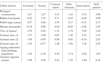
General features of city and urban clusters

Urban clusters Economy Society Concent-_{ration structure Innovation} Infra- _pattern Settl. Pentagon

cornerstones 1.67 1.27 5.15 1.43 0.75 3.98 Balkan focal point 0.22 1.21 9.71 –0.43 –0.28 4.98 Polish large centres 0.37 0.60 2.34 0.17 –0.31 2.73 Silesian metropolis –0.18 0.80 0.54 –0.05 –0.46 1.09 ‘City of science’ 1.95 0.25 1.31 1.78 9.29 1.22 German stars (1) 1.57 0.40 0.83 1.30 4.35 1.33 German stars (2) 1.49 –0.99 0.98 0.81 –0.10 2.25 German stars (3) 1.45 –0.17 1.28 1.96 1.36 2.29 Ageing subcentres

with declining

population 1.24 –1.50 0.30 1.14 0.42 1.05 Austrian regional

To avoid redundancy, the spatial structure of Central and Eastern Europe will be described in three parts. First, we describe the main focal points, cities and urban areas; then their spatial expansion and relevant groups (agglomerations and wider hinterlands); finally, the scarcely populated rural-peripheral clusters. Due to the differing delimitation (often by nation) of spatial units and the absence of a settlement network layer, the results need to be adjusted. Therefore, spatial typification was compared to the population-based categorisation of functional urban regions16

(Figure 4). In view of this (and our previous knowledge), it is stated in advance that the relevant metropolis regions can be detected and delimited with a good approximation. Additional spatial structure types (e.g. agglomerations, hinterlands, and scarcely populated rural areas) can also be identified. However, the specific nature of the delimitation represents a major obstacle for large functional urban areas with more than 250,000 inhabitants.

The groups of cities and urban areas shown as major socio-economic nodes result in a versatile structure; this is reinforced by the fact that these groups account for almost half of all clusters (Table 5). The first cluster, named Pentagon cornerstones,

includes cities located at the top of the settlement hierarchy: Berlin, Vienna, Prague, Budapest, and Warsaw. The most important socio-economic gravity points are ranked first in almost every layer: economy, concentration, and settlement structure are outstanding, while network and society provide one of the best results in urban areas. The only factor that lags behind is innovation: it shows the east-west division within the group as Budapest, Prague, and Warsaw produce only one-sixth or one-seventh of the patent indicators shown for Vienna and Berlin. Bucharest is the sole member of the cluster named Balkan focal point. Its socio-economic concentration, just like its settlement structure layer, is the highest in the region under review. Its economic dimension is significantly below the average, but this is true only for the static indicators. In fact, it has outstanding economic dynamics, the highest among the studied capital cities. The population retention layer is similarly positive in the capital city of Romania, although lags in the fields of infrastructure and innovation make Bucharest a one-sided urban pole. The next two clusters show national nature. The

Polish large centres such as Lodz, Cracow, Katowice, Poznan, Wroclaw, and the Tri-City (Gdansk-Sopot-Gdynia) emerge as substantial socio-economic gravity points in the Central and Eastern European space under review. Despite their large populations – indicated also by the outstanding values of the concentration and settlement

16 _{The urban function study of ESPON (2007) was used for this issue. In that study, the large functional urban}

structure layers – they perform poorly in terms of innovation and infrastructure, in comparison with other metropolis regions, and thus diminish their existing advantages. The Silesian metropolis covers most of the macroregion termed the ‘black hole’ by Gorzelak (1997). This cluster embodies the multi-centre agglomeration of Katowice, except for Moravia (Moravskoslezský kraj) in the Czech Republic. The Sofia region also joins the agglomeration, which is facilitated by similar settlement structure factors and the delimitation effort. Population retention is above the average in both clusters.

The next six clusters are located on the western side of the region under review, i.e. in (the former) East Germany and Austria. The cluster named City of science has only one member. The city of Jena represents the highest innovation potential in the region, coupled with a fairly strong economic position. Its role of socio-economic gravity point weakens in terms of population retention; ageing is a particular challenge for the city. The German stars cover German regions and the subregions of Graz and Bregenz. Their rank is based on economic output. The group of German stars (1)

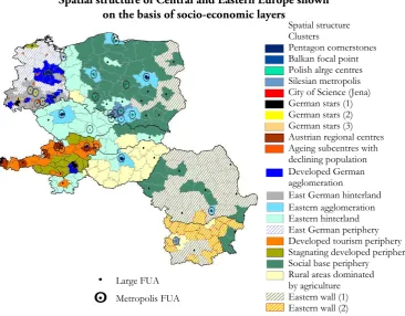
Figure 4

Spatial structure of Central and Eastern Europe shown on the basis of socio-economic layers

The Austrian regional centres represent the tertiary nodes of Austria (e.g. cross-border functional uban area of Salzburg, metropolis region of Linz-Wels, Innsbruck, etc.) or belong to such nodes (e.g. the southern agglomeration of Vienna). It is characterised with the most balanced layer structures; lagging in the case of concentration and settlement structure layers is attributable only to the delimitation effort.

Table 6

Average output of layers in the attraction zone regions

Emanating clusters Economy Society Concent-_{ration structure}Infra- _vation Inno- _pattern Settl.

Developed German

agglomerations 0.69 –0.42 –0.29 1.02 1.36 0.12 East German hinterland 0.60 –1.35 –0.31 1.13 –0.01 0.11 Eastern agglomeration –0.58 1.72 –0.09 0.02 –0.40 0.18 Eastern hinterland –0.04 0.73 –0.09 0.02 –0.34 –0.32

Spatial structure Clusters

Pentagon cornerstones Balkan focal point Polish alrge centres Silesian metropolis City of Science (Jena) German stars (1) German stars (2) German stars (3) Austrian regional centres Ageing subcentres with declining population Developed German agglomeration

East German hinterland Eastern agglomeration Eastern hinterland East German periphery Developed tourism periphery Stagnating developed periphery Social base periphery

Rural areas dominated by agriculture Eastern wall (1) Eastern wall (2)

.

.

o

Large FUA

The attraction zones are categorised along two distance dimensions: the ones closer to cities are called agglomerations and the larger ones located further away from cities are named hinterlands (Table 6). These attraction zones are divided in space as well. The differences come from the interaction between the layers. The east-west differences should be interpreted in terms of the economy, society, infrastructure, and innovation layers. The developed East German agglomerations refer to the attraction zones of Berlin, Dresden, Jena, Erfurt, and Graz. The economy, network, and innovation layers of the regions reinforce each other, but the society layer represents a strong deteriorating factor. However, the Eastern agglomerations excel in the field of population retention, while their other layers fail to reach the average of the region under review. The Eastern agglomerations represent the emanating impacts of such regional nodes and the Tri-City, Warsaw, Prague, Budapest, Bucharest, Cracow, Katowice, and Poznan. The East Germanhinterland and the Eastern hinterland cover an extensive zone of loose settlement structure beyond the agglomerating regions. Concentrated in the southern part of (the former) East Germany, the East German hinterland provides a background for agglomerations and metropolis FUAs. Moreover, the Eastern regions with an expanded attraction zone function as connection axes towards the West: Poland has a belt area along the German border, while the entire area of the Czech Republic, the western layers of Slovakia and Hungary, and the Slovenian layers of good network properties help the formation of these spaces. This spatial character facilitates the acceptance of the new banana structure.

The East German periphery is one of the most backward clusters in terms of the population layer; it is above the average economy and network layers are unable to improve the poor state of ageing, emigration, and unemployment. The categories of

developed tourism periphery and stagnating developed periphery are present mainly in Austria. Among the rural areas, the innovation layer is outstandingly reinforced – for the developed tourism peripherycluster type – by the economy, society, and network layers. This category is characterised by a high capacity for tourism. The subregions of Bratislava and Ljubljana are also part of the region; the awkward position is attributable partly to the delimitation effort.17 _{Although the level of concentration}

differs from that of other Austrian regions, the innovation, infrastructure, and society layers direct them into the same cluster. The units of stagnating developed periphery are found in Austria; their economic, network, and innovation potential exceeds that of similar cluster groups located in the east. The clusters named social base periphery and rural areas dominated by agriculture are similar, but the former has a vigorous population retention layer and the latter has a satisfactory economy layer. The remaining layers are significantly below the average. The peripheral regions are concentrated into two clusters named ‘eastern wall (1)’ and ‘eastern wall (2)’. These groups suffer from

17 _{Both capital cities were considered with their respective attraction zones. Their respective population figures}

multidimensional backlogs in terms of the economy, infrastructure, and innovation layers, which are the worst among the studied regions. The relatively more developed first group – encompassing Polish eastern subregions as well as Romanian and Bulgarian subregions – has a much stronger society layer, exceeding even that of rural areas dominated by agriculture (which comprise mostly Hungarian regions). The second category accommodates the least developed Romanian and Bulgarian regions, but the society layer does not exceed the average of the East German periphery (Table 7).

Table 7

Layer characteristics of rural and peripheral clusters

Emanating clusters Economy Society Concent-_{ration structure}Infra- _vation Inno- _pattern Settl.

East German periphery 0.60 –1.45 –0.49 0.58 –0.25 –0.67 Developed tourism

periphery 1.28 0.80 0.01 0.76 0.50 –0.20 Stagnating developed

periphery 0.69 0.00 –0.31 0.13 0.32 –0.56 Social base periphery –0.83 0.83 –0.21 –0.79 –0.47 –0.47 Rural areas dominated

by agriculture –0.47 –0.18 –0.33 –0.68 –0.42 –0.49 Eastern wall (1) –1.40 0.44 –0.38 –1.38 –0.50 –0.43 Eastern wall (2) –1.26 –0.84 –0.45 –1.38 –0.50 –0.69

Several large FUAs are found in the area covered by clusters named social base periphery and rural areas dominated by agriculture: on the eastern side of Poland, in the relatively more developed subregions of Romania, in the seaside regions of Bulgaria, and in Eastern Hungary. It is also evident that these smaller poles of regional level are unable to properly highlight their regional base from the rural space or to ascend to a higher category from the deep peripheries (e.g. see the cases of Bialystok, Lublin, Kielce, Brasov, Cluj Napoca, Constanta, and Varna). However, Iasi, Craiova, Galati, and Plovdiv are unable to make such upward progress due to their low socio-economic weight in the periphery of Central and Eastern Europe and to their (current) inability to improve their state of backwardness.

Summary

Our study aimed to demonstrate the spatial structure of Central and Eastern Europe. For this purpose, we employed and operationalised the spatial structure and then described the territorial characteristics of the region with the use of multivariate and spatial methods.

structure research work. The layers represent rather fragmented areas characterised by traditional differences (east-west, urban-rural) and other (nationwide) inequalities. The layers have versatile correlations and both synergistic and antagonistic mechanisms. In particular, the two most important layers (economy and society) do not show coherent parallel movements, which indicates serious problems in terms of future demographic processes. By employing the multivariate methodology, the relevant layers lead to a versatile spatial structure. As a result, it is difficult to perform the usual and straightforward categorisation using generalised figures. Therefore, we describe the main elements in three parts: cities/urban areas generating development, attraction zone regions, and rural/peripheral clusters. At the same time, our results also highlight the main transformation processes (demographics, innovation, and urbanisation) affecting the region. According to our analyses, developed areas that are either banana-shaped or shaped like a bunch of grapes (polycentric) can be found in the region. In the former case, the new banana shape seems to have a more solid base, and the mathematical-statistical methods have also identified a string of the western subregions of the Visegrád countries. However, the eastern wall covers a much larger area than in the former figures.

Since our study aimed to typify intermediate regions, i.e. areas considered peripheral from a European perspective (except for Austria), the study results should be interpreted within that framework. Although our study was intended to serve the purpose of identification and analysis, it may be used as a point of reference for the development aspects of European (cross-border, transnational, and inter-regional) territorial cooperation initiatives affecting the macroregions.

REFERENCES

ANSELIN,L. (2003): An Introduction to Spatial Autocorrelation Analysis with GeoDa Spatial Analysis Laboratory Department of Agricultural and Consumer Economics, University of Illinois, Urbana-Champaign.

ANSELIN,L. (2005): Exploring Spatial Data with GeoDaTM: A Workbook Center for Spatially Integrated Social Science, Spatial Analysis Laboratory Department of Geography University of Illinois, Urbana-Champaign.

BAJMÓCY, Z. – SZAKÁLNÉ KANÓ, I. (2009): Hazai kistérségek innovációs képességének elemzése Tér és Társadalom 23 (2): 45–68.

BRUNET,R. (1989): Les villes europeénnes: Rapport pour la DATAR Reclus, Montpellier. CSÉFALVAY,Z. (1999): Helyünk a nap alatt… Magyarország és Budapest a globalizáció korában

Kairosz Kiadó/Növekedéskutató, Győr.

EC (1999): European Spatial Development Perspective. Towards Balanced and Sustainable

Development of the Territory of the European Union Office for Official Publications of the European Communities, Luxembourg.

DOMMERGUES,P. (1992): The Strategies for International and Interregional Cooperation

Ekistics 59:352/353.

DUSEK,T. (2004): A területi elemzések alapjai Regionális Tudományi Tanulmányok 10., ELTE

TTK Regionális Földrajzi Tanszék, Budapest.

DUSEK,T.–KISS,J.P. (2008): A regionális GDP értelmezésének és használatának problémái

Területi Statisztika 48 (3): 264–280.

EC (2008): Green Paper on Territorial Cohesion. Turning territorial diversity into strength

Communication from the Commission to the Council, the European Parliament, the Committee of the Regions and the European Economic and Social Committee, Brussel.

EC (2010): Rural Development in the European Union Statistical and Economic Information Report 2010. Directorate-General for Agriculture and Rural Development, Brussel. EC (2011): Territorial Agenda of the European Union 2020. Towards an Inclusive, Smart, and Sustainable

Europe of Diverse Regions http://www.terport.hu/webfm_send/2291 (Downloaded: 12.10.2012).

DIJKSTRA,L.–POELMAN,H. (2011): Regional typologies: a compilation Regional Focus nr.

01/2011.

EC (2014): Population ageing in Europe Facts, implications and policies Directorate-General for Research and Innovation, Brussel.

EGRI, Z. – LITAUSZKY, B. (2012): Térszerkezeti sajátosságok Közép-Kelet-Európában

http://www.mrtt.hu/vandorgyulesek/2012/2/egri.ppt (Downloaded: 20.11.2015). ESPON (2005): Potentials for polycentric development in Europe ESPON 1.1.1. Project. ESPON

Coordination Unit, Luxembourg.

ESPON (2006): Urban-rural relations in Europe. ESPON 1.1.2. Final Report. ESPON Coordination Unit, Luxembourg.

ESPON (2007a): ESPON project 4.1.3 Feasibility study on monitoring territorial development based on ESPON key indicators ESPON Coordination Unit, Luxembourg.

ESPON (2007b): Study on Urban Functions ESPON 1.4.3 Final Report, ESPON Coordinate Unit, Luxembourg.

ESPON (2010): Metropolitan macroregions in Europe: from economic landscapes to metropolitan networks (Cities and their Hinterlands) FOCI Future Orientations for Cities Final Scientific Report, ESPON Coordinate Unit, Luxembourg.

ESPON (2012a): EDORA European Development Opportunities for Rural Areas Final Report, ESPON Coordination Unit, Luxembourg.

ESPON (2012b): SGPTD Second Tier Cities and Territorial Development in Europe: Performance, Policies and Prospects Final Report, ESPON Coordination Unit, Luxembourg.

ESPON (2014): ET2050 Territorial Scenarios and Visions for Europe Final Report, ESPON Coordination Unit, Luxembourg.

FÜSTÖS, L. (2009): A sokváltozós adatelemzés módszerei In.: Füstös L. – Szalma I. (ed.):

Módszertani füzetek 2009/1. MTA Szociológiai Kutatóintézete Társadalomtudományi Elemzések Akadémiai Műhelye (TEAM), Budapest.

GORZELAK, G. (1997): Regional Development and Planning in East Central Europe In:

KEUNE,M. (Ed.): Regional Development and Employment Policy: Lessons from Central and

GORZELAK,G. (2001): Regional Development in Central Europe and European Integration

Informationen zur Raumentwicklung Heft (11/12): 743–749.

GORZELAK,G. (2006): Main Processes of Regional Development in Central and Eastern Europe after

1990. Regional Diversity and Local Development in Central and Eastern Europe Conference paper. http://www.oecd.org/dataoecd/58/41/37778478.pdf (Downloaded: 20.11. 2015).

HALL,P. (1992): Urban and Regional planning Routledge, London.

HORVÁTH, GY. (2013): A német Mezzogiorno? A keletnémet regionális fejlődés az

újraegyesítés után Területi Statisztika 53: (5) 492–514.

KINCSES,Á.–NAGY,Z.–TÓTH,G. (2013a): Európa térszerkezete különböző matematikai

modellek tükrében, I. rész Területi Statisztika 53 (2): 148–156.

KINCSES,Á.-NAGY,Z.-TÓTH,G. (2013b): Európa térszerkezete különböző matematikai

modellek tükrében, II. rész Területi Statisztika 53 (3): 237–252.

KUNZMANN,K.R.–WEGENER,M. (1991): The pattern of Urbanization in Western Europe

Ekistics 58: 350–351.

LEIBENATH,M.–HAHN,A.–KNIPPSCHILD,R. (2007): Der „Mitteleuropäische Kristall“ –

zwischen „Blauer Banane“ und „osteuropäischem Pentagon“. Perspektiven der neuen zwischenstaatlichen deutsch-tschechischen Arbeitsgruppe für Raumentwicklung

Angewandte Geographie 31 (1): 36–40.

LENGYEL,I.–RECHNITZER,J. (2004): Regionális gazdaságtan Dialóg Campus Kiadó,

Budapest-Pécs.

LENGYEL, I. (2012): Regionális növekedés, fejlődés, területi tőke és versenyképesség In.:

BAJMÓCY, Z. – LENGYEL, I. – MÁLOVICS, GY. (ed.): Regionális innovációs képesség,

versenyképesség és fenntarthatóság pp. 151–174., JATEPress, Szeged.

LENGYEL,I. (2003): Verseny és területi fejlődés: térségek versenyképessége Magyarországon JATEPress,

Szeged.

LUKOVICS,M.–KOVÁCS,P. (2011): A magyar kistérségek versenyképessége Területi Statisztika

51 (1): 52–71.

LUX,G. (2012): A gazdaság szerepe a városi térségek fejlesztésében: A globális kihívásoktól a

fejlesztéspolitikáig In.: SOMLYÓDYNÉ PFEIL,E. (ed.): Az agglomerációk intézményesítésének

sajátos kérdései: Három magyar nagyvárosi térség az átalakuló térben pp. 67–89., Publikon Kiadó, Pécs.

NEMES NAGY,J.–TAGAI,G. (2009): Területi egyenlőtlenségek, térszerkezeti determinációk

Területi Statisztika 49 (2): 152–169.

OECD (2011): Invention and Transfer of Environmental Technologies OECD Studies on Environmental Innovation, OECD Publishing, Washington.

OECD (2013): Regions and Innovation: Collaborating across Borders OECD Reviews of Regional Innovation, OECD Publishing, Washington.

PAQUÉ, K-H. (2009): The Transformation Policy in East Germany – A Partial Success Story

http://www.kas.de/upload/Publikationen/Panorama/2009/1/paque.pdf (Downloaded: 15.11.2014).

PORTER,M.E.–STERN,S. (2001): National Innovative Capacity Oxford University Press, New

RECHNITZER, J. – GROSZ, A. – HARDI, T.– KUNDI, V. – SURÁNYI, J. – SZÖRÉNYINÉ

KUKORELLI,I. (2008): A magyarországi Felső-Duna szakasz fejlesztési kérdései MTA RKK

NYUTI, Győr.

RECHNITZER,J.–SMAHÓ,M. (2011): Területi politika Akadémiai Kiadó, Budapest.

RECHNITZER, J. (2013): Adalékok Kelet-Közép-Európa térszerkezetének felrajzolására

Geopolitika a XXI. században 3 (4): 35–52.

SAJTOS,L.-MITEV,A. (2007): SPSS kutatási és adatelemzési kézikönyv Alinea Kiadó, Budapest.

SIC! (2006): Sustrain implement corridor. Long factbook.

http://195.230.172.167/cms_sic/upload/pdf/061010_SIC_LongFactbook.pdf (Downloaded: 12.10.2012).

SIMAI,M. (2014): A térszerkezet és a geoökonómia Tér és Társadalom 28 (1): 25–39.

SMAHÓ,M. (2011): A tudás és a regionális fejlődés összefüggései Doktori értekezés. Széchenyi István

Egyetem Multidiszciplináris Társadalomtudományi Doktori Iskola, Győr.

SZABÓ,P.–FARKAS,M. (2014): Kelet-Közép-Európa térszerkezeti képe Tér és Társadalom 28

(2): 67–86.

SZABÓ,P.(2009): Európa térszerkezet különböző szemléletek tükrében Földrajzi Közlemények

133 (2): 121–134.

STIMSON,R. – STOUGH,R.R.–NIJKAMP,P. (2011): Endogenous regional development Edward

Elgar, Cheltenham.

TÓTH,G. (2013): Bevezetés a területi elemzések módszertanába Miskolci Egyetem, Miskolc.

TÓTH,SZ. (2003): A régiók Európája Korunk 14 (1): 97–106.

VAN DER MEER,L. (1998): The Red Octopus In: BLAAS,W. (ed.) A new perspective for European

spatial development policies pp. 9–26., Avebury, Aldershot.

ANNEX

Spatial model of Central and Eastern Europe in the 1990s

Source: Szabó–Farkas (2014) based on Rechnitzer–Smahó (2011).

Internationally significant city Potentially internationally significant city

Transnational significant city Regional centre with international significance

Current development zone Potential development zone

North-South future cooperation region with development cooperation European transportation corridor

Potential multiregional cooperation

Tourism region Peripherial region

Multi-regional cooperation

Development core area

Traditional industry area

Old and New banana in Europe

The European Macroregions

Source: Leibenath et al. (2007).

Expanded Czech–German space West European Pentagon Central European Pentagon Blue Banana

Sun Belt Region European macroregions