What Are the Carbon Emissions Elasticities for Income and Population? Bridging STIRPAT and EKC via robust heterogeneous panel estimates

What Are the Carbon Emissions

Elasticities for Income and Population?

Bridging STIRPAT and EKC via robust

heterogeneous panel estimates

Liddle, Brantley

2015

Online at

https://mpra.ub.uni-muenchen.de/61304/

What Are the Carbon Emissions Elasticities for Income and Population? Bridging STIRPAT and EKC via robust heterogeneous panel estimates

Brantley Liddle

Asia Pacific Energy Research Centre Tokyo, Japan

Centre for Strategic Economic Studies, Victoria University Melbourne, Australia

btliddle@alum.mit.edu

ABSTRACT

Knowledge of the carbon emissions elasticities of income and population is important both for climate change policy/negotiations and for generating projections of carbon emissions. However, previous estimations of these elasticities using the well-known STIRPAT framework have produced such wide-ranging estimates that they add little insight. This paper presents estimates of the STIRPAT model that address that shortcoming, as well as the issues of cross-sectional dependence, heterogeneity, and the nonlinear transformation of a potentially integrated variable, i.e., income. Among the findings are that the carbon emissions elasticity of income is highly robust; and that the income elasticity for OECD countries is less than one, and likely less than the non-OECD country income elasticity, which is not significantly different from one. By contrast, the carbon emissions elasticity of population is not robust; however, that elasticity is likely not statistically significantly different from one for either OECD or non-OECD countries. Lastly, the heterogeneous estimators were exploited to reject a Carbon Kuznets Curve: while the country-specific income elasticities declined over observed average income-levels, the trend line had a slight U-shape.

Keywords: Carbon Kuznets Curves; Kaya identity; population and environment; nonstationary panels; cross sectional dependence; nonlinearities in environment and development.

Acknowledgements

The Pesaran (2004) CD test, the Pesaran (2006) common correlated effects mean group

estimator, and the Eberhardt and Teal (2010) augmented mean group estimator were developed for STATA by Markus Eberhardt. The Pesaran (2007) panel unit root test was developed for STATA by Piotr Lewandowski. The final version benefited from comments by anonymous reviewers and the participants of a workshop organized by Brian O’Neill at the National Center for Atmospheric Research, Boulder, CO in 2012.

1. Introduction and background

Improved understanding of the carbon emissions elasticities of income and population is

important both for climate change policy/negotiations and for generating projections of

emissions. Indeed, the Kaya Identity—which treats total carbon emissions as a product of

population GDP per capita, energy use per unit of GDP, and carbon emissions per unit of energy

consumed—plays a key role in the Intergovernmental Panel on Climate Change estimates of

future carbon emissions (Kaya 1990). This paper uses the Kaya/STIRPAT framework to

determine what are the carbon emissions elasticities for income and population and whether

those elasticities differ across development/income or population levels. The paper considers two

econometric estimation methods—the Pesaran (2006) common correlated effects mean group

estimator (CMG) and the Eberhardt and Teal (2010) augmented mean group estimator (AMG)—

that address important (but often neglected) time-series cross-section (TSCS) issues:

nonstationarity, cross-sectional dependence, and heterogeneity. Furthermore, the paper addresses

an additional important empirical issue particular to environment-development research—the

nonlinear transformation of potentially integrated variables (see Wagner 2008 and Stern 2010 for

previous treatments).

In addition to providing a critique of STIRPAT (Stochastic Impacts by Regression on

Population, Affluence, and Technology) modeling, this paper bridges the STIRPAT literature

with other socio-economic models of environmental impact that place the dependent variable in

per capita terms—e.g., Environmental Kuznets Curve (EKC). That bridge is established by

demonstrating that best practice suggests assuming the population elasticity is unity since

estimations of the carbon emissions elasticity of population are: (i) not robust, (ii) typically not

either income or population size. By contrast, the estimations reported here demonstrate that the

carbon emissions elasticity of income are: (i) highly robust, (ii) significantly less than one (but

positive) for OECD countries, and (iii) significantly larger for non-OECD countries than for

OECD countries (but not different from significantly one for non-OECD countries). Also, the

heterogeneous nature of the estimators considered was exploited to show that those income

elasticities fall with average income but do not become negative.

Much discussion and research on national differences in the influence of population and

of development/consumption (typically represented by GDP per capita) on key environmental

indicators like carbon emissions are based on: (i) the IPAT equation (introduced by Ehrlich and

Holdren 1971 and Commoner et al. 1971)—which decomposed aggregate environmental impacts

(I) into contributions from population growth (P), growth in per capita income or consumption

(as measures of affluence, A), and changes in technology (T); and (ii) its econometric progeny,

coined STIRPAT by Dietz and Rosa (1997). In general, the STIRPAT model is:

it d it c it b it

it aP A T e

I = (1)

where the subscript i denotes cross-sectional units (e.g., countries), t denotes time period, the

constant a and exponents b, c, and d are to be estimated, and e is the residual error term.

Since Equation 1 is linear in log form, the estimated exponents can be thought of as

elasticities (i.e., they reflect how much a percentage change in an independent variable causes a

percentage change in the dependent variable.) Also, the T term is often treated like an intensity of

use variable and sometimes modeled as a combination of log-linear factors. Furthermore,

Equation 1 is no longer an accounting identity whose right and left side dimensions must

balance, but a potentially flexible framework for testing hypotheses—such as (i) whether

marginal impact on the environment; and (iii) whether population’s elasticity is different from

unity, i.e., whether population or impact/emissions grow faster.

That last hypothesis is particularly important to test since, if population’s elasticity is one,

then population as an independent variable could be removed (from Equation 1) via division.

Hence, the dependent variable would be in per capita terms, and the STIRPAT model would

collapse into a framework similar to those used in nearly all other socio-economic investigations

of emissions/energy consumption, e.g., the EKC literature (Dinda 2004 and Stern 2004 provided

somewhat early reviews of this vast literature). The EKC literature seeks to determine whether

there is an inverted-U relationship between GDP per capita and emissions or other environmental

impact measure per capita. When the dependent variable is carbon emissions per capita, these

studies are sometimes referred to as estimating Carbon Kuznets Curves or CKC (Iwata et al.

2011 and 2012 are recent examples). The EKC/CKC literature posits that pollution first rises

with income and then falls after some threshold level of income/development is reached (Liddle

2013a presents a detailed review/explanation of the differences between the STIRPAT model

and other socio-economic models/literatures like the EKC and energy-GDP causality).

Empirical studies of the EKC/CKC typically take the following form:

ln / = + + ln + (ln ) + ln( ) + (2)

where a and g are the cross-sectional and time fixed effects, respectively, and Z is a vector of other drivers that is sometimes considered—similar to T in Equation 1. Hence, the primary

difference between the STIRPAT and EKC/CKC frameworks (i.e., between Equations 1 and 2)

is that the EKC effectively assumes that population’s elasticity is unity and correspondingly

converts the dependent variable into per capita terms. An EKC/CKC between emissions per

while the coefficient is statistically significant and negative. (Liddle 2004 and Richmand and

Kaufmann 2006 argued that if the corresponding turning point occurs outside the sample range,

the estimated relationship is more like a semi-log or log-log one than an inverted-U; however,

many EKC analyses do not even report implied turning points, and so it is not clear how widely

accepted this interpretation is.)

More recently, a literature has emerged that attempts to bridge the CKC and energy-GDP

causality literatures by adding energy consumption as an explanatory variable to the typical CKC

model (e.g., Apergis and Payne 2009 and 2010; and Lean and Smyth 2010). Itkonen (2012)

critiqued this new literature and called its model emissions-energy-output (EEO). Itkonen

described the EEO model (for the single country case) as:

= + + + + (3)

where C is carbon dioxide emissions per capita, E is total energy use per capita, Y is real GDP

per capita, and u is an error term.

In addition to addressing nonstationarity, cross-sectional dependence, and heterogeneity,

the current paper provides a bridge between the STIRPAT and EKC/CKC/EEO literatures. That

bridge is constructed by determining whether population’s elasticity should be considered to be

different from unity, and by exploiting heterogeneous estimators to address possible

nonlinearities—thus, avoiding the statistical pitfall of nonlinear transformations of nonstationary

variables. Further, the lessons learned here about econometric estimation methods should be

useful to other modelers—11 of the 17 STIRPAT studies listed in Table 1 were published in

2010 or later. (Yet, there are many more, recent studies applying the STIRPAT framework that

are not listed in Table 1 because they considered different dependent variables, were not

the EKC/CKC/EEO models continue to be popular—Itkonen (2012) cited 16 EEO studies, of

which only two were published prior to 2009 (and, for example, Baek and Kim 2013; Saboori

and Sulaiman 2013 used the EEO model but were published after Itkonen).

2. Brief literature review and important empirical issues

The cross-national, inter-temporal studies applying the STIRPAT formulation to carbon

emissions typically found that both population and income/affluence are significant drivers (see

Table 1). Furthermore, most studies have found that population has a greater environmental

impact (i.e., elasticity) than affluence (e.g., Dietz and Rosa 1997; Shi 2003; Cole and Neumayer

2004; Martinez-Zarzoso et al. 2007; Liddle and Lung 2010). However, these STIRPAT analyses

have produced a wide range of income and population elasticity estimates—from 0.15 to 2.50 for

income and from 0.69 to 2.75 (with several statistically insignificant findings) for population.

Moreover, in answering the question, “is population’s elasticity significantly different from one,”

those studies have produced highly inconsistent results. For example, Cole and Neumayer (2004)

found population’s elasticity to be statistically indistinguishable from unity (thus, a 1% increase

in population caused an approximate 1% increase in emissions). By contrast Shi (2003)

estimated a particularly high elasticity for population—between 1.4 and 1.6 for all countries

samples; when Shi separated countries by income groups, the elasticity for high income countries

was 0.8, whereas the elasticity for middle and low income countries ranged from 1.4 to 2.0.

Similarly, Martinez-Zarzoso et al. (2007) estimated a statistically insignificant population

elasticity for old EU members, but an elasticity of 2.7 for recent EU accession countries. Table 1

suggests several reasons for this substantial variation: different datasets, different additional

variables, and, perhaps most important, whether and how nonstationarity and heterogeneity were

Table 1

2.1 Stationarity

Most variables used in STIRPAT analyses are stock (population) or stock-related

variables (GDP, emissions, and energy consumption, which are influenced by stocks like

population and physical capital); as such, those variables are highly trending and quite possibly

nonstationary—i.e., their mean, variance, and/or covariance with other variables changes over

time. For example, in the energy economics literature a number of researchers have found

variables like GDP per capita, energy consumption, and carbon emissions to be nonstationary in

levels but stationary in first differences for panels of developed and developing countries (e.g.,

Apergis and Payne 2009 and 2010; Lean and Smyth 2010; and Liddle 2013b).

When ordinary least squares (OLS) regressions are performed on series (or on

time-series cross-section) variables that are not stationary, then measures like R-squared and

t-statistics are unreliable, and there is a serious risk of the estimated relationships being spurious

(Kao 1999; Beck 2008). Yet, several STIRPAT studies that employ annual times-series

cross-section data have been unconcerned with the stationarity issue (see Table 1). (Indeed, Cole and

Neumayer 2004 hypothesized that the much higher elasticity estimated in Shi 2003 may be

spurious because of that paper’s use of untreated, nonstationary data.) Most of the STIRPAT

studies that have addressed stationarity in their data have done so via first differences (e.g., Cole

and Neumayer 2004; and Martinez-Zarzoso et al. 2007). Although first-differencing often

transforms nonstationary variables into stationary ones, first-differencing means that the model is

a short-run (rather than a long-run) model, and that the estimated coefficients reflect how

percentage changes in the growth rate of independent variables relate to percentage changes in

al. 2011 and 2012) and the broader GDP literature (which includes both EEO and

energy-GDP causality analyses) have estimated long run elasticities using methods that address

nonstationarity.

2.2 Cross-sectional dependence

Recently, the TSCS econometric theory literature has turned its attention toward testing

for and correcting cross-sectional dependence. For variables like GDP per capita and carbon

emissions, cross-sectional dependence is expected because of, for example, regional and

macroeconomic linkages that manifest themselves through (i) common global shocks, like the oil

crises in the 1970s or the global financial crisis from 2007 onwards; (ii) shared institutions like

the World Trade Organization, International Monetary Fund, or Kyoto Protocol; or (iii) local

spillover effects between countries or regions. These shocks or institutions can be thought of as

omitted variables, and are likely to be correlated with the regressors (Sarafidis and Wansbeek

2012). When the errors of panel regressions are cross-sectionally correlated, standard estimation

methods can produce inconsistent parameter estimates and incorrect inferences (Kapetanios et al.

2011). Yet, Sadorsky (2014) is the only other STIRPAT analysis that employs methods to

estimate long-run coefficients that are demonstrated to be robust to cross-sectional correlation,

and perhaps only Wagner (2008), Stern (2010), and Mazzanti and Musolesi (2013) have

performed such estimations in the panel EKC/CKC literature. Indeed, even the broader

energy-GDP literature typically has not estimated panel elasticities robust to cross-sectional correlation;

known exceptions are Belke et al. (2011), Liddle (2013b), Sadorsky (2013), and Liddle and Lung

2.3 Heterogeneity and nonlinearities

Heterogeneity, when considered, is typically addressed by splitting the panel along

income lines (e.g., Poumanyvong and Kaneko 2010); indeed, nearly all STIRPAT studies have

employed pooled estimators that otherwise assume the population-environment (or STIRPAT)

relationship is the same for each country analyzed. By contrast, the estimators used in Liddle

(2011 and 2013a) allow for a high degree of heterogeneity in the panel(s); hence, besides

producing consistent point estimates of the panel sample means, those estimators provide

country-specific estimates of all parameters accompanied by efficient standard normal errors.

Indeed, Liddle (2011) demonstrated a substantial variation in individual STIRPAT elasticity

estimations among OECD countries. And if one mistakenly assumes that the parameters are

homogeneous (when the true coefficients of a dynamic panel in fact are heterogeneous), then all

of the parameter estimates of the panel will be inconsistent (Pesaran and Smith 1995). The recent

CKC and EEO literatures are mixed regarding the use of long run heterogeneous estimators; e.g.,

Apergis and Payne (2009 and 2010) and Lean and Smyth (2010) allowed for heterogeneity,

while Iwata et al. (2011 and 2012) did not.

The EKC/CKC literature has hypothesized that the emissions-income relationship may

vary across income/development levels; similarly, the environmental/emissions impact of

population could change with either development (income) level or population size. That

question of nonlinear relationships often is addressed by including a squared term in regressions

and testing whether the coefficient for that squared term is negative and statistically significant.

However, if the variables of interest (e.g., GDP per capita, population) are nonstationary or I(1)

variables—as previous studies reported above as well as the tests reported below indicate they

variables could be spurious, and their significance tests invalid (Bradford et al. 2005). (A

variable is said to be integrated of order d, written I(d), if it must be differenced d times to be

made stationary. Thus, a stationary variable is integrated of order zero, i.e., I(0), and a variable

that must be differenced once to become stationary is integrated of order one or I(1).)

Wagner (2008) further argued that all previous EKC analyses that used panel data failed

to account for both cross-sectional dependence and the nonlinear transformation of integrated

GDP per capita. Relatedly, Itkonen (2012) argued that the nonlinearity of the CKC model

(irrespective of order of integration issues) is incompatible with the vector autoregression (VAR)

models used in the EEO literature; and hence, VAR models with such transformed regressors

produce unreliable estimates.

Also, that polynomial model/regression does not allow for the possibility that elasticities

are significantly different across development levels but still positive. Liddle (2013a) motivated

the use of income-based panels to avoid this nonlinear transformation of a nonstationary variable

while determining whether income effects differed across development/income levels. As will be

discussed further below, we will exploit the heterogeneous estimators to determine whether GDP

per capita’s or population’s impact is nonlinear.

3. Model, data, and methods

In addition to the usual independent variables of population and income/affluence, we

consider two technology or intensity-type variables that are variations on two variables from the

Kaya Identity: the carbon intensity of energy and the energy intensity of GDP. As a proxy for the

carbon intensity of energy, we consider the share of primary energy consumption from non-fossil

(2010). Rather than include the aggregate energy-GDP ratio (or energy intensity), we consider,

as did Liddle and Lung (2010), a measure of industrial energy intensity.

National, aggregate carbon emissions are calculated from national, aggregate energy

consumption; thus, for countries with carbon intensive energy sources, aggregate carbon

emissions and aggregate energy intensity run the risk of being highly correlated by construction,

and thus, inappropriate for regression analysis. By contrast, this measure of industrial energy

intensity—constructed as industrial energy consumption (from the International Energy Agency)

divided by industrial output (in GDP terms)—is not highly correlated with national carbon

emissions (see Table 2, which shows such correlations). In addition, industrial energy intensity

measures both the size of industrial activity and the composition of such activity (i.e., the

presence of particularly energy intensive sectors like iron and steel and aluminum smelting);

thus, it is preferable to measures of economic structure, like manufacturing’s or industry’s share

of GDP. Industry is a diverse sector with respect to energy intensity, as it ranges from iron and

steel and chemicals to textiles and the manufacturing of computing, medical, precision, and

optical instruments. Some of those more technology-intensive manufacturing sectors may be less

energy intense than some service sectors like transport, hospitality, and hospitals. Also, as Liddle

and Lung (2010) argued, just because the share of economic activity from manufacturing or

industry has declined does not mean the level of such activity has fallen; and it is the level of

activity that should influence the level of aggregate emissions.

Industrial energy intensity (IEI) and the share of primary energy consumption from

non-fossil fuels (Sh nff) are drawn from the International Energy Agency (IEA). Population (P),

carbon emissions (I), and real GDP per capita (A, which is converted to USD via purchasing

over 1971-2011 from 26 OECD countries and 54 non-OECD countries. Every country with data

beginning in at least 1985 was included (variables relating to industry output and industry energy

consumption are what most restricted dataset coverage), and, according to World Bank data, the

included countries accounted for 86% and 91% of 2011 world population and GDP, respectively,

and 80% of 2010 world carbon dioxide emissions. (Appendix A lists the countries considered.)

Summary statistics and correlations are displayed in Table 2.

Table 2

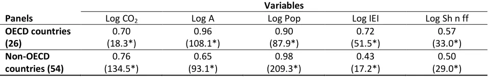
Table 3 displays the results of the Pesaran (2004) CD test, which employs the correlation

coefficients between the time-series for each panel member. The null hypothesis of

cross-sectional independence is rejected for each variable and for both panels; moreover, several of the

absolute value mean correlation coefficients are very high. The Pesaran (2007) panel unit root

test (CIPS) allows for cross-sectional dependence to be caused by a single (unobserved) common

factor, and that test is valid for both unbalanced panels and panels in which the cross-sectional

and time dimensions are of the same order of magnitude; the results of that test suggest that

carbon emissions, affluence/income, industrial energy intensity, and population are I(1). (Unit

root test results are discussed in Appendix B and shown in accompanying tables.)

Table 3

Two OLS-based, heterogeneous or mean group type estimators are considered; they first

estimate each group/cross-section specific regression and then average the estimated coefficients

across the groups/cross-sections (standard errors are constructed nonparametrically as described

in Pesaran and Smith 1995). Hence, the equation analyzed is:

it it i

it i

it i it i i

it c P d A e IEI f Shnff

I =a + ln + ln + ln + ln +e

where subscripts it denote the ith cross-section and tth time period. Again, the slope coefficients

(ci, di, ei, and di) are heterogeneous, and the constant arepresents country-specific effects.

Both mean group estimators were specifically designed to address both stationarity and

cross-sectional dependence/correlation in TSCS models: the Pesaran (2006) common correlated

effects mean group estimator (CMG), and augmented mean group (AMG) estimator by

Eberhardt and Teal (2010). The CMG estimator accounts for the presence of unobserved

common factors by including in the regression cross-sectional averages of the dependent and

independent variables. The AMG estimator accounts for cross-sectional dependence by including

in the regression a common dynamic process—which is extracted from year dummy coefficients

of a pooled regression in first differences. Both the CMG and AMG estimators are robust to

nonstationary variables, whether cointegrated or not (Eberhardt and Teal 2010); thus, arguably,

they do not require the pre-testing (neither to determine the existence of cointegration nor to

confirm that all variables are of the same order of integration) that other heterogeneous,

nonstationary panel estimators like Fully Modified OLS and Dynamic OLS require. Also, both

the CMG and AMG estimators are robust to serial correlation (Pesaran 2006; Eberhardt and Teal

2010, respectively); and CMG-type estimators are robust to structural breaks (Kapetanios et al.

2011).

For diagnostics we run the Pesaran (2004) CD test on the residuals and report the mean

absolute correlation coefficient to determine/measure the extent of cross-sectional dependence,

and the Pesaran (2007) CIPS test to demonstrate that the residuals are I(0). Appendix Table C.1

displays elasticity results (and diagnostics) from several other popular TSCS estimators. The

diagnostic results displayed in Table C.1 suggest that the CMG and AMG estimators are

(For discussion of several of the estimators in Appendix C and their results see the working

paper version, Liddle 2012.) Lastly, the CMG and AMG estimators allow the inclusion of

individual, country-specific time trends. The decision on whether to include such trends was

based on two factors: (i) the share of cross-sections for which such trends were statistically

significant at the 5% level; and (ii) whether the inclusion of such trends substantially improved

the panel cross-sectional dependence diagnostics. However, the full regression results (each

estimation with and without individual time trends) are contained in a supplemental file.

4. Results and discussion

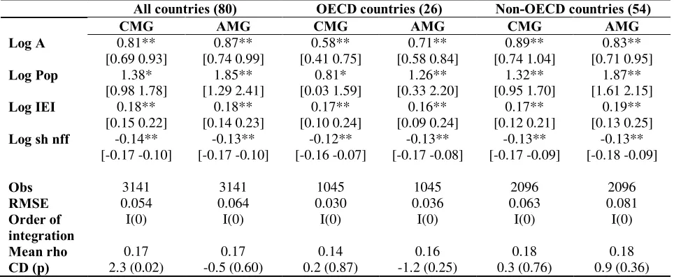
Table 4 displays the regression results from the two heterogeneous panel estimators

(CMG and AMG) for an all countries panel and with the sample divided between the 26 OECD

countries and the 54 non-OECD countries. For all three sets of regressions all the coefficients

have the expected signs and are statistically significant. In addition, the diagnostics are good: the

residuals always are stationary, and either cross-sectional independence in the residuals cannot

be rejected or cross-sectional dependence is mitigated (small mean correlation coefficients).

The all countries panel results suggest that population’s elasticity may be significantly

larger than that of income’s and significantly greater than unity. Yet, dividing the sample into

two panels may be justified since, in comparing the confidence intervals for the two panels

(OECD vs. non-OECD countries), the income elasticity for carbon emissions, when estimated

via CMG, is greater for non-OECD countries than for OECD countries—evidence of an income

saturation effect. (For the other three variables, the elasticities are not statistically significantly

Table 4

For OECD countries, the elasticity for income is significantly less than one, whereas, the

elasticity for population is not different from one at the 5% level of statistical significance. For

non-OECD countries, the long-run elasticity for income is not significantly different from one

for the CMG estimator. The elasticity for population is, as for the all countries panel, greater than

one on average; yet, only for the AMG estimator is the elasticity for population statistically

significantly greater than one or possibly statistically significantly greater than the elasticity for

income.

4.1 Sensitivity/robustness over time

To test whether the elasticities for affluence and population are robust over time, the two

estimators (CMG and AMG) are performed on 12 different time spans for both of the panels

(OECD and non-OECD countries)—a total of 48 regressions (see Appendix D for the time spans

considered). To avoid the problem of the panels differing substantially across time spans, only

countries with data beginning in 1971 were considered. The elasticity estimations for income and

population from those 48 panel regressions are displayed in Appendix D; we summarize those

results here. The panel elasticities for affluence were highly robust: the average panel coefficient

(from the different time-span regressions) was similar to that shown in Table 4; the coefficients

were always statistically significant; and for the OECD panel, the affluence coefficient was

statistically different (smaller) than unity in all but three of the 24 regressions—by contrast, for

non-OECD countries, the coefficient was different from unity in only six of 24 regressions.

On the other hand, the population elasticity was not robust. For the CMG estimator (and

both the OECD and non-OECD panels), the population elasticity was statistically significant in

elasticity was statistically significant in 21 of them; however, it was never statistically different

from unity for the OECD panel and was only statistically significantly different from unity

(larger) in three of 12 regressions for the non-OECD panel. (The sensitivity analysis—displayed

in Appendix D—revealed no evidence that the size, significance, or sign of the population

elasticity may have changed over-time, e.g., from 1970-1990 to 1990-2006.)

4.2 Nonlinearities in population and income elasticities

In addition to the possibility that the income and population elasticities could be different

at different levels of development (i.e., in OECD vs. non-OECD countries), these elasticities

could change as the level of income or population changes. Thus, we consider whether the

individual country income/population elasticity estimates vary according to the level of

income/population by plotting those elasticity estimates against the individual country average

income/population for the whole sample period (rather than by including in the regression

equation nonlinear transformations of these I(1) variables).

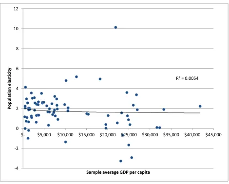
4.2.1 Nonlinearities in population elasticities

Figure 1 shows the country-specific population elasticities (from the AMG estimator)

plotted against the individual country average GDP per capita for the sample period (for all

countries). (The results from the CMG estimator were essentially the same.) Here, there appears

no relationship (R-squared is 0.005)—the population elasticities do not vary meaningfully

according to income.

Figure 1

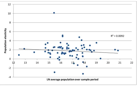
Similarly, there was no relationship between the individual country population elasticity

and country average population size. Figure 2 displays the country-specific population

countries). The resulting trend line (also shown in the figure) is (nearly) horizontal, and the

R-squared is less than 0.01.

Figure 2

4.2.2 Carbon emissions per capita estimates and nonlinearities in income elasticities

It seems reasonable to estimate a model with carbon emissions per capita as the

dependent variable (and thus no independent population variable) given (i) what we have just

shown—that the population elasticity does not vary meaningfully according to income level or

population size; (ii) the previous discussion of the sensitivity results—that the population

elasticity was significantly different from unity in only about 10% of the regressions; and (iii) the

O’Neill et al. (2012) argument that, “… if all other influences on emissions are controlled for,

and indirect effects of population on emissions through other variables are excluded, then

population can only act as a scale factor[,] and its elasticity should therefore be 1.” Furthermore,

converting the dependent variable into per capita terms makes the transformed model

comparable to the models used in nearly all other socio-economic investigations of

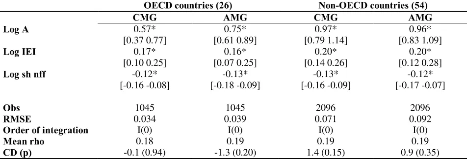
emissions/energy consumption—e.g., EKC/CKC and EEO models. Table 5 displays the results

of such carbon emissions per capita estimates.

Table 5

All of the diagnostics are good: the residuals always are stationary, and cross-sectional

independence in the residuals can never be rejected. Also, the estimates of the remaining

variables are very similar to those estimates shown in Table 4. Again, there is evidence of an

income saturation effect, and thus, a justification to separate dataset into (at least) two panels

(OECD vs. non-OECD countries). Indeed, in comparing the confidence intervals for the two

for carbon emissions is greater for non-OECD countries than for OECD countries (although the

AMG estimations are different only at the 10% significance level).

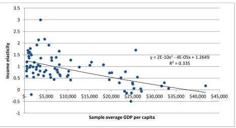
Lastly, Figure 3 shows the country-specific income elasticity estimates (from the model

with carbon emissions in per capita terms) plotted against the individual country average GDP

per capita for the sample period (for all countries). (The AMG estimator was used, and again, the

results from the CMG estimation were essentially the same.) The figure also indicates the

quadratic trend line (which has an R-squared of 0.34). The income elasticities fell throughout the

average income range. While two countries (Belgium and Sweden) estimated statistically

significant negative elasticities, there is no evidence that a panel income elasticity would become

negative—indeed, the trend line has a slight U-shaped pattern; thus, a CKC, where carbon

emissions would eventually decline with income, is rejected. (When the CMG estimator was

used, no countries had significant, negative estimations for the income elasticity.) Hence, using

different methods than both Wagner (2008)—de-factored regressions—and Stern (2010)—the

between estimator—used, we come to the same conclusion they did: when both cross-sectional

dependence is addressed and the nonlinear transformation of potentially integrated GDP per

capita is avoided, there is no Carbon Kuznets Curve.

Figure 3

5. Conclusions

The carbon emissions elasticity of affluence/income appears quite robust. For

developed/OECD countries income elasticity is significantly less than one; for less

developed/non-OECD countries income elasticity is significantly larger than that of those more

developed countries, but not significantly different from one—i.e., carbon emissions and income

intensity of income/consumption falls, but higher levels of income lead to higher levels of carbon

emissions. In other words, an inverted-U relationship with income, or an Environmental/Carbon

Kuznets Curve, is likely for carbon emissions divided by GDP, but not for carbon emissions per

capita. (Indeed, the trend line shown in Figure 3 had a slight U-shape.) In order to test for an

EKC/CKC relationship, we exploited the heterogeneous nature of our estimators—a method that

avoided two related statistical issues that plagued nearly all previous (EKC/CKC and EEO)

analyses: (i) the nonlinear transformation of a potentially integrated variable (noted and

addressed in Wagner 2008, and addressed in Stern 2010); and (ii) the nonlinear transformation of

a regressor in a VAR model (noted in Itkonen 2012). Furthermore, it could be argued that the

heterogeneous-based approach used here has certain advantages: (i) it is simpler than de-factored

regressions (used in Wagner 2008); and (ii) it is more robust to the presence of difference

stationary regressors, does not preclude the possibility of cointegration modeling, and (relatedly)

takes fuller account of all time-variant information unlike the between estimator (used in Stern

2010). Moreover, the approach used here—in contrast to the polynomial of income

model/approach—explicitly allows for the possibility that elasticities are significantly different

across development levels but still always positive.

In contrast to income, the carbon emissions elasticity of population is not at all robust.

The only statements we can make with much confidence are: (i) that the population elasticity is

likely not statistically significantly different from one—even though its estimated mean is often

greater than one (the accompanying confidence intervals are typically very large); and (ii) that

the population elasticity does not vary systematically according to either income/development

level or aggregate population size. Perhaps, modelers should expect population to function only

measure to capture “other influences” or missing variables by research design—to compare

urban vs. rural populations, for example. Yet, as demonstrated here, even when one addresses the

time-series properties of population via the most current TSCS estimation methods, the

population elasticity still is not robust (when different time spans were examined).

Hence, given (i) the likelihood that the elasticity of population is not different from unity;

(ii) the lack of robustness in estimating the population elasticity (even when state-of-the-art

TSCS methods are used); and (iii) the difficulty in establishing population’s integration

properties in the absence of very long time dimensioned data, should modelers take the “P” out

of STIRPAT (i.e., divide the dependent variable by population)? Removing population as an

explanatory variable likely would remove an important source of the cross-analyses robustness

problem. Indeed, STIRPAT analyses that have employed cross-sectional data only (no time

varying observations) have estimated population elasticites not significantly different from one

or at least very near one (see Table 1 in O’Neill et al. 2012); this phenomenon is true even for

studies considering different dependent variables (e.g., fuelwood consumption by Knight and

Rosa 2012), or different units/scales of analysis (e.g., US county-level data in Roberts 2011;

international city-based data in Liddle 2013c). And converting most or all of the variables into

per capita (or percentage/share terms as in urbanization and age structure) also mitigates

heteroscedasticity-related issues. Per capita measured variables result in differences (estimation

errors) between countries—like Switzerland and United States or China and Taiwan—that are

much smaller than such differences resulting from the use of aggregate measurements. Finally,

converting the dependent variable into per capita terms would make the transformed model

comparable to the models used in nearly all other socio-economic investigations of

References

Apergis, N. and Payne, J. 2009. CO2 emissions, energy usage, and output in Central America.

Energy Policy, 37, 3282-3289.

Apergis, N. and Payne, J. 2010. The emissions, energy consumption, and growth nexus: Evidence from the commonwealth of independent states. Energy Policy, 38, 650-655.

Baek, J. and Kim, H-S. 2013. Is economic growth good or bad for the environment? Empirical evidence from Korea. Energy Economics, 36, 744-749.

Beck, N. 2008. Time-Series—Cross-Section Methods. In Oxford Handbook of Political Methodology. Box-Steffensmeier, J., Brady, H., and Collier, D. (eds.). New York: Oxford University Press.

Belke, A. Dobnik, F., and Dreger, C. 2011. Energy consumption and economic growth: New insights into the cointegration relationship. Energy Economics, 33(5), 782-789.

Bradford, D., Fender, R., Shore, S., and Wagner, M. (2005) "The Environmental Kuznets Curve: Exploring a Fresh Specification," Contributions to Economic Analysis & Policy: Vol. 4(1), Article 5.

Cole, M.A. and Neumayer, E. 2004. Examining the impact of demographic factors on air pollution. Population & Environment 26(1), 5-21.

Commoner, B., Corr, M., Stamler, P.J. 1971. The causes of pollution. Environment 13(3), 2-19.

Dietz, T. and Rosa, E.A. 1997. Effects of population and affluence on CO2 emissions. Proceedings of the National Academy of Sciences – USA 94, 175-179.

Dinda, S. 2004. Environmental Kuznets curve hypothesis: A survey. Ecological Economics 49, 431-455.

Eberhardt, M. and Teal, F. (2010) Productivity Analysis in Global Manufacturing Production, Economics Series Working Papers 515, University of Oxford, Department of Economics.

Ehrlich, P.R., Holdren, J. 1971. Impact of population growth. Science 171, 1212-1217.

Fan, Y., Liu, L-C., Wu, G., and Wei. Y-M.. (2006). Analyzing impact factors of CO2 emissions

using the STIRPAT model. Environmental Impact Assessment Review, 26, 377-395.

Itkonen, J. 2012. Problems estimating the carbon Kuznets curve. Energy, 39, 274-280.

Iwata, H., Okada, K., and Samreth, S. 2011. A note on the environmental Kuznets curve for CO2:

Iwata, H., Okada, K., and Samreth, S. 2012. Empirical study on the determinants of CO2

emissions: evidence from OECD countries. Applied Economics, 44, 3513-3519.

Jorgenson, A. and Clark, B. 2010. Assessing the temporal stability of the

population/environment relationship in comparative perspective: a cross-national panel study of carbon dioxide emissions, 1960-2005. Population and Environment, 32, 27-41.

Jorgenson, A. and Clark, B. 2012. Are the economy and the environment decoupling? A comparative international study, 1960-2005. American Journal of Sociology 118(1), 1-44.

Jorgenson, A., Rice, J., and Clark, B. 2010. Cities, slums, and energy consumption in less developed countries, 1990 to 2005. Organization and Environment 23(2), 189-204.

Kao, C. 1999. Spurious regression and residual-based tests for cointegration in panel data. Journal of Econometrics, 65(1), 9-15.

Kapetanios, G., Pesaran, M.H., and Yamagata, T. 2011. Panels with non-stationary multifactor error structures. Journal of Econometrics 160, 326-348.

Kaya, Y. 1990. Impacts of carbon dioxide emission control on GNP growth: interpretation of proposed scenarios. Paper presented to the IPCC Energy and Industry Subgroup, Response Strategies Working Group, Paris.

Knight, K. And Rosa, E. 2012. Household dynamics and fuelwood consumption in developing countries: a cross-national analysis. Population and Environment 33, 365-378.

Knight, K., Rosa, E., and Schor, J. 2013. Could working less reduce pressures on the environment? A cross-national panel analysis of OECD countries, 1970-2007. Global Environmental Change, 23, 691-700.

Lean, H-H. and Smyth, R. 2010. CO2 emissions, electricity consumption and output in ASEAN.

Applied Energy, 87, 1858-1864.

Liddle, B. 2004. Demographic dynamics and per capita environmental impact: using panel regressions and household decompositions to examine population and transport. Population and Environment, 26, 23-39.

Liddle, B. (2011) Consumption-driven environmental impact and age-structure change in OECD countries: A cointegration-STIRPAT analysis. Demographic Research, Vol. 24, pp. 749-770.

Liddle, B. 2013a.Population, Affluence, and Environmental Impact Across Development: Evidence from Panel Cointegration Modeling. Environmental Modeling and Software, Vol. 40, 255-266.

Liddle, B. 2013b. The energy, economic growth, urbanization nexus across development: Evidence from heterogeneous panel estimates robust to cross-sectional dependence. The Energy Journal 34(2), 223-244.

Liddle, B. 2013c.Urban density and climate change: A STIRPAT analysis using city-level data. Journal of Transport Geography 28, 22-29.

Liddle, B. and Lung, S. 2010. Age Structure, Urbanization, and Climate Change in Developed Countries: Revisiting STIRPAT for Disaggregated Population and Consumption-Related Environmental Impacts. Population and Environment, 31, 317-343.

Liddle, B. and Lung, S. 2013. The long-run causal relationship between transport energy consumption and GDP: Evidence from heterogeneous panel methods robust to cross-sectional dependence. Economic Letters, 121, 524-527.

Mazzanti, M. and Musolesi, A. 2013. The heterogeneity of carbon Kuznets curves for advanced countries: comparing homogeneous, heterogeneous and shrinkage/Bayesian estimators. Applied Economics, 45, 3827-3842.

Martinez-Zarzoso, I., Bengochea-Morancho, A., and Morales-Lage, R. 2007. The impact of population on CO2 emissions: evidence from European countries. Environmental and Resource Economics 38, 497-512.

Martinez-Zarzoso, I. and Maruotti, A. 2011. The impact of urbanization on CO2 emissions:

Evidence from developing countries. Ecological Economics, 70, pp. 1344-1353.

Menz, T. and Welsch, H. 2012. Population aging and carbon emissions in OECD countries: Accounting for life-cycle and cohort effects. Energy Economics, 34, pp.842-849.

O’Neill, B., Liddle, B., Jiang, L., Smith, K., Pachauri, S., Dalton, M., and Fuchs, R. 2012. Demographic change and carbon dioxide emissions. The Lancet, 380, 157-164.

Pesaran, M. (2004) General Diagnostic Tests for Cross Section Dependence in Panels' IZA Discussion Paper No. 1240.

Pesaran, M. (2006) 'Estimation and inference in large heterogeneous panels with a multifactor error structure.' Econometrica, Vol. 74(4): pp.967-1012.

Pesaran, M. and Smith, R. 1995. Estimating long-run relationships from dynamic heterogeneous panel., Journal of Econometrics, 68, 79-113.

Poumanyvong, P. and Kaneko, S. 2010. Does urbanization lead to less energy use and lower CO2

emissions? A cross-country analysis. Ecological Economics. 70, 434-444.

Richmond, A. and Kaufmann, R. 2006. Is there a turning point in the relationship between income and energy use and/or carbon emissions? Ecological Economics 56, 176-189.

Roberts, T. 2011. Applying the STIRPAT model in a post-Fordist landscape: Can a traditional econometric model work at the local level? Applied Geography 31, 731-739.

Saboori, B. and Sulaiman, J. 2013. CO2 emissions, energy consumption and economic growth in Association of Southeast Asian Nations (ASEAN) countries: A cointegration approach. Energy, 55, 813-822.

Sadorsky, P. 2013. Do urbanization and industrialization affect energy intensity in developing countries? Energy Economics, 37, 52-59.

Sadorsky, P. 2014. The effect of urbanization on CO2 emissions in emerging countries. Energy

Economics, 41, 147-153.

Sarafidis, V. and Wansbeek, T. 2012. Cross-sectional dependence in panel data analysis. Econometric Reviews, 31(5), 483-531.

Shi, A. (2003). The impact of population pressure on global carbon dioxide emissions, 1975-1996: evidence from pooled cross-country data. Ecological Economics, 44, 29-42.

Stern, D. 2004. The rise and fall of the environmental Kuznets curve. World Development, 32(8), 1419-1439.

Stern, D. 2010. Between estimates of the emissions-income elasticity. Ecological Economics, 69, 2173-2182.

Wagner, Martin. 2008. “The carbon Kuznets curve: A cloudy picture emitted by bad econometrics?” Resource and Energy Economics 30, 3: 388-408.

York, R. (2007). Demographic trends and energy consumption in European Union Nations, 1960-2025. Social Science Research, 36, 855-872.

York, R. 2008. De-carbonization in former Soviet republics, 1992-2000: The ecological consequences of de-modernization. Social Problems, 55 (3), 370-390.

Zhu, H.-M., You, W.-H., and Zeng, Z.-f. 2012. Urbanization and CO2 emissions: A

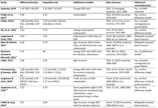
Table 1. Cross-national, inter-temporal STIRPAT studies estimating the drivers of CO2 emissions. Values indicate elasticities of emissions with

respect to changes in GDP per capita (income) and population size.

Study Affluence/income Population size Additional variables Data structure Addressed nonstationarity? Sadorsky, 2014 1.14 (SR); 0.90 (LR) 1.33 (SR); 2.52 (LR) Energy-GDP ratio TSCS: 16 emerging

countries, 1971-2009

Yes, via AMG estimator

Knight et al., 2013 a

0.59 2.25 Urbanization TSCS: 29 OECD countries,

1970-2007

Yes, via first difference model

Liddle, 2013c c 1.00 (overall); 0.44 (HI); 1.00 (MI); 0.97 (LI)

1.05 (overall); 0.68 (HI); 0.86 (MI); 0.70 (LI)

TSCS: 23 HI, 25 MI, & 37 LI countries, 1971-2007

Yes, via panel cointegration & panel FMOLS

Zhu et al., 2012 1.12 0.79 Energy consumption; urbanization

TSCS: 20 non-OECD countries, 1992-2008

Yes, via first difference model

Jorgenson & Clark, 2012

0.93 1.55 Urbanization; trade share of

GDP

Panel: 86 countries, 1960-2005 at 5-yr intervals

Mitigated via panel data structure

Menz & Welsch, 2012 a

0.36 0.78 Age structure; birth cohort;

share of electricity from coal; urbanization

Panel: 26 OECD countries; 1960-2005 at 5-yr intervals

Mitigated via panel data structure

Martinez-Zarzoso & Maruotti, 2011 a

0.72 NS Energy-GDP ratio; GDP share

for industry; urbanization

TSCS: 88 non-OECD countries, 1975-2003

Yes, via difference

model b

Liddle, 2011 c 1.06 2.35 Age structure TSCS: 22 OECD countries, 1960-2007

Yes, via panel cointegration & panel FMOLS

Poumanyvong & Kaneko, 2010 a

1.08 (overall); 0.83 (HI); 0.99 (MI); 2.50 (LI)

1.12 (overall); 1.12 (HI); 1.23 (MI); 1.75 (LI)

Energy-GDP ratio; GDP share for service & industry; urbanization

TSCS: 33 HI, 43 MI, and 23 LI countries, 1975-2005

Yes, via first difference model

Jorgenson & Clark, 2010 a

0.65 (overall); 0.95 (OECD); 0.64 (non-OECD)

1.43 (overall); 1.65 (OECD); 1.27 (non-OECD)

Trade as share of GDP; urbanization

Panel: 22 DC and 64 LDC; 1960-2005 at 5-yr intervals

Yes, via first difference model & panel structure

Jorgenson et al., 2010 a e

0.33 0.70 Share population aged 15-64;

GDP share for manufacturing; urbanization; share

population living in urban slums

TSCS: 57 LDC, 1990-2005 Yes, via first

difference model

Liddle & Lung, 2010 a

0.57 0.69 Age structure; energy-GDP

ratio for industry; Share of

Panel: 17 OECD countries, 1960-2005 at 5-yr

primary energy from nonfossil fuels; urbanization

intervals

York, 2008 0.50 1.87 Aged dependency ratio; Urbanization; FDI as share of GDP; military personnel per 1000

TSCS: 15 FSR, 1992-2000 No

Martinez-Zarzoso et al., 2007 a

0.42 (overall); 0.15 (15 old EU); 0.34 (8 new EU)

NS (overall); 0.71d (15 old EU); 2.73 (8 new EU)

Energy-GDP ratio; GDP share for industry

TSCS: 23 EU countries, 1975-1999

Yes, via first difference model

York, 2007 e 0.70 2.75 Share of old dependent population; urbanization

TSCS: 14 EU countries; 1960-2000

No

Fan et al., 2006 f 0.30 (overall);0.54 (HI); 0.21 (UMI); 0.28 (LMI); 0.33 (LI)

0.68 (overall); 0.57 (HI); 0.33 (UMI); 0.44 (LMI); 0.26 (LI)

Share population aged 15-64; Energy-GDP ratio;

urbanization

TSCS: 218 countries, 1975-2000

No

Cole &

Neumayer, 2004 a

0.89 0.98 Age structure; Average

household size; Energy-GDP ratio; GDP share for

manufacturing; urbanization

TSCS: 86 countries, 1975-1998

Yes, via first difference model

Shi, 2003 0.80 0.83 (HI); 1.42 (UMI); 1.97 (LMI); 1.58 (LI)

GDP share for manufacturing & service

TSCS: 88 countries, 1975-1996

No

Notes: a estimations were performed in first differences or with a lagged dependent variable; and thus, those elasticities could be interpreted as short-run (as

opposed to long-run). b Martinez-Zarzoso & Maruotti perform panel unit root tests that suggest the variables are panel I(0); however, as discussed in the text,

this is a highly unusual result; and thus, we report their results from a difference generalized method of moments model. c dependent variable was CO2

emissions from all (domestic) transport activity. d statistically significant at p < 0.10. e dependent variable was total energy use. f

estimations performed via partial least squares; hence results may not be compatible with other studies.

TSCS: time-series cross-section. NS= not statistically significant at the p < 0.10 level or higher. SR=short run. LR=long run. AMG=augmented mean group. FMOLS=fully

modified ordinary least squares. OECD=Organization for Economic Cooperation and Development; EU=European Union; FSR=former Soviet republics; DC=developed

Table 2. Summary statistics and correlations (all variables in natural logs).

Variable Obs Mean Std. dev. Min. Max.

CO2 3280 3.37 2.05 -1.66 8.98

A 3280 8.64 1.27 5.48 11.21

Pop 3280 16.67 1.49 12.25 21.02

IEI 3144 -2.21 0.83 -6.55 0.49

Sh nff 3277 -3.47 1.65 -9.24 -0.18

Correlations CO2 A Pop IEI Sh nff

CO2 1

A 0.519 1

Pop 0.648 -0.235 1

IEI 0.157 -0.176 0.100 1

Sh nff 0.112 0.340 -0.072 -0.022 1

Table 3. Cross-sectional dependence: Absolute value mean correlation coefficients and Pesaran (2004) CD test.

Variables

Panels Log CO2 Log A Log Pop Log IEI Log Sh n ff

OECD countries 0.70 0.96 0.90 0.72 0.57

(26) (18.3*) (108.1*) (87.9*) (51.5*) (33.0*)

Non-OECD countries (54)

0.76 (134.5*)

0.65 (93.1*)

0.98 (209.3*)

0.43 (17.2*)

0.50 (29.0*)

Notes: CO2 is aggregate carbon emissions; A is real GDP per capita; Pop is population; IEI is

Table 4. Heterogeneous panel STIRPAT estimations. Aggregate carbon emissions dependent variable. 95% confidence intervals in brackets.

All countries (80) OECD countries (26) Non-OECD countries (54)

CMG AMG CMG AMG CMG AMG

Log A 0.81** [0.69 0.93] 0.87** [0.74 0.99] 0.58** [0.41 0.75] 0.71** [0.58 0.84] 0.89** [0.74 1.04] 0.83** [0.71 0.95]

Log Pop 1.38* [0.98 1.78] 1.85** [1.29 2.41] 0.81* [0.03 1.59] 1.26** [0.33 2.20] 1.32** [0.95 1.70] 1.87** [1.61 2.15]

Log IEI 0.18** [0.15 0.22] 0.18** [0.14 0.23] 0.17** [0.10 0.24] 0.16** [0.09 0.24] 0.17** [0.12 0.21] 0.19** [0.13 0.25]

Log sh nff -0.14** [-0.17 -0.10] -0.13** [-0.17 -0.10] -0.12** [-0.16 -0.07] -0.13** [-0.17 -0.08] -0.13** [-0.17 -0.09] -0.13** [-0.18 -0.09]

Obs 3141 3141 1045 1045 2096 2096

RMSE 0.054 0.064 0.030 0.036 0.063 0.081

Order of integration

I(0) I(0) I(0) I(0) I(0) I(0)

Mean rho 0.17 0.17 0.14 0.16 0.18 0.18

CD (p) 2.3 (0.02) -0.5 (0.60) 0.2 (0.87) -1.2 (0.25) 0.3 (0.76) 0.9 (0.36)

Notes: A is real GDP per capita; Pop is population; IEI is industry energy intensity; sh nff is share of nonfossil fuels in primary energy. Obs is observations, and RMSE is the root mean squared error. * and ** indicate statistical significance at the 5% and 1% levels, respectively.

Table 5. Heterogeneous panel estimations. Carbon emissions per capita dependent variable. 95% confidence intervals in brackets.

OECD countries (26) Non-OECD countries (54)

CMG AMG CMG AMG

Log A 0.57*

[0.37 0.77]

0.75* [0.61 0.89]

0.97* [0.79 1.14]

0.96* [0.83 1.09]

Log IEI 0.17*

[0.10 0.25]

0.16* [0.07 0.25]

0.20* [0.14 0.26]

0.20* [0.12 0.28]

Log sh nff -0.12* [-0.16 -0.08]

-0.13* [-0.18 -0.09]

-0.13* [-0.16 -0.09]

-0.12* [-0.17 -0.07]

Obs 1045 1045 2096 2096

RMSE 0.034 0.039 0.071 0.092

Order of integration I(0) I(0) I(0) I(0)

Mean rho 0.18 0.19 0.19 0.19

CD (p) -0.1 (0.94) -1.3 (0.20) 1.4 (0.15) 0.9 (0.35)

Notes: A is real GDP per capita; IEI is industry energy intensity; sh nff is share of nonfossil fuels in primary energy. Obs is observations, and RMSE is the root mean squared error. * indicates statistical significance at the 0.1% level.

Figure 1. Individual country population elasticity estimates (from AMG) and the country average GDP per capita for the sample period (for all countries). Trend line and R-squared also shown.

R² = 0.0054

-4 -2 0 2 4 6 8 10 12

$- $5,000 $10,000 $15,000 $20,000 $25,000 $30,000 $35,000 $40,000 $45,000

Population elasticity

Figure 2. Individual country population elasticity estimates (from AMG) and the natural log of country average population for the sample period (for all countries). Trend line and R-squared also shown.

R² = 0.0092

-4 -2 0 2 4 6 8 10 12

12 13 14 15 16 17 18 19 20 21 22

Population elasticity

Figure 3. Individual country income elasticity estimates (from AMG) and the country average GDP per capita for the sample period (for all countries). Carbon emissions per capita is the dependent variable. Trend line, equation, and R-squared also shown.

y = 2E-10x2_{- 4E-05x + 1.2649}

R² = 0.335

-1 -0.5 0 0.5 1 1.5 2 2.5 3 3.5

$- $5,000 $10,000 $15,000 $20,000 $25,000 $30,000 $35,000 $40,000 $45,000

Income elasticity

Appendix A. List of countries (by World Bank three letter code).

OECD (26) Non-OECD (54)

AUS IRL AGO EGY NPL

AUT ISL ALB ETH PAK

BEL ITA ARG GAB PAN

CAN JPN BGD GHA PER

CHE KOR BGR GTM PHL

DEU LUX BOL HND SDN

DNK NLD BRA IDN SLV

ESP NOR CHL IND TGO

FIN NZL CHN IRN THA

FRA POL CIV JAM TUN

GBR PRT CMR KEN TUR

GRC SWE COG LKA URY

HUN USA COL MAR VEN

CRI MEX VNM

CUB MMR ZAF

DOM MOZ ZAR

DZA MYS ZMB

Appendix B. Unit root tests

Appendix Table B.1 displays the results of the Pesaran (2007) panel unit root test (CIPS).

The null hypothesis of the test is nonstationarity; thus, if the null is rejected in levels, the series is

assumed to be I(0); however, if the null fails to reject when in levels, but is rejected when in first

differences, the series is assumed to be I(1). The CIPS test results suggest that carbon emissions,

affluence/income, and industrial energy intensity are I(1); however, the results for population are

ambiguous—depending on the choice of lag structure and trend inclusion, it could be I(0) or I(1).

Appendix Table B.1

Yet, population is a classic stock variable: population in period t is exactly equal to the

population in period t-1 less the deaths, plus the births and net migration (that occurred over the

intervening time). In other words, unlike for GDP, we do understand the “data generation

process” for population, and that process is the same everywhere. Unless the change in

population (births and net migration less deaths) is equal to zero over time, population likely

does not have a constant mean (i.e., is not stationary). Innovations to fertility and mortality rates

(e.g., education of girls leading to changes in desired family size or wide-spread adoption of

health/safety measures like hand-washing) do cause permanent changes; but after an adjustment

period, we would expect fertility and mortality rates to be constant. Therefore, we expect

population to be a I(1) variable, i.e., trending over time, but its change or first difference has a

(nonzero) constant mean.

The problem in calculating population’s order of integration (as demonstrated by the

results in Appendix Table B.1) is likely a manifestation of the poor/limited power of unit root

tests when the time dimension is relatively short. (Time-series econometricians consider 50

countries via data compiled by Angus Madison

(http://www.ggdc.net/MADDISON/oriindex.htm). Now the CIPS test produces a highly robust

result of I(1). Appendix Table B.2 shows that with lags varying from zero to eight and with or

without a trend in the regression, population is confirmed as a I(1) variable at the highest levels

of significance.

Appendix Table B.2

Appendix Table B.1. Pesaran (2007) panel unit root tests for 80 country sample.

Variables in Levels

Constant w/o trend Constant w/ trend

No. lags 1 2 3 1 2 3

Log Pop 0.000 0.995 0.996 0.000 0.001 0.001

Log CO2 0.042 0.150 0.353 0.998 0.999 1.000

Log A 0.998 1.000 0.998 0.653 0.993 0.828

Log IEI 0.068 0.896 0.778 0.620 0.999 0.999

Log sh nff 0.000 0.000 0.070 0.000 0.000 0.033

Variables in first differences

No. lags 1 2 3 1 2 3

Log Pop 0.000 0.000 0.000 0.000 0.000 0.000

Log CO2 0.000 0.000 0.000 0.000 0.000 0.000

Log A 0.000 0.000 0.000 0.000 0.000 0.000

Log IEI 0.000 0.000 0.000 0.000 0.000 0.000

Log sh nff 0.000 0.000 0.000 0.000 0.000 0.000

Notes: P-values shown for null hypothesis of I(1). Pop is population. CO2 is aggregate carbon

Appendix Table B.2. Pesaran (2007) panel unit root tests for population of a panel of 19 OECD countries, 1820-2008.

Constant w/o trend Constant w/ trend Number of

lags

level First difference

conclusion level First difference

conclusion

0 3.12

(1.00)

-15.55 (0.00)

I(1) 11.04 (1.00)

-15.80 (0.00)

I(1)

1 1.44

(0.92)

-13.76 (0.00)

I(1) 6.15

(1.00)

-13.86 (0.00)

I(1)

2 1.86

(0.96)

-10.76 (0.00)

I(1) 5.75

(1.00)

-10.32 (0.00)

I(1)

3 1.52

(0.94)

-9.76 (0.00)

I(1) 5.35

(1.00)

-9.19 (0.00)

I(1)

4 1.91

(0.97)

-7.72 (0.00)

I(1) 5.68

(1.00)

-7.00 (0.00)

I(1)

5 1.58

(0.94)

-6.64 (0.00)

I(1) 5.11

(1.00)

-5.66 (0.00)

I(1)

6 1.51

(0.94)

-5.16 (0.00)

I(1) 5.19

(1.00)

-3.93 (0.00)

I(1)

7 1.16

(0.88)

-4.62 (0.00)

I(1) 4.89

(1.00)

-3.42 (0.00)

I(1)

8 1.10

(0.86)

-3.71 (0.00)

I(1) 4.91

(1.00)

-2.44 (0.01)

I(1)

Notes: Pesaran (2007) Z-statistic with associated p-value (in parentheses) shown. Null hypothesis is the series is I(1).

Countries: Australia, Austria, Belgium, Denmark, Finland, France, Germany, Greece, Ireland, Italy, Japan, Netherlands, Norway, Portugal, Spain, Sweden, Switzerland, United Kingdom, and United States.

Appendix C: Additional time series, cross section estimators

POLS: Pooled OLS with time dummies

2FE: Fixed effects with time dummies (two-way fixed effects)

2FE-LDV: Fixed effects with lagged dependent variable and time dummies

FE-Prais: Prais-Winsten serial correlation correction with country and time dummies

FD-OLS: OLS with variables in first differences and time dummies

P-FMOLS: Pooled version of Fully Modified OLS. FMOLS involves a semi-parametric correction for serial correlation and endogeneity.

P-DOLS: Pooled version of Dynamic OLS. DOLS involves adding leads and lags of the first differences of the explanatory variables in order to address

endogeneity and serial correlation. One lead and one lag of each are added.

MG-FMOLS: Mean group FMOLS, where the panel estimates are the average over the individual cross-section FMOLS estimates.

MG-DOLS: Mean group DOLS, where the panel estimates are the average over the individual cross-section DOLS estimates. One lead and one lag of each RHS variable and common time dummies were added. Performed by STATA command xtpedroni, which was developed by Timothy Neal.

Appendix Table C.1. Additional STRIPAT estimations on 80 country sample. Aggregate carbon emissions dependent variable.

Pooled Estimators Heterogeneous Estimators POLS 2FE 2FE-LDV FE-Prais FD-OLS P-FMOLS P-DOLS MG-FMOLS MG-DOLS Log A 1.25** 1.14** 0.18** 1.01** 0.80** 0.91** 0.79** 0.84** 1.09**

Log Pop 1.11** 1.87** 0.29** 1.10** 1.73** 1.23** 1.14** 1.11** 1.91**

Log IEI 0.51** 0.31** 0.044** 0.27** 0.24** 0.32** 0.20** 0.21** 0.20**

Log sh nff -0.11** -0.07** -0.02** -0.07** -0.07** -0.10** -0.08** -0.17** -0.21**

LDV/AR 0.86** 0.98

Obs 3141 3141 3075 3141 3061 3061 2901 3061 2901

Order of integration

I(1) I(1) I(0) I(1) I(0) I(1) I(0) I(1) I(0)

Mean rho 0.54 0.45 0.16 0.54 0.14 0.51 0.21 0.51 0.15

CD (p) -3.7 (0.00) -2.5 (0.01) -2.3 (0.02) -3.6 (0.00) -2.2 (0.03) 6.5 (0.00) 5.3 (0.00) 4.2 (0.00) 1.8 (0.07)

Notes: A is real GDP per capita; Pop is population; IEI is industry energy intensity; sh nff is share of nonfossil fuels in primary energy. LDV/AR refers to the coefficient for the lagged dependent variable or AR term. Obs is observations. ** indicates statistical significance at the 1% level.

Diagnostics: Order of integration of the residuals is determined from the Pesaran (2007) CIPS test: I(0)—stationary, I(1)—

nonstationary. Mean rho is the mean absolute correlation coefficient of the residuals from the Pesaran (2004) CD test. CD is the test statistic from that test along with the corresponding p-value in parentheses. The null hypothesis is cross-sectional independence.

Appendix D. Time span robustness of long-run affluence and population estimations. Aggregate carbon emissions dependent variable. Panel coefficients for population and affluence along with their 95% confidence intervals in brackets shown.

Non-OECD countries (45) OECD countries (25)

Time CMG AMG CMG AMG

span Log A Log Pop Log A Log Pop Log A Log Pop Log A Log Pop

1971-1991 0.88 [0.68 1.07] 0.82 [020 1.44] 0.89 [0.72 1.06] 0.93 [0.64 1.22] 0.68 [0.41 0.93] 0.97 [-0.24 2.18] 0.78 [0.63 0.92] 0.95 [-0.35 2.25] 1975-1995 0.66 [0.47 0.85] 3.13 [0.002 6.26] 0.82 [0.62 1.01] 1.03 [0.70 1.36] 0.55 [0.34 0.76] 0.26 [-0.99 1.50] 0.73 [0.59 0.88] 1.26 [-0.08 2.59] 1980-2000 0.74 [0.61 0.88] -1.07 [-4.40 2.27] 0.72 [0.50 0.94] 1.26 [0.58 1.05] 0.41 [0.13 0.69] 0.21 [-1.72 2.15] 0.66 [0.48 0.83] 1.22 [0.27 2.18] 1990-2011 0.86 [0.64 1.07] 0.80 [-0.53 2.13] 0.82 [0.58 1.05] 1.65 [1.35 1.95] 0.52 [0.24 0.81] 0.28 [-0.32 0.89] 0.64 [0.50 0.78] 1.00 [0.09 1.90] 1985-2005 0.92 [0.72 1.13] 0.07 [-1.40 1.53] 0.77 [0.60 0.94] 1.03 [0.58 1.48] 0.50 [0.18 0.82] -0.36 [-2.66 1.94] 0.63 [0.44 0.83] 0.48 [-0.23 1.19] 1971-1996 0.82 [0.64 1.00] 0.78 [0.03 1.53] 0.90 [0.71 1.09] 0.99 [0.64 1.33] 0.72 [0.53 0.91] 0.92 [-0.005 1.85] 0.72 [0.58 0.85] 1.01 [0.15 1.86] 1975-2000 0.78 [0.60 0.97] 1.55 [-0.39 3.48] 0.88 [0.66 1.09] 1.21 [0.88 1.54] 0.51 [0.31 0.70] 0.53 [-0.46 1.54] 0.65 [0.51 0.78] 1.63 [0.34 2.92] 1980-2005 0.85 [0.68 1.02] -0.002 [-1.94 1.93] 0.91 [0.72 1.11] 1.27 [0.96 1.59] 0.44 0.20 0.67] -0.08 [-1.68 1.52] 0.64 [0.46 1.35] 0.69 [0.02 1.35] 1985-2011 1.04 [0.81 1.27] 0.56 [-0.74 1.86] 0.81 [0.64 0.98] 1.34 [1.07 1.64] 0.55 [0.27 0.84] 0.01 [-0.74 0.76] 0.65 [0.51 0.79] 0.62 [0.003 1.24] 1971-2001 0.82 [0.64 1.00] 0.86 [0.15 1.58] 0.96 [0.78 1.14] 1.13 [0.80 1.45] 0.66 [0.45 0.87] 0.77 [-0.19 1.74] 0.67 [0.52 0.80] 1.21 [0.12 2.30] 1975-2005 0.90 [0.75 1.06] 1.03 [-0.53 2.59] 0.97 [0.81 1.13] 1.20 [0.92 1.48] 0.51 [0.30 0.72] 0.76 [-0.41 1.92] 0.68 [0.53 0.83] 1.10 [0.23 1.97] 1980-2011 0.90 [0.73 1.08] 0.70 [-0.59 1.99] 0.87 [0.69 1.04] 1.38 [1.12 1.64] 0.51 [0.31 0.72] 0.58 [-0.23 1.40] 0.62 [0.46 0.78] 0.91 [0.53 1.29]