A ranking of VAR and structural models in forecasting

Munich Personal RePEc Archive

A ranking of VAR and structural models

in forecasting

Bentour, El Mostafa

Arab Planning Institute, Kuwait

15 January 2015

Online at

https://mpra.ub.uni-muenchen.de/61502/

A ranking of VAR and structural models in forecasting

EL Mostafa Bentour*,

Arab Planning Institute, Shuwaikh Educational, Kuwait.

Abstract

This paper ranks economic forecasts performances for two structural models against a

benchmark of time series models, VAR and ARIMA, according to a set of statistical measures

calculated for the main economic aggregates. The period of analysis covers twenty years for

annual data (1985-2004) and 28 quarters for quarterly models (1998:1-2004:4). Furthermore,

models are tested to see whether predictions contain additional information more than the one

showed by a random walk process (Fair-Shiller, 1987). Results show a net supremacy of VAR

models over structural models and have significant contribution to information than the one

contained in the random walk process.

JEL Classification: C180, C320, C530.

Keywords: Random Walk, Structural models, Theil Criterion, VAR models.

1. Introduction

To achieve economic forecasts, practitioners use a variety of methods. Some prefer to use an

implicit scheme they are built from the knowledge of the economy; the expert judgment. Others

prefer using the formal diagram based on the economic theory; the structural macroeconomic

models. The third category uses statistical models; time series models instead of structural

models. The mix of two or more of these methods is generally used to enhance the quality of

forecasts (consensus forecast). Despite their ultimate usefulness, models are subject to critics. For

some economists, structural macroeconomic models are making room too much to theoretical

expectations and prefer to use time series models, especially Vector Auto Regressive (VAR)

models in which the place of these expectations is limited. Furthermore, VAR models appeared

in the early 80s as a questioning of the methodology underlying the construction and the use of

structural models (Sims, 1980) and following the famous Lucas’s critic to structural models.

In practice, the advantages of a type over the other depend on the constraints related to the

availability of information as well as the ability to capture agents’ economic behaviors. The

advantage of VAR models, for example, is that their estimate is flexible and less demanding in

information and time. In addition, these models allow easily integrating new data. But the VAR

models have also their drawbacks: The most one is that standard VAR models are assimilated to

"black boxes" because they lack description and economic explanation of the linkages between

variables as they do not refer to any economic theory framework. These weaknesses make such

models an additional tool of forecasting and cannot totally substitute the structural models.

Structural models require the development of an economic theory and an accounting

framework. This allows explaining linkages between variables thus providing forecasts

their designs and updates.

Despite the weaknesses that could surround all these type of models, they remain vital in

economic decision, especially in a changing world relying on systems increasingly complicated.

Therefore, economic forecasting, despite induced errors, remains essential to policymakers.

The Department of Studies and Financial Forecasts (DSFF)1, assigned as missions to advise

the Government in terms of economic policy and business cycle analysis has developed a set of

tools and models for this purpose. The department constructed two relatively large size structural

models that aim to provide an image of the actual functioning of the economy. The first one is on

quarterly frequency data and the other one is on annual frequency data. These models are used in

forecasting and impact assessment of Government policies and foreign shocks.

To assess the accuracy of the two models in forecasting, we constructed a set of time series

models; autoregressive integrated moving average (ARIMA) and vector autoregressive (VAR)

models, to evaluate the performances of structural models against this benchmark of statistical

models. The assessment is made based on comparison of the generated forecasting errors. This

comparison is undertaken based on a set of statistical criteria and the content of information

method (Fair and Shiller, 1987).

The next section presents a brief presentation of the compared models. The third section

describes the methodology of comparison. The fourth part summarizes the results and the fifth

one concludes.

2. An overview of the compared models

Two macroeconomic structural models were developed at the Department of Studies and

Financial Forecasts to ensure the role of macroeconomic forecasts and assessment of economic

policies. This section briefs these structural models as well as the constructed competing ARIMA

and VAR models. These models use time series data from the structural models databases. The

databases are constructed for the needs of the two structural models using different national

sources from which the National Accounts data provided by the High Commissioning of

Planning (www.hcp.ma) is the main source.

2.1. The macroeconomic structural models

The first model is a structural quarterly macroeconomic model abbreviated by SQMM. Over

the period 1998-2002, the DSFF assigned to the "Conference Board of Canada" the construction

of this model for the Moroccan economy. The objective of this model is to meet the needs of the

Department in terms of forecasting, understanding of macroeconomic developments and

assessment of economic policy measures and impact of external shocks. This model describes the

Moroccan economy through 375 equations, from which 187 equations reflect the behaviors of

economic agents. The number of control variables included in the model are of 86 including 20

variables related to the fiscal policy and 10 to the financial and monetary policies. The rest are

exogenous variables regarding the international environment or demographics. The choice of

specifications adopted was often imposed by arguments from theoretical or empirical

considerations. The main difficulty in this model refers to deficiencies related to the information

system on the quarterly data. The large number of constructed quarterly time series weakens the

performance of this model.

The second structural model is an annual macroeconomic model named hereafter SAMM.

The establishment of this model was conducted with the collaboration of “EUROSTAT Bureau”,

Union. The goal is to replace the old annual model used previously for the preparation of the

macroeconomic framework underlying the Finance Act. The old one was actually a simple sheet

in Excel developed in 1996 and is not taken into account by the current comparison. The

principal missions of the SAMM are: to deliver simulated scenarios of economic policies, to

study the effects of exogenous shocks and to display forecasts in the short and medium term.

The general theoretical framework of the two structural models is based on a New Keynesian

structure. Some patterns have been slightly modified to take into account the characteristics of

the Moroccan economy, and to better reproduce the main economic linkages of the country. For

this, appropriate treatments were granted to any phenomenon that presents a particular aspect for

the country and contributes by a significant weight in the economy. This concerns first of all the

agricultural sector which is treated as a supply side determined mainly by the frequency of the

weather conditions.

2.2 ARIMA and VAR models:

The two structural models of the DSFF are compared to a set of ARIMA and VAR models

constructed for a number of key aggregates namely; GDP, Consumption, Gross Fixed Capital

Formation, Export and Import for the annual data. For the quarterly data, GDP and added values2

by sector are considered.

ARIMA model stands for Autoregressive Integrated Moving Average. It is defined as a

stationary process function of its own lags (the AR component), and a moving average of

stochastic errors (the MA component). The implementation of ARIMA models are done

2

following the Box-Jenkins methodology. This method follows a number of steps. The first step is

to transform data to stabilize the series and determine the order of integration d by appropriate

stationary tests (Augmented Dickey-Fuller and Phillips-Peron tests). The second step is to

determine the number of lags p for the autoregressive component by studying the autocorrelation

function (ACF) and the order q for the Moving Average component MA (q) by considering the

partial autocorrelation functions (PACF). The third step is to estimate the candidate models and

run information criteria to select the best one. The fourth step run tests for autocorrelations and

white noise residuals. In case of failure in the fourth step, procedure is repeated from the second

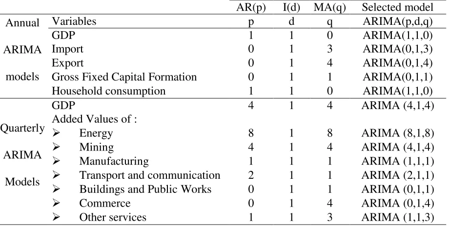
step, otherwise the model is ready to use for forecast. Table 1 summarizes the best candidate

models for constructed annual and quarterly ARIMA. All the models have in common an

integrated component of first order; all the series are non stationary.

Table 1: ARIMA models

AR(p) I(d) MA(q) Selected model Annual

ARIMA

models

Variables p d q ARIMA(p,d,q) GDP 1 1 0 ARIMA(1,1,0) Import 0 1 3 ARIMA(0,1,3) Export 0 1 4 ARIMA(0,1,4) Gross Fixed Capital Formation 0 1 1 ARIMA(0,1,1) Household consumption 1 1 0 ARIMA(1,1,0)

Quarterly

ARIMA

Models

GDP 4 1 4 ARIMA (4,1,4) Added Values of :

 Energy 8 1 8 ARIMA (8,1,8)

 Mining 4 1 4 ARIMA (4,1,4)

 Manufacturing 1 1 1 ARIMA (1,1,1)

 Transport and communication 2 1 1 ARIMA (2,1,1)

 Buildings and Public Works 0 1 1 ARIMA (0,1,1)

 Commerce 0 1 4 ARIMA (0,1,4)

 Other services 1 1 3 ARIMA (1,1,3)

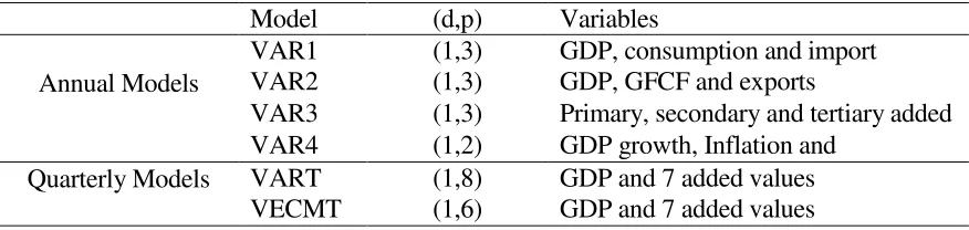
On the contrary of univariate time series ARIMA, VAR models are a vector of two or more

the past values of the other components of the vector to a finite order p (lags). The important step

in VAR modeling is the determination of the order of such lags.

All series in the previous section and others involved in the VAR models are revealed to be

integrated of order 1, i.e. non-stationary and are made stationary by differentiation. Therefore, all

variables are introduced in first differences. Lags, orders of VAR models p, are determined by

the Akaike and Schwartz information criteria. We develop a range of models presented in table 2,

namely VAR1, VAR2, VAR3 and VAR4 for annual data, VART for eight quarterly variables

and VECMT is the same model in error correction form.

Table 2: VAR models

Model (d,p) Variables

Annual Models

VAR1 (1,3) GDP, consumption and import VAR2 (1,3) GDP, GFCF and exports

VAR3 (1,3) Primary, secondary and tertiary added VAR4 (1,2) GDP growth, Inflation and

Quarterly Models VART (1,8) GDP and 7 added values VECMT (1,6) GDP and 7 added values

3. Methodology

The quality of a prediction method with respect to another is measured by a set of statistical

criteria. The approach is to rank the models over a period of time according to the rule that the

best model is the one on which such criteria are minimized. However, other economic criteria

may provide a comparison, especially based on the content of information of the forecast. The

economic criteria are indeed necessary especially when two forecasted values are inseparable in

terms of statistical criteria. Other measures could be the ability to forecast structural changes or

turning points. However, (Jorgenson et al. 1970) conclude that the models that fit best are those

The forecast error is defined as the difference between the expected value Yˆ_jt and the

observed valueY_jt . The statistical measures used for comparison are all based on the average of

forecast errors committed in a given period1N. The comparison can be performed on the whole

common history for all models as it may be limited to a given period or some economic cycles.

3.1. Statistical measures

The first and simplest measure is the mean error (ME). It describes the average of forecast

errors over a given period. For example, a negative average error for the percent change in real

GDP reveals that this variable was underestimated during the forecast period. This measure is

however useless as negative values can be canceled by positive ones. It is formulated as:

N Y Y ME N t t jt



The second measure is the mean absolute error (MAE) defined as the average of the absolute

values of forecast errors. It handles the ME disadvantage and is formulated as:

N Y Y MAE N t t jt



The third measure is the square root of the mean squared errors (SRMSE). This measure

is similar to the previous one except that this time, the penalty associated with the forecast error

increases squarely and significant errors are penalized more than smaller ones. This measure is

N Y Y SRMSE

N

t

t jt



 

 1

2

)

ˆ

(

(3)

The coefficient of Theil U is the fourth proposed measure. In fact, SRMSE can be inefficient;

this is particularly the case when the measuring unit of the data is different or when we compare

levels. Indeed, an error arising from a forecast expressed in thousands of currency unit may not

have the same value as a result of an error expressed in millions of the same currency. To remedy

to this inconvenience, the naive model is used to construct the relative error for each variable and

each forecast model. To measure the relative contribution, Theil proposed a ratio, called U, of

SRMSE of the compared model mto that one provided by the naive modelnm. The naïve model

forecasts the next period as the outcome of the current year. In case of U 1, it indicates that the

studied model performs as the naïve model, U 1, the studied model is better than the naïve

model and U 1 is the opposite. The ratio is:

nm m

SRMSE SRMSE

U  (4)

Another way to calculate the Theil coefficient is to standardize SRMSE using the standard

deviation of changes in the variable provided during a historical period (1985- 2004). Using the

standard deviation of changes in the economic variable, we normalize the forecast error and can

thus compare the performance of prediction models for all variables provided not only for a

variable taken individually. This method is preferable to univariate analysis. We name this

N Y Y SRMSE SRMSSE N t t m



3.2. Fair and Shiller procedure

It is difficult to say that the best forecast or the best model compared to others is the one who

has the best statistical criterion. If this is the case, it is to assume consistency between forecast

accuracy and optimality of the use that is actually in a decision making framework: the

opportunity to invest as example.

However, the criterion of information content proposed by (Fair and Shiller, 1987) enhances

the previous methods of selecting the best forecasts. This method asserts that prediction is better

than another when it contains more information than the other compared to a simple random

walk model. Another advantage is that even when a first model is considered better than another

on the basis of a statistical test, it is possible that the second contains additional information other

the one contained in a random walk process compared to the first model.

Fair and Shiller construct a hypothesis test based on the following regression:

t tk tk

tk ze ze

ze  . 1 . 2  (6)

Where ; ze_tk is the percent change of the observed variable zbetween tand tk. For

1



k , it is only the instantaneous growth rate. 1

tk

ze and 2

tk

ze are respectively the errors of forecasts

issued from the first and the second model for the variablezbetween t and tk. The null

hypothesis associated test is that both models provide no additional information at the level of the

0 = and 0 = : )

(H₀   (7)

The alternative hypothesis test is at least one of the two coefficients is non null:

0 and/or 0

: )

(H₁     (8)

If β (respectively γ) is significantly non null, then the forecast from model 1 (respectively

from model 2) contains additional information absent in the prediction provided by the model of

random walk and there is no additional information from prediction provided by model 2

(respectively model 1). When both coefficients are significantly different from zero at the same

time, there is significant economic information in the two forecasts from the two models other

than the information provided by the random walk model.

4.Comparative Analysis

The comparison presented in this section was conducted over the period 1985 to 2004 for

annual forecasts. The annual comparison was made considering a sample of five economic

aggregates: gross domestic product (GDP), consumption (C), gross fixed capital formation

(GFCF), imports of goods and services (MGS) and exports of Goods and services (XGS). As for

the analysis for the quarterly models, the comparison was made between 1998 and 2004 over a

sample of eight variables namely; GDP and added values of energy, mining, manufacturing,

construction and public works, commerce, transport and communication and other services. In

addition, the statistical measures are calculated for the variables growth rates instead of their

levels.

Forecasts by their ability to predict the future. This depends on the capacity to generate the

history. Assuming that a good model in forecasting is the one able to well simulate its data

history, the forecasted variables are drawn from backward simulations of the observed data. The

prediction error eMt at time tfor a model Mand a variable Yis defined as the difference

between the simulated Yˆ_Mt value and the observed valueYt: eMt  Yˆit  Yt

First, we evaluate models according to the annual statistical criteria, based on a single

variable (real economic growth). Second, we compare the models for a sample of variables (GDP

and its components) for each criterion separately. Finally, the same approach is used for the

quarterly comparison.

4.1.1 Ranking of annual models

Table 3 shows the statistical measures of forecast errors calculated for the annual real GDP

growth for the benchmark of the annual models. The last two columns of the table stand for ranks

of models according to the criterion of Theil U (Rank1) and SMRSSE (Rank2). It also includes

the average of measures over all models. Finally, measured criteria obtained from the naive

model are also considered for comparison in the last row.

Table 3: Rank of annual models based on the forecast of real GDP growth.

ME MAE SMRSE U SMRSS Rank1 Rank2 SAMM -0.65 2.13 2.67 0.29 0.28 5 4 ARIMA 0.47 4.61 5.86 0.64 0.97 6 6 VAR1 -0.10 0.85 1.04 0.11 0.11 1 1 VAR2 -0.36 1.01 1.30 0.14 0.14 3 3 VAR3 -0.18 0.92 1.26 0.14 0.13 2 2 Average -0.16 1.90 2.43 0.26 0.33 4 5 Naïve 0,00 7,32 9,16 1,00 0,97 7 7

This table shows that the three VAR models rank highest according to all measures, followed

by the annual model. These models are better than the average of the six models. The ARIMA

criteria, applied to a single variable, the real GDP growth, we conclude that the VAR models are

much better than the structural models in forecasting.

However, it is too early to make a judgment considering only one variable as a basis for

ranking. In what follows, we present a series of comparison on the basis of a sample of the main

economic variables according to statistical criteria. Table 4 shows calculated statistical measures

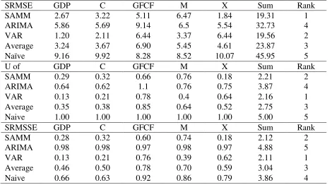
(SRMSE, U of Theil and SRMSSE) for the forecast errors from annual models (SAMM, ARIMA

and VAR) for a sample of variables (GDP, Consumption, Investment, Imports and Exports). We

also consider the average over the three annual models and the naïve model calculations in the

two last rows. The seventh column shows, for the models, the sum for each criterion over the five

variables. This allows ranking the models under this criterion for this sample of variables.

Table 4: Models’ Ranking based on statistical criteria

SRMSE GDP C GFCF M X Sum Rank SAMM 2.67 3.22 5.11 6.47 1.84 19.31 1 ARIMA 5.86 5.69 9.14 6.5 5.54 32.73 4 VAR 1.20 2.11 6.44 3.37 6.44 19.56 2 Average 3.24 3.67 6.90 5.45 4.61 23.87 3 Naïve 9.16 9.92 8.28 8.52 10.07 45.95 5 U of GDP C GFCF M X Sum Rank SAMM 0.29 0.32 0.66 0.76 0.18 2.21 2 ARIMA 0.64 0.62 1.1 0.76 0.75 3.87 4 VAR 0.13 0.21 0.78 0.4 0.64 2.16 1 Average 0.35 0.38 0.85 0.64 0.52 2.75 3 Naive 1.00 1.00 1.00 1.00 1.00 5.00 5 SRMSSE GDP C GFCF M X Sum Rank SAMM 0.28 0.32 0.60 0.74 0.18 2.12 2 ARIMA 0.98 0.98 0.97 0.98 0.97 4.88 5 VAR 0.13 0.21 0.76 0.39 0.62 2.11 1 Average 0.46 0.50 0.78 0.70 0.59 3.04 3 Naive 0.66 0.63 0.92 0.86 0.79 3.86 4

According to SRMSE measure, the annual model is nearly better than the VAR model while

model. The two models rank high over the single time series model (ARIMA) and the naïve

model. Over the five variables, the annual model is better in forecasting exports and investments

while the VAR is better in forecasting GDP, imports and consumption.

Based on annual data, we can say that the contribution of structural models in forecasting is

far from been superior to relatively simple methods of forecasting (VAR methods). Note also that

the VAR and the annual models are not clearly distinguishable as to the criterion of SRMSSE;

this measure is 2.12 for the annual model versus 2.11 for the VAR. This result suggests more

examination in terms of information contained in the forecast (Fair and Shiller procedure).

4.1.2 Ranking of quarterly models

Table 5 summarizes the results of statistical measures applied to the forecasts errors of real

GDP growth generated by the quarterly models. The last two columns of the table present a

ranking of the models according respectively to the Theil U (Rank1) and SRMSSE (Rank2)

measures.

Table 5: Ranking of quarterly models based on forecasts of real GDP growth

ME MAE SRMSE U Theil SRMSSE Rank1 Rank2 SQMM -0.26 1.97 2.75 1.77 2.10 5 5 VAR -0.04 0.64 0.73 0.35 0.56 1 1 ARIMA 0.01 1.49 1.86 1.20 1.42 4 4 Average -0.10 1.37 1.78 1.11 1.36 3 3 Naïve 1.28 1.39 1.55 1.00 1.18 2 2

The results confirm the improved performance of statistical models such as VAR models

with respect to structural models. Indeed, the VAR method ranks first according to all considered

criteria; U of Theil, SRMSSE, SRMSE and MAE. The quarterly model SQMM and ARIMA

perform less than the average and the naïve model.

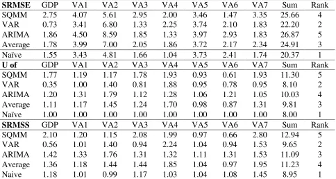
sectoral values added namely ; Energy (VA1), Mining (VA2), Manufacturing (VA3), Commerce

(VA4), Building and Public Works (VA5), Transport and Communication (VA6) and Other

Services (VA7). The last column of the table delivers the rank based on the sum of the measures

over the variables for each model.

Table 6: Ranking of quarterly models

SRMSE GDP VA1 VA2 VA3 VA4 VA5 VA6 VA7 Sum Rank SQMM 2.75 4.07 5.61 2.95 2.00 3.46 1.47 3.35 25.66 4 VAR 0.73 3.41 6.80 1.33 2.25 3.74 2.10 1.83 22.20 2 ARIMA 1.86 4.50 8.59 1.85 1.33 3.97 2.93 1.83 26.87 5 Average 1.78 3.99 7.00 2.05 1.86 3.72 2.17 2.34 24.91 3 Naïve 1.55 3.43 4.81 1.66 1.04 3.73 2.41 1.74 20.37 1

U of GDP VA1 VA2 VA3 VA4 VA5 VA6 VA7 Sum Rank SQMM 1.77 1.19 1.17 1.78 1.93 0.93 0.61 1.93 11.30 5 VAR 0.35 1.00 1.40 0.81 1.88 0.95 0.78 0.95 8.10 2 ARIMA 1.20 1.31 1.79 1.12 1.28 1.06 1.21 1.05 10.03 4 Average 1.11 1.17 1.45 1.24 1.70 0.98 0.87 1.31 9.81 3 Naïve 1.00 1.00 1.00 1.00 1.00 1.00 1.00 1.00 8.00 1

SRMSS GDP VA1 VA2 VA3 VA4 VA5 VA6 VA7 Sum Rank SQMM 2.10 1.20 1.15 2.08 1.99 0.97 0.66 2.80 12.94 5 VAR 0.56 1.01 1.40 0.94 2.24 1.04 0.94 1.53 9.65 2 ARIMA 1.42 1.33 1.76 1.31 1.32 1.11 1.31 1.53 11.09 3 Average 1.36 1.18 1.44 1.44 1.85 1.04 0.97 1.95 11.23 4 Naive 1.18 1.01 0.99 1.17 1.03 1.04 1.08 1.45 8.95 1

Over the three measures, the VAR model overcomes the structural quarterly model (SQMM).

Considering Theil measures (U and SRMSSE), the quarterly model is even surpassed by the

ARIMA model.

4.2. Comparison by Fair and Shiller procedure

According to the statistical criteria in the previous section, VAR models generally overcome

structural models. The following section applies the method of Fair and Shiller to rank the

models in terms of information contained in the forecasts. The same samples of variables used in

Table 7 shows the Failler and Shiller method applied to annual models for a sample of five

variables. The first row of the table tests the simultaneous nullity of two coefficients; the two

forecasts (of the VAR and the SAMM Models) do not provide any additional information other

than that contained in the random walk model. The second row tests the nullity of the coefficient

estimates of the VAR; the forecast of the VAR does not provide any additional information than

the one already contained in the random walk model, while the third row of the table tests the

same hypothesis for the forecast of the structural model SAMM. The last column of the table

shows the Fisher statistics read from the Fisher-Snedecor distribution table for a probability of

acceptance of the null hypothesis equal 5% and with 17 degrees of freedom (regression is made

on 20 observations, from 1985 to 2004, leading to 17 degrees of freedom after removal of 2

explanatory variables and the intercept). This statistic is compared to the empirical Fisher

statistics shown by the output of the regression for each variable. The number of tests is the

number of 15 linear regression models; two forecasts to test jointly and then separately for the

five variables in the sample.

Both VAR and annual models bring additional information than that already contained in the

forecast by a model of random walk for three variables: gross fixed capital formation, imports of

goods and services and exports of goods and services. By contrast, for GDP and consumption,

the null hypothesis of coefficients from simultaneous regression is accepted. Both models do not

provide any additional information other than that provided by forecasts of a random walk model

for the two variables; GDP and consumption. Individually, the tests confirm the superiority of

VAR models as to the contribution to information other than the one provided by the random

walk model. Indeed, except for the variable of imports of goods and services, where the annual

model outweighs the VAR, the null hypothesis is rejected for the VAR and the results are in

Table 7: Results of Fair and Shiller method applied to annual models

Annual GDP C GFCF M X F table at F(2,17) 1.02* 3.28* 6.20 5.12 6.28 3.59 F(1,17) 1.71* 6.01 12.74 3.17* 53.39 4.45 F(1,17) 0.39* 0.05* 0.05* 9.05 2.80*

*: significant at 5%, i.e. we accept the null hypothesis if : Ftable > Fempirical.

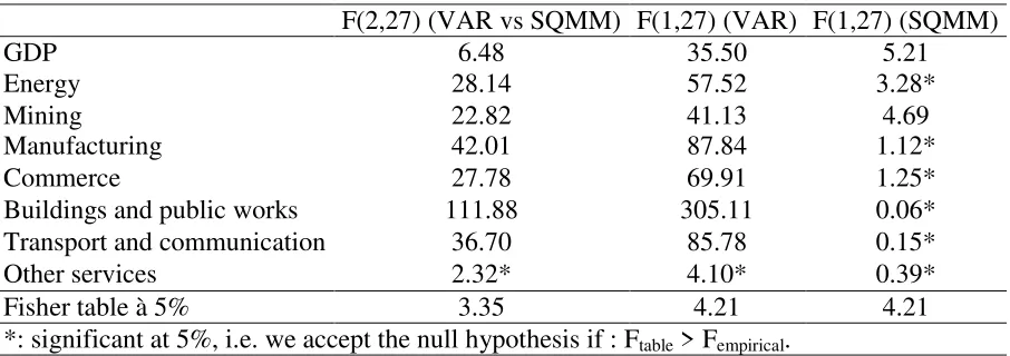
For quarterly models, results of Fair and Shiller regression are presented in table 8. The

first column presents the variables labels, the second shows the simultaneous regression Fisher

statistics for each variable while the two last columns show the Fisher p-values results for the

VAR and SQMM separately. The last row reports the Fisher table statistic at the 5% threshold.

Among the eight considered variables, only “other services” variable is generally not significant

at the simultaneous regression. For the rest of the variables, where the regression is significant,

the results are strong for the VAR model while the regression is significant only for two variables

for the quarterly model; GDP and Mining value added. This result confirms the supremacy of the

VAR model against the structural model in term of forecasting.

Table 8: Results of Fair and Shiller method applied to quarterly models

F(2,27) (VAR vs SQMM) F(1,27) (VAR) F(1,27) (SQMM)

GDP 6.48 35.50 5.21

Energy 28.14 57.52 3.28* Mining 22.82 41.13 4.69 Manufacturing 42.01 87.84 1.12* Commerce 27.78 69.91 1.25* Buildings and public works 111.88 305.11 0.06* Transport and communication 36.70 85.78 0.15* Other services 2.32* 4.10* 0.39* Fisher table à 5% 3.35 4.21 4.21 *: significant at 5%, i.e. we accept the null hypothesis if : Ftable > Fempirical.

5.Conclusion and policy recommendations

The comparison allows drawing some lessons to better develop the art of forecasting. The

functioning for the economy, have shown that they can provide forecasts significantly higher

than those obtained from structural macroeconomic models. However, risk associated with

decisions based on forecasting is so big. To minimize such risk, forecasters would require a

variety of tools to predict and assess the economic and financial forecasts. Mixing tools

diminishes the risks associated with relying on one economic model.

The benchmark tools of forecasting presented in this paper has to rely more on estimates

derived from vector auto-regression models, given their dominance on all considered criteria.

Certainly, this type of models cannot completely be a substitute for structural macroeconomic

models, since latter in contrary offer a whole picture of how the economy evolves, but they can

be rather a reference or a support in assessing the accuracy of the structural models in

forecasting. Furthermore, the tradeoff between constraints of time, logistics and information

consumed by structural models, by opposite to the VAR models, to respond to quick deliveries of

forecasted information, make building a structural model for such forecasts like constructing a

tank to kill a fly.

6.References

Davydenko A. & Fildes, R., (2013). Measuring forecasting accuracy: The case of judgmental

adjustments to SKU-level demand forecasts. International Journal of Forecasting, 29, 510-522

Fair, R. C. & Shiller, R. J., (1987). Econometric modeling as information aggregation.

National Bureau of Economic Research Working Paper No. 2233, Cambridge, Massachusetts

Ave.

Fair, R. C. & Shiller, R. J., (1988). The informational content of ex-ante forecasts, Cowles

Foundation for Research in Economics at Yale University, Discussion Paper No 857.

augmented VAR-DSGE model. Malaga Economic Theory Research Center Working Paper No.

2009-1.

Jorgenson, D. W., Hunter, J. & Nadiri, M. I., (1970). The predictive performance of

econometric models of quarterly investment behavior. Econometrica, 38(2), 213-224.

Polasek, W., (2013). Forecast evaluations for multiple time series: A generalized Theil

decomposition. Institute of Advanced Studies Working paper No. 13-23, Austria, Vienna.

Litterman, R. B., (1984). Forecasting and policy analysis with bayesian vector autoregression

models. Federal Reserve Bank of Minneapolis Quarterly Review, 8(4), 30-41.

Robertson, J. C., & Tallman, E. W., (1999). Vector Autoregressions: Forecasting and Reality.

Federal Reserve Bank of Atlanta Economic Review, 1, 4-18.

Sims, C. A., (1986). Are forecasting models usable for policy analysis. Federal Reserve Bank

of Minneapolis Quarterly Review, 10(1), 2-16.