Empirical evidence on renewable electricity, greenhouse gas emissions and feed in tariffs in Czech Republic and Germany

Munich Personal RePEc Archive

Empirical evidence on renewable

electricity, greenhouse gas emissions and

feed-in tariffs in Czech Republic and

Germany

Janda, Karel and Tyuleubekov, Sabyrzhan

5 December 2016

Online at

https://mpra.ub.uni-muenchen.de/75444/

Empirical evidence on renewable electricity,

greenhouse gas emissions and feed-in tariffs in Czech

Republic and Germany

∗

Karel Janda

and Sabyrzhan Tyuleubekov

a

_{Charles University in Prague}

b

_{University of Economics, Prague}

December 5, 2016

Abstract

In this paper we estimated relation between greenhouse gas abatement and share of renewable energy resources in Germany and Czech Republic. We also analysed the dependence between annual installed capacities of RES and respective feed-in tariffs. We took the empirical data of annual installed capacities and regressed it on respective feed-in tariffs (FIT) and/or their polynomials. The analysis resulted in optimum intervals for some types of RES, which are summarised in our paper. We could not collect most of the data for the Czech Republic, since the Energy Regulatory Office of the Czech Republic does not publish the time series for RES, unlike Germany, which publishes a comprehensive database regarding RES. Opti-mum intervals in our paper indicate at which values of FIT the biggest amount of installed capacities is anticipated. Thus, if FIT scheme to be continued after 2017, FITs should be set inside these intervals. These intervals assume that there are not any caps and restrictions.

Keywords: Renewable energy, feed-in tariff, Czech renewables, German Renewables

JEL Codes: G32, L94, L51, O44, Q28.

∗_{Email addresses: Karel-Janda@seznam.cz (Karel Janda), styuleubekov@gmail.com (Sabyrzhan}

1

Introduction

This paper provides a simple econometric analysis of renewable energy resources (RES)

and their connection with greenhouse gas (GHG) emission and feed-in tariffs. We run

the regressions of GHG abatement by the means of RES-E, RES-H/C and RES-T on

RES-E, RES-H/C and RES-T share in final gross consumption respectively. In addition,

we estimate GHG abatement for 2020. We also analyse how FITs and installed capacities

of RES are correlated. Therefore, we will try to find the optimum intervals of FITs for

each type of RES by analysis of empirical data. We are not analysing actual generation

of energy by RES, since it is dependent on weather conditions and etc. i.e. factors which

are hardly can be controlled. Likewise, we are not analysing the results of auctions

al-ready held in Germany, since there is no enough data in order to draw some conclusions,

nonetheless some summary about this scheme is provided. Thereby, the optimum

inter-vals we found can be used until 2017, unless European Commission will not postpone

the removal of FIT support mechanisms. Moreover, FITs inside the optimal intervals do

not minimise overall costs of supporting RES, they are indicating FITs values at which

installed capacities of RES can be maximised.

2

Renewables and greenhouse gas emissions

2.1

Renewables supporting policies

German Renewable Energy Sources Act (EEG) is widely considered as a very successful

tool for increasing share of RES in electricity consumption. Nonetheless, this has come

with excessive costs for end customers. German household electricity prices went up from

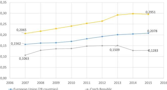
14 EURcent/kWh in 2000 to 29 EURcent/kWh in 2013, see Figure 1 for more details

about the development of prices for households.

Among RES technologies, only large hydropower stations are not dependent on

Figure 1: Prices for households

0,1562

0,2078

0,1063

0,1509 0,1283

0,2065

0,2951

0,00 0,05 0,10 0,15 0,20 0,25 0,30 0,35

2006 2007 2008 2009 2010 2011 2012 2013 2014 2015 2016

European Union (28 countries) Czech Republic

Germany (until 1990 former territory of the FRG)

Eurostat

technology. End customers through so-called EEG levy pay all additional costs associated

with subsidies. In 2000, EEG levy was 0.19 EURcent/kWh and increased to the level of

6.24 EURcent/kWh in 2014. See Figure 2 for more details about the price structure of

German households. The overall cost of EEG subsidies increased drastically during 2009

– 2014, from about EUR 5 billion in 2009 to some EUR 25 billion in 2014. (Poser et al.,

2014).

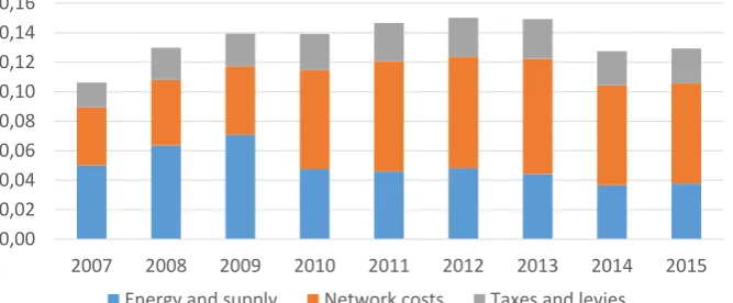
Price structure for Czech households is different. As it can be seen from Figure 3,

taxes and levies account for moreless same portion since 2008. In fact, it slightly increased

from 2.21 EURcent/kWh in 2009 to 2.36 EURcent/kWh in 2015, growth of only 6.8%.

Whereas in Germany for the period from 2009 to 20141 _{growth was 64%. However, the}

surcharge for support of RES went up from 6.7 EUR/MWh in 2010 to 19.8 EUR/MWh

in 20142_{. The development of price structure of Czech households is depicted in Figure 3.}

From 2001 until 2008, amount of feed-in tariffs in Germany went up from some EUR

1.6 billion to EUR 9 billion. With such large amounts of subsidies, only 211.1 million euros

1

Figure 2: German price structure

0,00 0,05 0,10 0,15 0,20 0,25 0,30 0,35

2007 2008 2009 2010 2011 2012 2013 2014

Energy and supply Network costs Taxes and levies

Eurostat

Figure 3: Czech price structure

0,00 0,02 0,04 0,06 0,08 0,10 0,12 0,14 0,16

2007 2008 2009 2010 2011 2012 2013 2014 2015

Energy and supply Network costs Taxes and levies

Eurostat

were allocated to R&D in renewable energies by government, this accounts for 3% of the

have been very successful in aspect of increasing installed capacities of RES. In Germany,

photovoltaics, the recipient of highest FITs, increased its capacity from 100 MW in 2000

to 5311 MW in 2008. In the Czech Republic, installed capacity of PV between 2008 and

2010 soared from 39.5 MW to 1959.1 MW. In addition, Prusa et al. (2013) calculated

that in 2011 average usage of Czech PV plants was only 1099 hours (12.54% of the total

number of hours in the year) and the total cost of PV subsidies was about EUR 972

million and EUR 216 million out of this amount is ”the pure dead weight loss”. Prusa

et al. (2013) define the pure DWL as follows: The pure DWL component is a net loss

to the economy, because it captures the extent of inefficient electricity production. p02 .

The pure DWL is equivalent to an artificial cost which would not exist were it not for the

subsidies. This cost appears because money is invested in PV production capacity that

is more expensive than other feasible sources.

Feed-in tariffs are usually granted for 20 years, this is a good feature for investors,

since they can be assured in long-term support. So even if they would be abolished this

year, additional costs will still be paid for 19 years by end customers, if no retrospective

legislation will be put in force. While, putting retrospective laws in force is a very bad

signal for investors, since they cannot be confident with safety of their investments. In

2010, Czech Republic introduced retroactive legislation in the form of a withholding tax

of 26% for photovoltaics with installed capacity of over 30 kW valid for 2011 – 2013.

Furthermore, Czech government cancelled previously guaranteed tax-free period of first

five years of a project life. The impact was instantaneous, annual installed capacities

of PV plummeted from 1494.5 MW in 2010 to 11.9 MW in 2011, 99.2% decrease in

just one year. Average annual installed capacities for the period 2011 – 2014 is 27.075

MW, furthermore, in 2014 there was even negative installed capacity, i.e. dismantling

of some3 _{PV stations. Moreover, such legislative action of the Czech government also}

indirectly impacted wind sector, in 2011 only 1.1 MW of wind capacity were installed,

whereas in 2010 24.6 MW of wind capacity were installed, 95.5% decrease in just one year.

3

Hydropower also was affected, in 2011 1.5 MW of hydropower capacity were dismantled,

while in 2010 19.6 MW of hydropower capacity were installed, i.e. more than 100%

decrease. Of course we cannot claim, that PV, wind and hydropower sectors declines

were caused solely by the Czech legislative action. For instance, additional reason for

PV sector decline is a stoppage of connections into the grid for new PV plants in 2010,

this problem is more explained in section 3.1.1. Nevertheless, we see that a large drop

in installed capacities occurred next year after Czech government introduced such an

unpopular legislation.

In Germany, FITs for wind farms put in operation in 2003 are expected to be lower

than prices for electricity in 2022 (Frondel et al., 2009). Therefore, it will take 19 years

for wind farms to be competitive without subsidies. It should be mentioned that onshore

wind is considered as moreless mature technology.

Furthermore, technology specific feed-in tariffs reduce competition within RES. If

FITs would have been same for all types of RES, we would not be able to claim that

PV installations would had resulted in same capacities as now. Though in Germany,

installations of PV plant capacities exceed that ones of biomass, biomass has generated

much more energy than solar PV plants. So if subsidies would be the same, it probably

would be more economically reasonable to invest into biomass sector rather than into PV

sector. Prusa et al. (2013) found out that in the Czech Republic, for PV plants to be

non-loss making either prices have to go up seven times or costs have to be reduced seven

times.

Whilst prices for end customers increased, wholesale prices have decreased. In

Ger-many, base load prices plummeted from 90-95 EUR/MWh in 2008 to 37 EUR/MWh in

2013. This created financial problems for utilities that operated thermal power plants.

German utilities companies stocks went down by almost 45 percent from 2010 to 2014

and credit ratings are lowered for them from A to A- or in case of RWE even to BBB+

(Poser et al., 2014).

R&D. Now producers of RES-E are induced to be more cost efficient via degressive rates

of FITs.

Likewise, Menanteau et al. (2003) suggest introduction of ”optimum environmental

tax”. So consumers would be induced to choose between efficient use of energy from

conventional resources or use energy from RES without such tax. So if the cost of

pollution and other environmental damage from conventional production of energy can

be properly estimated such Pigovian tax can be introduced. This would correct the

market imperfections (Menanteau et al., 2003). We know similar tax as tax on CO2

emissions.

2.2

Problems of integrating renewable energy into the grid

One more problem of renewables is grid connection. Producers of RES-E are entitled to

have a priority access into the grid. But locations of some plants are far away from the

grid, for instance offshore wind farms in Germany. So expansion of transmission grids

needs large investments. Investment costs for Germany are estimated to be approximately

EUR 40 billion (Poser et al., 2014) over the decade. There is the ”Grid Development

Plan” in Germany, which encompasses development of infrastructure and connection of

north offshore wind plants with southern regions. In 2012, energy transition induced four

German TSOs to spend EUR 1.15 billion4 _{on network infrastructure.}

In the Czech Republic, the most favourable locations for wind farms are along the

German and Polish borders, as well as Slovakian border and also in the Moravian

high-lands. Accordingly, they are remote from the biggest consumption centers such as Prague,

Ostrava and Brno. Until 2023, Czech TSO is going to invest into expansion of the grid

CZK 60-70 billion5 _{(EUR 2.2 - 2.59 billion; exchange rate is 27) this is the biggest}

in-vestment in the history6 _{of the country. However, this expansion is planned not only}

due to increasing installed capacities of RES but mainly because of increasing capacity

4

https://ec.europa.eu/energy/en/content/2014countryreportsgermany

5

of nuclear power. In contrast with Germany, Czech Republic is not planning to abandon

nuclear power.

In the Czech Republic, in February 2010 due to technical reasons Czech TSO requested

stoppage of connections into the grid for new PV plants. Czech TSO stated that excessive

amount of new PV plants can threaten security of the grid.

For grid operators there are also so-called grid balancing costs. Such costs arise due to

intermittent character of some types of RES. Wind and solar technologies are dependent

on weather, so when there is no wind wind farms do not generate electricity and when

there is a cloudy sky PV plants do not generate electricity. Thus, grid operators must

balance out electricity capacities in the grid in order to prevent stoppages of electricity

supply and security of the grid. Next section discusses intermittency problem more

detailed.

2.3

Intermittent character of renewable energy

Many proponents of RES say that RES will decrease dependency from depleting fossil

fuels. However, RES tend to have intermittent character. For example, onshore wind

farm with installed capacity of 100 MW will produce only 20-35%7 _{of electricity that it}

would have produced if suitable weather conditions were holding all the year round –

this is known as the capacity factor. For solar PV plants, the capacity factor is between

10-20%8_{.In order to save customers from blackouts backup energy systems must be in}

place. In Germany, on January 5, 2012 solar and wind combined production was 500

GWh, maximum for that year; and minimum was on December 19, 2012 with combined

production of only 30 GWh. Therefore, large backup capacities of thermal power plants

must be in place (Poser et al., 2014).

There are different ways to tackle the problem of intermittency, the major ones are:

• _{Use of fossil fuels, so at times when RES-E producers are unable to meet the}

de-7

FS-UNEP, 2016

8

mand, conventional plants start to produce electricity. Maintenance of such systems

is costly. For Germany, amount of EUR 590 million in 2006 was calculated by

Erd-mann (2008). The use of fossil fuels is relatively easy and cheap only in case of

long-term balancing (i.e. days or week notice).

• _{Transmission of surplus from one location to another, this requires good}

intercon-nection between locations. This goes back to the development of the grid and also

may require good collaboration between the states. In addition, it will increase the

grid balancing costs.

• _{Demand response, so when RES expected to produce low volume of electricity, large}

industrial and commercial customers are paid by the grid operator to lower their

consumption of electricity by switching off machines and/or air conditioning etc.

The amount of payment must be properly calculated, nevertheless this method is

costly and difficult to implement. This method is relatively easy to implement in

medium-term notice (i.e. hours).

• _{Energy storage, surplus of produced RES-E is stored and when RES-E producer}

cannot meet the demand stored electricity is fed into the grid. Probably the best

option in short notice (i.e. seconds to minutes).

The latter option is promising because prices for batteries have been falling. For

example, prices of electric vehicle batteries are steadily decreasing. The average cost

per kWh fell from some 1000 $ _{in 2010 (EUR 757.57, exchange rate is 1.32, which is}

average monthly rate for 2010) to some 390 $9 _{in 2015 (EUR 354.55, exchange rate is}

1.10, which is average monthly rate for 2010). The decrease is caused by technological

improvements as well as economies of scale. This is also driven by increasing demand for

electric vehicles. There are two types of storage: so-called ”behind the meter” and the

grid-scale storage.

9

Behind the meter storages are located inside the buildings and reserved for self use.

Germany has a subsidy programme for small-scale PV installations with storage effective

from 2013. By the end of September 2015, 27 000 storage systems were sold with capacity

of 136 MWh10_.

Grid-scale battery storages are of much larger capacities and located close to wind

farms or solar plants. For instance, in Germany 5 MWh storage system was put in

operation for utility which operates a large share of wind energy. In 2015, worldwide

1220 MW11 of grid-scale projects were announced.

Nonetheless, the storage systems increase the costs of RES-E. In 2015, German

lev-elised cost of electricity for onshore wind farm with storage of 50% of total installed

capacity is 120 $_/MWh12 _{(EUR 109.09, exchange rate is 1.10), which is 48% higher than}

without storage capacity. For PV plants such cost is 198 $_/MWh13 _{(EUR 180, exchange}

rate is 1.10), which is 85% higher than without storage. Consequently, we see that storage

systems increase the costs substantially, yet these costs tend to decrease, since prices for

batteries decrease and overall development of storage technology is promising.

In addition, wholesale prices have become dependent on weather conditions.

Whole-sale prices go down when the sun shines and the wind is strong and go up when no wind

and no sun but high demand for power remains. Therefore, price forecasts for futures

have become more subtle and complicated.

2.4

Reduced CO2 emissions

Prices of CO2 emission certificates, which are traded on European Emissions Trading

System (ETS), have never been above 30 EUR/tonne of CO2. In 2008, calculated cost

of abatement one tonne of CO2 emission by PV in Germany was 716 euros and by wind

energy was 54 euros (Frondel et al., 2009). Therefore, from economic point of view it is

10

See prev. note

11

See prev. note

12

See prev. note

13

much more beneficial to buy certificates than subsidize renewable energies.

Nevertheless, in 2009, about 340 million metric tonnes of CO2 emissions were saved

by the use of RES in EU. Taking the price of 15 EUR/tonne of CO2 in 2009, savings will

result in EUR 51 billion for 2009 year alone (Poser et al., 2014).

In order to see correlation between change in RES share in gross final energy

con-sumption and greenhouse gas (hereinafter GHG) abatement for Germany we will run the

following regressions14

GHGE = β0 +β1RESE

GHGHC = β0 +β1RESHC

GHGT = β0 +β1REST

where, GHGE = GHGEt−GHGEt₋₁, i.e. yearly change in amount of GHG

abate-ment induced by change in RES-E share in gross final electricity consumption; and

RESE = RESEt −RESEt₋₁, i.e. yearly change of RES-E share in gross final

elec-tricity consumption. Analogously, other two regressions should be read. Likewise, all

three regressions were tested for heteroskedasticity (hettest), normality (swilk) and

spec-ification test for omitted variables (ovtest) results can be found in Appendix A in notes

under the relevant table.

No regressions were run for the Czech Republic due to lack of data.

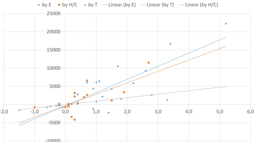
Figure 4 is a scatter plot for all three regressions. Y-axis is measured in tonnes of CO2

equivalent and X-axis is measured in percentage points. Regression of GHG abatement

by RES-E resulted in R-squared of 0.5653, i.e. 56.53% of variability in dependent variable

is explained by the independent one. Likewise, equation of the regression – a blue line –

14

Figure 4: GHG abatement by different types of RES

-10000 -5000 0 5000 10000 15000 20000 25000

-2,0 -1,0 0,0 1,0 2,0 3,0 4,0 5,0 6,0

by E by H/C by T Linear (by E) Linear (by T) Linear (by H/C)

is:

\

GHGE=−317.18

(1820.415) + 3609(845..₇₉₎046RESE

Coefficient is statistically significant even at 1% significance level. Thus, one percent

increase of RES-E share in gross final electricity consumption results in abatement of

3609.046 tonnes of CO2 equivalent. Constant in this regression is statistically

insignifi-cant.

Regression of GHG abatement by RES-H/C has R-squared of 0.5113. Equation of

the regression line – an orange line – is:

\

GHGHC =−290.5662

(818.₁₄₎

+ 3132.254

(818.3969)RESHC

Constant is statistically insignificant, whereas coefficient is statistically significant even

at 1% significance level. Therefore, when RES-H/C share in final energy consumption in

CO2 equivalent.

Regression of GHG abatement by RES-T has R-squared of 0.9851, which is almost

perfect correlation. Equation of the regression line – a grey line – is:

\

GHGT =−6.637

(31.₂₆₎

+ 951.2398

(31.3) REST

Here constant is also statistically insignificant and coefficient is statistically significant

even 1% significance level. Thus, 1% increase in RES-T share energy consumption in

transport increases GHG abatement by 951.239 tonnes of CO2 equivalent.

Having these results and estimations of RES shares from Table 2.2 we can estimate

the amount of GHG abatement in 2020 by multiplication of relevant coefficients with

estimated shares of relevant RES. Thereby, we have the following estimations:

RES −E₂₀₂₀xcoef.RESE = 139309.2

RES −H/C₂₀₂₀xcoef.RESHC = 48549.94

RES −T₂₀₂₀xcoef.REST = 12556.37

All estimations are measured in tonnes of CO2 equivalent. Thus, we have that in

2020 year alone total estimated GHG abatement is 200 415.5 thousand tonnes of CO2

equivalent, according to German NREAP 215 million tonnes of CO2 equivalent will be

prevented by 2020, thus there is less than 7% discrepancy between my estimations and

German NREAP estimations. Taking into account that prices of certificates on ETS

should increase, savings in money equivalent will be significant. If we take current price15

of EU Emission Allowance – 6.05 EUR per tonne of CO2 equivalent, we can estimate

that savings in 2020 year alone will be 1.213 billion EUR. However, these estimation is

assuming that prices will remain at its current level, whereas they must go up, since the

15

number of the certificates will gradually go down. This estimation is conducted in order

to show you the size effect of GHG abatement.

3

Installed renewable capacity and feed-in tariffs

3.1

Model

We are going to analyse dependence between feed-in tariffs and installed capacity of each

type of RES-E in Germany and the Czech Republic via linear regression. Firstly, we will

use simple linear regression, our dependent variable will be installed capacity in year t,

M Wt, and independent variable will be FIT in year t, F ITt. Thus, the equation will be:

M Wt=β₀ +β₁F ITt

Then for some types of RES we will add polynomial of second order and in two cases

polynomial of third order, in case of Czech solar RES we will add a polynomial of fourth

order and a dummy, reasoning will be explained later. Therefore the equations will be:

M Wt =β₀+β₁F ITt2 +β2F ITt

M Wt=β₀+β₁F ITt3+β2F IT

2

t +β3F ITt

M Wt=β0+β1F ITt4+β2F IT

3

t +β3F IT

2

t +β4F ITt+β5D

All successful regressions (i.e. p-value of F-test is lower than 0.05 or in some cases lower

than 0.1) were tested for heteroskedasticity (hettest), normality (swilk) and specification

test for omitted variables (ovtest) results can be found in Appendix A in notes under the

relevant table.

For Germany data will be taken between years 2000 and 2015. However, if value of

F ITt for some t is zero, then this year is omitted. There are such cases in landfill, sewage

were introduced also in 2004, and in offshore wind RES, where FITs were introduced in

2009. The data for Germany is taken from Federal Ministry for Economic Affairs and

Energy. It should be mentioned that each technology-specific average FIT for a given

year will be used as F ITt.

For the Czech Republic data will be taken for 2002 – 2015 period. No restrictions on

value of F ITt are imposed. Nevertheless, for the Czech Republic we managed to collect

much less data than for Germany. We could not find data about installations of biomass

and biogas16 RES. The data for the Czech Republic is taken from the Energy Regulatory

Office.

3.2

Results of the model

Regression for German hydropower resulted in statistically insignificant coefficient of

F IT, p-value of the coefficient is 0.543. In addition, R-squared is only 0.0271, which

means that only 2.71% of variability in dependent variable is explained by the independent

one. Finally, regression itself is insignificant, since p-value of the F-test is 0.5426. This

is caused by the fact that sites for such RES technology are scarce, since can be located

only on rivers. Therefore, there is no relation between the size of FIT and installation

amounts. Average annual growth rate of installed capacity for the period of 2001 – 2015

is 0.99%. It should be noted, that hydropower is the most mature type of RES among

all, since it has been developing for decades.

Regression for Czech hydropower also resulted in statistically insignificant coefficient

of F IT, p-value of the coefficient is 0.585. R-squared of the regression is only 0.0527.

This is caused by the same reasons as in German case.

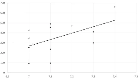
Figure 5 is a scatter plot for German landfill, sewage and mine gas RES. Y-axis is

the amount of annual installed capacity of this RES in MW. X-axis is a feed-in tariff in

16

Figure 5: German landfill, sewage and mine gas

0 100 200 300 400 500 600 700

6,9 7 7,1 7,2 7,3 7,4 7,5

BMWi and own computations

EURcent/kWh. Equation of the line is:

[

M W = −4239

(2325.₇₉₎

+ 643.87

(325.99)F IT

Thus, one cent of FIT corresponds to 643.87 MW of installed capacity. For instance, if in

year t+1 FIT will be increased by one cent, then installed capacity will be increased by

643.87 MW in comparison to year t. p-value of the coefficient is 0.07617_{, i.e. coefficient}

is statistically significant at 10% significance level. Likewise, overall significance of the

regression is achieved only at 10% significance level, since p-value of the F-test is 0.0765.

In addition, so far maximum change of FIT was 0.2 cent, increase in 2011 from 7.2 to 7.4

and decrease in 2013 from 7.3 to 7.1. R-squared of this equation is 0.2806, i.e. independent

variable explains 28.06% of variability of dependent variable. Though, average growth

rate of FIT between 2005 and 2015 is only 0.14%, average annual growth rate of installed

capacity is 20.97%.

17

No regression was run for the Czech Republic due to lack of data.

Geothermal type of RES started to develop in Germany in 2007, when the first 2 MW

of this type of RES were installed. Average growth rate of installed capacity is 55%,

nonetheless there were years with no increase at all and years such as 2012, when 13 MW

were added, resulting in 260% increase in comparison to 2011. Regression resulted in

statistically insignificant coefficient and constant, with p-values 0.34 and 0.55 respectively.

Moreover, overall regression is insignificant, p-value of the F-test is 0.3396. This is caused

by scarcity of this type of RES, i.e. special site needed to be found in order to generate

geothermal energy. Therefore, feed-in tariffs do not impact amount of installed capacity

of this type of RES.

No regression was run for the Czech Republic due to lack of data.

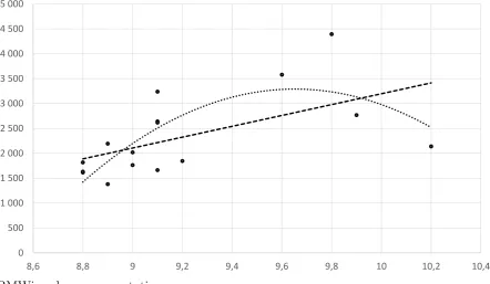
Figure 6: German onshore wind

0 500 1 000 1 500 2 000 2 500 3 000 3 500 4 000 4 500 5 000

8,6 8,8 9 9,2 9,4 9,6 9,8 10 10,2 10,4

BMWi and own computations

Figure 6 is a scatter plot for German onshore wind RES. Y-axis and X-axis are same

as in Figure 5. Equation of the dashed line is

Therefore, one cent of FIT corresponds to 1090 MW of installed capacity. For instance,

if in year t+1 FIT will be increased by one cent, then installed capacity in year t+1

will be increased by 1090 MW in comparison to year t. R-squared of this equation is

0.3208, i.e. independent variable explains 32.08% of variability of dependent variable.

p-value of independent variable is 0.022, i.e. it is statistically significant at 5%

signif-icance level, whereas, p-value of constant is 0.069, i.e. it is not statistically significant

at 5% significance level, however at 10% significance level it is statistically significant.

But, Breusch-Pagan test for heteroskedasticity yields that there is a constant variance18.

Nevertheless, when we add in the model a polynomial of the second order, Breusch-Pagan

test for heteroskedasticity rejects null hypothesis, which is constant variance of dependent

variable fitted values. Likewise, R-squared increases to the level of 0.5525, all coefficients

and constant are statistically significant at 5% significance level. The equation of this

model – dotted line – is:

[

M W =−2570.459

(991.01) F IT

2_{+ 49620.89} (18714.₀₃₎F IT

−236183.6

(88148.₇₂₎

By calculating the maximum of this parabola we find the optimum FIT for onshore

wind RES, i.e. under this FIT the maximum annual installed capacity is anticipated.

The optimum FIT is 9.65 EURcent/kWh. Therefore, higher FITs are inefficient, since

they result in lower installed capacities at higher expenses. Likewise, FITs below 8.52 will

result in negative installed capacities. Therefore, FITs should be set inside (8.52;9.65]

interval. In addition, average growth rate of FIT is only 0.40% for the period of 2001 –

2015, average installed capacity growth rate is 14.16%.

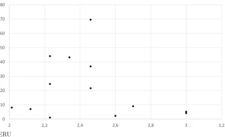
Figure 7 is a scatterplot for Czech wind RES. Y-axis is in MW of installed capacity and

X-axis is a feed-in tariff in CZK/kWh. I have run various regressions: simple ones, with

polynomials of the second, third and even fourth orders. No regression was successful. It

is seen from Figure 7 that data is very dispersed, thus very difficult to draw a line which

18

Figure 7: Czech wind

0 10 20 30 40 50 60 70 80

2 2,2 2,4 2,6 2,8 3 3,2

ERU

would approximately match the pattern. In all regressions, overall p-values were greater

than 0.1706. Thus, we can conclude that wind installations are independent from FITs.

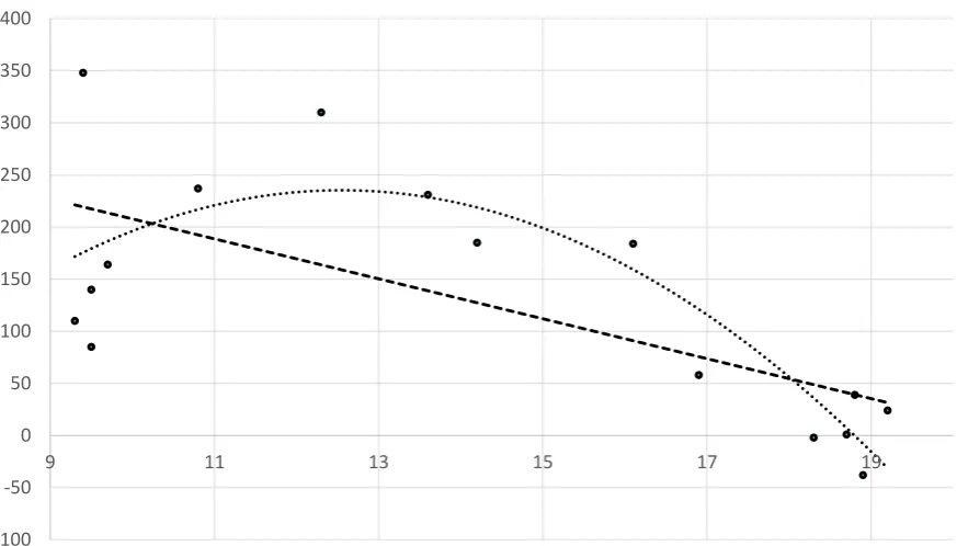
Figure 8: German offshore wind

-500 0 500 1 000 1 500 2 000 2 500

14,5 15 15,5 16 16,5 17 17,5 18 18,5 19

Figure 8 is a scatter plot for offshore wind RES in Germany. Y-axis and X-axis are

same as in Figure 5. Equation of the dashed line is

[

M W =−6702.93

(2616.₇₇₅₎

+ 438.46

(159.46)F ITt

Hence, one cent of FIT corresponds to 438.46 MW of installed capacity. For instance, if

in year t+1 FIT will be increased by one cent, then installed capacity will be increased by

438.46 MW in comparison to year t. R-squared of this equation is 0.6019, i.e. independent

variable explains 60.19% of variability of dependent variable. Independent variable is

statistically significant at 5% significance level, p-value of constant is 0.051, i.e. constant

is almost statistically significant at 5% significance level. Yet, Ramsey RESET test

concludes that we have omitted variables19_{. Accordingly, when we add in the model a}

polynomial of second order, R-squared of the model increases to the level of 0.9910, i.e.

model explains 99.1% of variability in the dependent variable. In addition, all coefficients

and constant are statistically significant even at 1% significance level. The equation of

the model – dotted line – is:

[

M W = 353.0522

(26.86775)F IT

2_−11207.84

(886.7051)F IT + 88725(7275.592).89

The minimum corresponds to the point where derivative changes its sign, i.e. negative

marginal returns change to increasing marginal returns. The minimum here is 15.8727,

parabola at this point is below zero, i.e. when FIT is set at 15.8727 annual installed

capacity will be negative. So producers of RES will dismantle their wind farms. Actually,

parabola is negative when values of FIT are inside [15.0764;16.6691] interval. Therefore,

FITs should not be set inside this interval. However, such model implies that FIT set at

0 will result in 88725.89 MW of installed capacity, which is barely can make sense. In

order to exclude this shortcoming of the model, we add a polynomial of third order, and

19

now the model – wide dashed line – is:

[

M W = 9

(24.15052)9.41284F IT

3_−4656.334 (1216.998)F IT

2_{+ 72632.58} (20371.35)F IT

− 377268

(113251.5)

All coefficients and constant are statistically significant at 5% significance level.

R-squared increased a little bit to the level of 0.9986. There are two points where derivative

is zero: 15.1436 and 16.082. Inside the interval of these two values marginal returns

are negative. Therefore it is inefficient to set FITs inside this interval. In addition,

FITs set below 14.5612 result in negative installed capacities. Accordingly, FITs should

be set inside the intervals (14.5612;15.1436] and (16.5519; +∞). We excluded interval

(16.082;16.5519) because FITs set inside [14.6736;15.1436] interval result in same installed

capacities but with lower FITs.

First offshore wind farms in Germany were installed in 2009, with 30 MW. Ever since,

the average annual growth rate of installed capacity is 126%. Offshore wind projects are

very expensive, since they have excessive initial investment costs. And the project makes

sense only if it is of bigger scale, that is why we see such big growth rates of installed

capacities. This type of RES showed incredible growth, with only 30 MW installed in

2009, 3283 MW were installed in 2015 alone. Growth of more than 10 000 % in 6 years.

Figure 9 is a scatter plot for biomass RES. Y-axis and X-axis are same as in Figure 5.

Equation of the dotted line is

[

M W = 399.44

(82.6653)

−19.16

(5.66)F ITt

That is, one cent of FIT corresponds to decrease of 19.16 MW of installed capacity.

For instance, if in year t+1 FIT will be increased by one cent, then installed capacity

will be decreased by 19.16 MW in comparison to year t. Constant and independent

variables are statistically significant at 5% significance level. R-squared of this equation

Figure 9: German biomass

-100 -50 0 50 100 150 200 250 300 350 400

9 11 13 15 17 19

BMWi and own computations

0.6808. Coefficients remain statistically significant at 5% significance level, but p-value of

constant is 0.075, thus constant is statistically significant only at 10% significance level.

The equation of the model – dotted line – is:

[

M W =−6.027

(1.966) F IT

2_{+ 151.2494} (55.₇₇₉₈₂₎F IT

−713.6272

(368.₉₉₆₆₎

The maximum of the parabola is the optimum FIT, i.e. maximum annual installed

capacity is achieved under this FIT. The maximum is at 12.5476, consequently FITs

higher than 12.5476 are inefficient, since they will result in lower installed capacities

at higher costs. In addition, FITs set below 6.29957 will result in negative installed

capacities. Therefore, FITs should be set inside (6.29957;12.5476] interval. Average

growth rate of FIT between 2001 and 2015 is 5% and average annual growth rate of

installed capacity is 16%. Nevertheless, in recent years the growth slowed down to average

of 0.62%20_{. The boom of installations of this type of RES was between 2001 and 2006}

20

with average annual growth rate of 33%.

No regression was run for the Czech Republic due to lack of data.

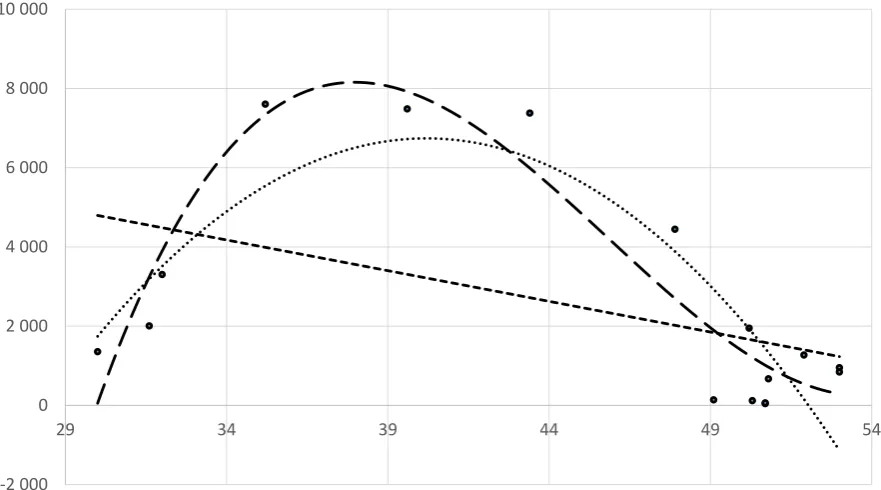
Figure 10: German solar energy

-2 000 0 2 000 4 000 6 000 8 000 10 000

29 34 39 44 49 54

BMWi and own computations

Figure 10 is a scatter plot for solar RES in Germany. Y-axis and X-axis are same as

in Figure 5. Equation of the line is

[

M W = 9441.76

(3542.₄₈₄₎

−154.9

(77.₅₃₎F IT t

Constant is statistically significant at 5% significance level and independent variable is

statistically significant only at 10% significance level as well as whole regression is

signifi-cant only at 10% significance level. R-squared of this equation is 0.2219, i.e. independent

variable explains 22.19% of variability of dependent variable. With one cent increase in

FIT, installed capacity will decrease by 154.9 MW. But, Ramsey RESET test concludes

that we have omitted variables. Thence, we add a polynomial of second order. All

co-efficients and constant become statistically significant even at 1% significance level and

level of 0.7148. The equation of the model – dotted line – is:

[

M W =−48.062F IT

(10.₁₃₈₎

2_{+ 3863.828} (849.1176)F IT

−70916.21

(17096.32)

The optimum FIT for this model is where parabola has its maximum. The maximum

is at 40.1963, consequently, FITs higher than 40.1963 are inefficient. Furthermore, FITs

set below 28.3546 result in negative installed capacities. Therefore, FITs should be set

inside (28.3546;40.1963] interval. Yet, Ramsey RESET test still concludes that we have

omitted variables. Thus, we add polynomial of third order and Ramsey RESET test does

not conclude that we have omitted variables. It slightly changes our intervals. Likewise,

R-squared increases to the level of 0.8531, all coefficients and constant remain statistically

significant at 1% significance level. The equation of the model – wide dashed line – is:

[

M W = 4.0298

(1.₁₉₈₈₅₎F IT

3_−554.4399 (150.₈₃₆₇₎F IT

2_{+ 24675.01} (6223.₆₈₅₎F IT

− 350005

(84994.₆₁₎

There are two points where derivative is zero: 37.9719 and 53.7514. Inside the

inter-val of these inter-values marginal returns are negative, thus, it is inefficient to set FIT

be-tween 37.9719 and 53.7514. In addition, FITs set below 29.9764 will result in

nega-tive installed capacities. Therefore, FITs should be set inside the following intervals:

(29.9764;37.9719] and (61.6409; +∞). We excluded interval (53.7514; 61.6409), since

val-ues inside [30.0824;37.9719] result in the same installed capacities but at lower FITs.

This is the only type of RES for which average FIT has been steadily decreasing since

2006, average decrease rate of 5% between years 2006 and 2015. Nonetheless, average

annual installed capacity growth rate for the same period is 16%, with boom in 2009

with 128% annual growth rate. Moreover, now there are 3 consecutive years of negative

annual growth rates of installed capacity.

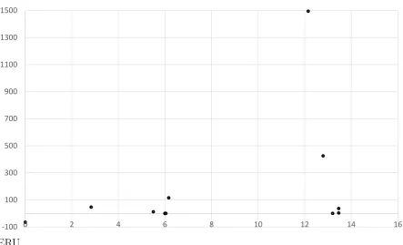
Figure 11 is a scatter plot for Czech solar energy. Y-axis and X-axis are same as

in Figure 7. As it has already been written, in 2010 Czech government introduced a

Figure 11: Czech solar energy

-100 100 300 500 700 900 1100 1300 1500

0 2 4 6 8 10 12 14 16

ERU

there was an unexpected boom of photovoltaic installations, which led to stoppage of

connections into the grid for new PV installations. That is why, I added a dummy

variable ”D”, which was equal 1 only for 2010 year and 0 for all others years. Only after

adding polynomial of fourth order regression was moreless successful. Ramsey RESET

test still concluded that there is an omitted variable, though at 4% significance level

did not. Breusch-Pagan test for heteroskedasticity did not detect any heteroskedasticity.

Regression equation is:

[

M W = −0.698

(0.1704983)F IT

4_{+ 16.12} (4.₂₉₈₎F IT

3 _−107.27 (35.₀₃₉₎F IT

2_{+ 228.829}

(101.₄₉₁₉₎F IT + 913₍₁₃₇.₉₈₄₎.9D

−64.49

(74.₃₂₎

Constant here is statistically insignificant. Function for FITs has three values where

derivatives are zero: 1.57; 4.72; 11.026. Inside (1.57;4.72) interval marginal returns are

negative, i.e. it is inefficient to set FITs inside this interval. Inside [4.72;11.026) marginal

returns are positive. However, FITs should be set inside the following intervals: (0;1.57]

result in same installed capacities.

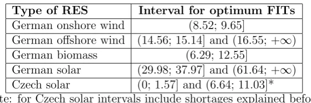
Table 1: Summary of optimal FITs

Type of RES Interval for optimum FITs

German onshore wind (8.52; 9.65]

German offshore wind (14.56; 15.14] and (16.55; +∞) German biomass (6.29; 12.55]

German solar (29.98; 37.97] and (61.64; +∞) Czech solar (0; 1.57] and (6.64; 11.03]*

Note: for Czech solar intervals include shortages explained before.

Table 1 summarizes all found optimum intervals for feed-in tariffs. We did not find

optimum intervals for FITs in cases of: hydro RES of both countries, landfill,sewage and

mine gas RES of both countries, Czech wind RES and Czech biomass. Moreover, optimum

interval of FITs for Czech solar includes some shortages explained before. Therefore, we

have optimum intervals for FITs in 5 cases. Thereby, we believe that if feed-in tariff

scheme to be continued and governments want to maximize their installed capacities

of RES, they should set feed-in tariffs inside these intervals. For Germany, FITs are

measured in euros and for the Czech Republic FITs are measured in Czech korunas.

4

Conclusion

The main purpose of this paper was to determine what are the growth opportunities of

renewable energy and how renewable energy is financed in the Czech Republic and

Ger-many. After reviewing German and Czech renewables policies we conclude that support

for renewable energy is mainly covered by end-customers. End-customers of both

coun-tries have additional costs related to support of RES included in their bills. Additional

costs related to RES include: feed-in tariffs and other financial types of support, grid

development costs and grid balancing costs. All these costs are firstly borne by TSOs

and DSOs but then they are passed onto end-customers. However, not all additional

costs are borne by end-customers, in the Czech Republic, there is a subsidy, which covers

some tax benefits. This support resulted in significant increase of installed capacities in

all types of RES excluding hydro, since it has already been very developed. However,

since feed-in tariff scheme is regarded as a very costly method and moreover, European

Commission has approved the removal of all feed-in tariff schemes from 2017, Germany

has already started to shift towards auction scheme.

Various shortcomings related to renewables are discussed and some ways of how to

resolve these shortcomings are provided. We estimated relation between GHG abatement

and share of RES. We also analyse the dependence between annual installed capacities

of RES and respective feed-in tariffs. We took the empirical data of annual installed

capacities and regressed it on respective FITs and/or their polynomials. The analysis

resulted in optimum intervals for some types of RES, they are summarised in our paper.

We could not collect most of the data for the Czech Republic, since the Energy Regulatory

Office of the Czech Republic does not publish the time series for RES, unlike Germany,

which publishes a comprehensive database regarding RES.

Optimum intervals in our paper indicate at which values of FIT the biggest amount of

installed capacities is anticipated. Thus, if FIT schemes are to be continued after 2017,

FITs should be set inside these intervals. These intervals assume that there are not any

caps and restrictions. Nonetheless, there were regressions with statistially insignificant

results, for instance, hydro RES in Germany and the Czech Republic. In this case, we

conclude that size of FITs do not really plays a big role in decision making of investors,

i.e. investors are more concerned about other factors rather than about FITs. Likewise,

Bibliography

• Erdmann_{, G. (2008): “Indirekte Kosten der EEG-Foerderung. Kurz-Studie im}

Auftrag der WirtschaftsVereinigungMetalle”Technische Universitaet Berlin

• Frondel_{, M., N.} Ritter_{, C. M.} Schmidt _{& C.} Vance _{(2010): “Economic}

im-pacts from the promotion of renewable energy technologies: The German

experi-ence.” Energy Policy 38: pp. 4048–4056.

• IRENA and CEM _{(2015): “Renewable Energy Auctions – A Guide to Design.”}

• Jirous_{, F., (2011): “Integration of electricity from renewables to the electricity}

grid and the electricity market – RES – Integration. National report: Czech

Re-public”eclareon

• Menanteau_{, P., D.} Finon_{& M.} Lamy _{(2003): “Prices versus quantities:}

choos-ing policies for promotchoos-ing the development of renewable energy”Energy Policy 31: pp. 799–812.

• Poser_{, H., J.} Altman_{, F.} ab Egg_{, A.} Granata _{& R.} Board _(2014):

“De-velopment and integration of renewable energy: lessons learned from Germany”

Finadvice

• Prusa_{, J., A.} Klimesova _{& K.} Janda _{(2013): “Consumer loss in Czech}

Appendix A – Regression Outputs

Table 2: Stata output for German GHG abatement by RES-E

Source SS df MS Number of obs 16

F( 1, 14) 18.21 Model 3.54E+08 1 3.5E+08 Prob>F 0.0008 Residual 2.72E+08 14 1.9E+07 R-squared 0.5653

Adj R-squared 0.5343 Total 6.27E+08 15 4.2E+07 Root MSE 4410.9 GHGEDE Coef. Std. Err. t P>t [95% Conf. Interval] RESEshareDE 3609.046 845.7903 4.27 0.001 1795.007 5423.086 cons -317.18 1820.415 -0.17 0.864 -4221.58 3587.222

Note: ovtest Prob >F = 0.7104; hettest Prob >chi2 = 0.1165; swilk Prob >Z = 0.0911

Table 3: Stata output for German GHG abatement by RES-H/C

Source SS df MS Number of obs 16

F( 1, 14) 14.65 Model 1.08E+08 1 1.1E+08 Prob >F 0.0018 Residual 1.04E+08 14 7393880 R-squared 0.5113

Adj R-squared 0.4764 Total 2.12E+08 15 1.4E+07 Root MSE 2719.2 GHGHCDE Coef. Std. Err. t P>t [95% Conf. Interval] RESHCshareDE 3132.254 818.3969 3.83 0.002 1376.967 4887.541 cons -290.566 818.1411 -0.36 0.728 -2045.3 1464.172

Table 4: Stata output for German GHG abatement by RES-H/C

Source SS df MS Number of obs 16

F( 1, 14) 923.55 Model 13027681 1 1.3E+07 Prob >F 0 Residual 197484.9 14 14106.1 R-squared 0.9851

Adj R-squared 0.984 Total 13225166 15 881678 Root MSE 118.77 GHGTDE Coef. Std. Err. t P>t [95% Conf. Interval] RESTshareDE 951.2398 31.30108 30.39 0 884.1057 1018.374 cons -6.63744 31.26193 -0.21 0.835 -73.6876 60.41274

Note: ovtest Prob >F = 0.3923; hettest Prob >chi2 = 0.9475; swilk Prob >Z = 0.13027

Table 5: Stata output of German regression for hydro RES

Source SS df MS Number of obs 16

F( 1, 14) 0.39 Model 4526.865 1 4526.865 Prob>F 0.5426 Residual 162676.1 14 11619.72 R-squared 0.0271

Adj R-squared -0.0424 Total 167202.9 15 11146.86 Root MSE 107.79 MWHydroDE Coef. Std. Err. t P>t [95% Conf. Interval] FITHydroDE -18.1088 29.01279 -0.62 0.543 -80.33507 44.11741 cons 211.4045 236.0032 0.90 0.386 -294.7721 717.5811

Note: no tests were done, since regression is insignificant.

Table 6: Stata output of Czech regression for hydro RES

Source SS df MS Number of obs 8

F( 1, 6) 0.33 Model 41.81111 1 41.81111 Prob>F 0.5845 Residual 751.9777 6 125.3296 R-squared 0.0527

Adj R-squared -0.1052 Total 793.7888 7 113.3984 Root MSE 11.195 MWhydroCZ Coef. Std. Err. t P>t [95% Conf. Interval] FIThydroCZ 7.676342 13.29032 0.58 0.585 -24.84389 40.19658 cons -15.9082 38.97599 -0.41 0.697 -111.279 79.46259

Table 7: Stata output of German regression for landfill, sewage and mine gas RES

Source SS df MS Number of obs 12

F( 1, 10) 3.9 Model 85677.72 1 85677.72 Prob >F 0.0765 Residual 219624 10 21962.4 R-squared 0.2806

Adj R-squared 0.2087 Total 305301.7 11 27754.7 Root MSE 148.2 MWlandfillDE Coef. Std. Err. t P>t [95% Conf. Interval] FITlandfil∼E 643.8705 325.9901 1.98 0.076 -82.48075 1370.222 cons -4239.11 2325.79 -1.82 0.098 -9421.292 943.0728

Note: ovtest Prob >F = 0.6085; hettest Prob >chi2 = 0.8844; swilk Prob >Z = 0.18622

Table 8: Stata output of German regression for geothermal RES

Source SS df MS Number of obs 12

F( 1, 10) 1.01 Model 15.53274 1 15.53274 Prob>F 0.3396 Residual 154.4673 10 15.44673 R-squared 0.0914

Adj R-squared 0.0005 Total 170 11 15.45455 Root MSE 3.9302 MWgeoDE Coef. Std. Err. t P>t [95% Conf. Interval] FITgeoDE 0.282413 .2816304 1.00 0.34 -0.3450982 0.909925 cons -3.40822 5.511267 -0.62 0.55 -15.68808 8.871653

Note: no tests were done, since regression is insignificant.

Table 9: Stata output of German regression for onshore wind RES

Source SS df MS Number of obs 16

F( 1, 14) 6.61 Model 3314183 1 3314183 Prob >F 0.0222 Residual 7015292 14 501092.3 R-squared 0.3208

Adj R-squared 0.2723 Total 10329475 15 688631.7 Root MSE 707.88 MWonshoreDE Coef. Std. Err. t P>t [95% Conf. Interval] FITonshoreDE 1090.021 423.8435 2.57 0.022 180.9671 1999.075 cons -7703.76 3906.02 -1.97 0.069 -16081.33 673.8246

Table 10: Stata output of German regression for onshore wind RES with polynomial of 2nd order

Source SS df MS Number of obs 16

F( 2, 13) 8.02 Model 5706569 2 2853284 Prob >F 0.0054 Residual 4622906 13 355608.2 R-squared 0.5525

Adj R-squared 0.4836 Total 10329475 15 688631.7 Root MSE 596.33 MWonshoreDE Coef. Std. Err. t P>t [95% Conf. Interval] FITonshoreDE 49620.89 18714.03 2.65 0.02 9191.685 90050.1 FITonshore∼q -2570.46 991.0165 -2.59 0.022 -4711.42 -429.498

cons -236184 88149.72 -2.68 0.019 -426620 -45747.7 Note: ovtest Prob >F = 0.2548; hettest Prob >chi2 = 0.0984;

swilk Prob >Z = 0.80035

Table 11: Stata output of German regression for offshore wind RES

Source SS df MS Number of obs 7

F( 1, 5) 7.56 Model 2325630 1 2325630 Prob >F 0.0403 Residual 1538064 5 307612.9 R-squared 0.6019

Adj R-squared 0.5223 Total 3863694 6 643949 Root MSE 554.63 MWoffshoreDE Coef. Std. Err. t P>t [95% Conf. Interval] FIToffshor∼E 438.4589 159.4633 2.75 0.04 28.54531 848.3724 cons -6702.93 2616.775 -2.56 0.051 -13429.57 23.69948

Note: ovtest Prob >F = 0.0027; hettest Prob >chi2 = 0.0994; swilk Prob >Z = 0.29774

Table 12: Stata output of German regression for offshore wind RES with polynomial of 2nd order

Source SS df MS Number of obs 7

F( 2, 4) 219.9 Model 3828870 2 1914435 Prob >F 0.0001 Residual 34823.56 4 8705.889 R-squared 0.991

Adj R-squared 0.9865 Total 3863694 6 643949 Root MSE 93.305 MWoffshoreDE Coef. Std. Err. t P>t [95% Conf. Interval] FIToffshor∼E -11207.8 886.7051 -12.64 0 -13669.7 -8745.96 FIToffshor∼q 353.0522 26.86775 13.14 0 278.4554 427.649

cons 88725.89 7275.592 12.20 0 68525.61 108926.2 Note: ovtest Prob >F = 0.1291; hettest Prob >chi2 = 0.5067;

Table 13: Stata output of German regression for offshore wind RES with polynomial of 3rd order

Source SS df MS Number of obs 7

F( 3, 3) 736.62 Model 3858456 3 1286152 Prob >F 0.0001 Residual 5238.035 3 1746.012 R-squared 0.9986

Adj R-squared 0.9973 Total 3863694 6 643949 Root MSE 41.785 MWoffshoreDE Coef. Std. Err. t P>t [95% Conf. Interval] FIToffshor∼E 72632.58 20371.35 3.57 0.038 7801.834 137463.3 FIToffshor∼q -4656.33 1216.998 -3.83 0.031 -8529.36 -783.305 FIToffshor∼u 99.41284 24.15052 4.12 0.026 22.55512 176.2706

cons -377268 113251.5 -3.33 0.045 -737685 -16851.2 Note: ovtest Prob >F = 0.5667; hettest Prob >chi2 = 0.5080;

swilk Prob >Z = 0.65274

Table 14: Stata output of German regression for biomass RES

Source SS df MS Number of obs 16

F( 1, 14) 11.46 Model 89203.11 1 89203.11 Prob >F 0.0044 Residual 108981.9 14 7784.421 R-squared 0.4501

Adj R-squared 0.4108 Total 198185 15 13212.33 Root MSE 88.229 MWbiomassDE Coef. Std. Err. t P>t [95% Conf. Interval] FITbiomassDE -19.1608 5.660266 -3.39 0.004 -31.30086 -7.02074 cons 399.4383 82.66532 4.83 0 222.1388 576.7378

Note: ovtest Prob >F = 0.0544; hettest Prob >chi2 = 0.1122; swilk Prob >Z = 0.61289

Table 15: Stata output of German regression for biomass RES with polynomial of 2nd order

Source SS df MS Number of obs 16

F( 2, 13) 13.86 Model 134919.1 2 67459.55 Prob >F 0.0006 Residual 63265.91 13 4866.608 R-squared 0.6808

Adj R-squared 0.6317 Total 198185 15 13212.33 Root MSE 69.761 MWbiomassDE Coef. Std. Err. t P>t [95% Conf. Interval] FITbiomassDE 151.2494 55.77982 2.71 0.018 30.74439 271.7543 FITbiomass∼q -6.02677 1.966364 -3.06 0.009 -10.2748 -1.7787

Table 16: Stata output of German regression for solar RES

Source SS df MS Number of obs 16

F( 1, 14) 3.99 Model 25337064 1 25337064 Prob >F 0.0655 Residual 88859997 14 6347143 R-squared 0.2219

Adj R-squared 0.1663 Total 1.14E+08 15 7613137 Root MSE 2519.4 MWpvDE Coef. Std. Err. t P>t [95% Conf. Interval] FITPVDE -154.907 77.53224 -2.00 0.066 -321.1972 11.38301 cons 9441.761 3542.484 2.67 0.018 1843.888 17039.63

Note: ovtest Prob >F = 0.0000; hettest Prob >chi2 = 0.0711; swilk Prob >Z = 0.05059

Table 17: Stata output of German regression for solar RES with poly-nomial of 2nd order

Source SS df MS Number of obs 16

F( 2, 13) 16.29 Model 81632652 2 40816326 Prob >F 0.0003 Residual 32564409 13 2504955 R-squared 0.7148

Adj R-squared 0.671 Total 1.14E+08 15 7613137 Root MSE 1582.7 MWpvDE Coef. Std. Err. t P>t [95% Conf. Interval] FITPVDE 3863.828 849.1176 4.55 0.001 2029.421 5698.235 FITpvDEsq -48.0617 10.13821 -4.74 0 -69.9639 -26.1594

cons -70916.2 17096.32 -4.15 0.001 -107851 -33981.9 Note: ovtest Prob >F = 0.0005; hettest Prob >chi2 = 0.5904;

swilk Prob >Z = 0.61751

Table 18: Stata output of German regression for solar RES with poly-nomial of 3rd order

Source SS df MS Number of obs 16

F( 3, 12) 23.23 Model 97424828 3 32474943 Prob >F 0 Residual 16772233 12 1397686 R-squared 0.8531

Adj R-squared 0.8164 Total 1.14E+08 15 7613137 Root MSE 1182.2 MWpvDE Coef. Std. Err. t P>t [95% Conf. Interval] FITPVDE 24675.01 6223.685 3.96 0.002 11114.76 38235.25 FITpvDEsq -554.44 150.8367 -3.68 0.003 -883.085 -225.795 FITpvDEcu 4.029787 1.198853 3.36 0.006 1.417711 6.641863

cons -350005 84004.61 -4.17 0.001 -533035 -166974 Note: ovtest Prob >F = 0.0611; hettest Prob >chi2 = 0.8394;

Table 19: Stata output of Czech regression for solar RES with poly-nomial of 4th order

Source SS df MS Number of obs 13

F( 5, 7) 74.82 Model 2067825 5 413565.1 Prob>F 0 Residual 38692.84 7 5527.548 R-squared 0.9816

Adj R-squared 0.9685 Total 2106518 12 175543.2 Root MSE 74.347 MWpvCZ Coef. Std. Err. t P>t [95% Conf. Interval] FITpvCZqu -0.69811 .1704983 -4.09 0.005 -1.101274 -0.29495 FITpvCZcu 16.12037 4.297576 3.75 0.007 5.958221 26.28252 FITpvCZsq -107.27 35.03922 -3.06 0.018 -190.1249 -24.4157 FITpvCZ 228.8294 101.4919 2.25 0.059 -11.16089 468.8196 CZdummy 913.9999 137.9842 6.62 0 587.7191 1240.281 cons -64.4934 74.32014 -0.87 0.414 -240.2327 111.2458