The Simulation of Shape Evolution of Solder Joints during Reflow Process
and Its Experimental Validation
Ya-Yun Chou
1, Hung-Ju Chang
1, Jer-Haur Kuo
1and Weng-Sing Hwang
1;2 1Department of Materials Science and Engineering, National Cheng Kung University, Tainan, Taiwan, R. O. China
2Metal Industries Research and Development Centre, Kaohsiung, Taiwan, R. O. China
A three-dimensional computer aided analysis system has been developed in this study based on fluid dynamics to simulate the shape evolution of solder joints during the reflow process.
The solution of velocity and pressure fields is based on SOLA (SOLution Algorithm) scheme, and the method to construct the interface and the transportation of volume fractions of liquid in the cells are coupled with PLIC (Piecewise Linear Interface Calculation) and VOF (Volume of Fluid) technologies. In order to consider the effect of surface tension on a fluid surface, the CSF (Continuum Surface Force) model is employed. The simulated results are compared with experimental measurements and good consistency is observed. Furthermore, the simulated results can reveal the evolution of the molten solder from its initial state to the equilibrium state. It is also capable of analyzing the overflow conditions when the amount of solder deposit is too much to be constrained in the solder pad, which is not achievable by the energy-based technique such as Surface Evolver.
(Received November 18, 2005; Accepted February 6, 2006; Published April 15, 2006)
Keywords: mathematical modeling, solder joint, reflow process, Surface Evolver
1. Introduction
As electronic packaging technologies continue to move toward smaller scale and higher density, the use of area array type packages have gradually replaced the peripheral type packages. Furthermore, the use of solder joints reduces problems happened in higher frequency, which have been critical issues in the use of wire bonding. Solder joints are used to provide both mechanical and electrical connections for different applications such as flip-chip, ball grid array, chip-scale packaging, and wafer-level packaging. Several works have demonstrated that geometric parameters, such as solder pad size, standoff height, contact angle and etc., significantly influence the fatigue life of the solder joint
during thermo/mechanical loading.1,2) Therefore, it is
im-perative to develop an algorithm to predict the solder joint geometry during reflow process.
Various methods for predicting the reflow shape of solder joints have been developed. In general, the truncated sphere method, the force-balanced analytical solution, and the
energy-based method are three major methods in use.3)
Among these methods, the energy-based algorithm has the most precise simulation results while packaging is with loading, in which gravity could not be neglected. A robust
program Surface Evolver developed by Brakke4,5) is one of
algorithms using the energy-based method, and has been successfully applied to deal with problems in electronic packaging processes. However, the restriction of Surface Evolver is that the molten solder does not flow out of the solder pad. Therefore, it is impossible to simulate by Surface Evolver when the volume of solder is too much to be constrained in the solder pad. In order to analyze the overflow condition of the molten solder, and to consider the effect of the solder mask, an algorithm based on fluid dynamics is developed in this study.
2. Mathematical Method
2.1 Description of the physical system
During the reflow process, molten solders does not flow onto the nonwettable solder mask and is constrained in solder pads, which are usually located at position several micro-meters lower than the solder mask. The contact angle of the molten solder not only depends on the surface tension of the molten solder, but also depends on the wall adhesion of the substrate underneath the molten solder. In order to simulate the solder reflow shape in situation which is more approx-imate to the actual physical system, the surface tension of the molten solder and the wall adhesion between the solder and the substrate have to be considered. Furthermore, the position of the solder pad is usually set at the position lower than the solder mask under the real situation, thus the restriction force of the solder mask because of the gap should be presented. Moreover, owing to the attempt on simulating the shape evolution of solder joints during reflow process, the math-ematical model should be able to deal with the transient flow with free surfaces, and to track the location of interface between the vapor and the fluid phases. In this study, the solution of velocity and pressure fields was based on SOLA (SOLution Algorithm) scheme, and free surfaces were
tracked using the volume-of-fluid (VOF) method,6)and the
surface tension and wall adhesion effects were imposed using the continuum surface force (CSF) model. In order to simplify the simulation system, the change of viscosity of the molten solder with temperature was neglected.
2.2 Governing equations
Since the change of viscosity of the molten solder with temperature is neglected, the liquid solder can be approxi-mated as a Newtonian fluid. Moreover, the assumption that the liquid solder is incompressible is imposed for such fluids with a constant density. According to the fluid dynamics theorem, the flow field of an incompressible, Newtonian fluid is governed by Navier–Stokes equations and the continuity
equation, which represent the conservation of momentum and the conservation of mass respectively.
The momentum equation can be written as:
@ ~VV
@t þ ð
~
V
V rÞVV~¼ 1
rpþ
r ðr ~
V
Vþ rVV~TÞ
þgg~þ1
~
F
Fb ð1Þ
whereVV~is the velocity field,is density,Pis pressure field,
is viscosity,gg~is the gravity acceleration,FF~bis the body force.
The continuity equation can be written as:
D¼ r VV~¼0 ð2Þ
whereDis the divergence.
2.3 Treatments for the free surface flow
In order to simulate a transient flow with free surface, the location of free surfaces has to be estimated firstly. Then the change of free surfaces with time is calculated, therefore the evolution of the fluid domain is computed. In this study, the
VOF method which was developed by Hirt and Nichols6,7)
was adopted to present the fluid domain and to track the evolution of its free surfaces.
In VOF method, free surfaces are represented with discrete volume-of-fluid data on the mesh, which is a scalar field
Fðx;y;z;tÞ. The field variableFis assigned to each computa-tional element to indicate the volume fraction of fluid in it. Then, free surfaces are reconstructed by means of the volume
fraction valueF, whereFis equal to 1 means the cell is full of
fluid,Fis equal to 0 means the cell is full of gas. WhileFis
between 0 and 1 means the cell contains both fluid and gas, and an interface between fluid and gas is then allocated in this
cell.F-value is a step function in order to maintain a sharply
defined surface. From the law of mass conservation,F-value
is governed by the following equation:
@F
@t þ ðVV~ rÞF¼0 ð3Þ
where Fðx;y;z;0Þ is known. After the velocity field VV~ is
computed, F-value can be calculated from the above
equation. Therefore, free surfaces can be reconstructed from
the renewed F-value, and volume fluxes can be computed.
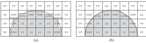
Finally, new configuration and distribution of fluid is known. The surface reconstruction method plays an important role in VOF method, which has a great effect on accuracy. A more accurate interface approximation leads to a smoother volume fraction distribution, hence a more precise calculation of surface normal is achieved. In earlier works, the simple line interface calculation (SLIC) method was generally used, which approximates the interface with a straight line aligned with one of the mesh coordinates. However, the SLIC method is a comparatively rougher approximation and is suitable in problems with less deformation involved. The piecewise linear interface calculation (PLIC) method which was
developed by Youngs,8) allows a non-zero slope for the
straight line to approximate the interface, and yields a more accurate interface approximation. These two methods are shown in Fig. 1, where Figs. 1(a) and (b) reconstruct different surface geometries from the same volume fraction data.
In this study, the PLIC method coupled with the VOF method were adopted to construct the interface and to calculate the transportation of fluid. The numerical scheme and procedures include the following three steps:
2.3.1 The construction/reconstruction of free surfaces
After the F-value of each cell is determined, the normal
vector of the interface can be calculated from the following equation:
~
n
n¼ rF ð4Þ
Therefore, the interface of a surface cell can be represented by the following equation for a plane:
xx~nn^¼0 ð5Þ
where xx~ is the position vector on interfaces, nn^ is the unit
normal vector of the plane, is a plane constant. The
negative sign indicates that the direction of the unit normal vector points into gas.
2.3.2 Solve for the velocity field
Velocity field and pressure field can be solved from (1) and (2). In this study, an explicit finite difference method and SOLA algorithm, which is a method for solving transient flow, were employed. According to SOLA scheme, a pressure adjustment term is derived from (1) and (2) as follows:
p¼ D
ð@D=@pÞ ð6Þ
In the beginning, a tentative velocity field at new time step is calculated from (1) with a prescribed pressure field at old time step. Then, the divergence is obtained from (2). If the divergence is not equal to zero, that means the calculated velocity and pressure fields could not satisfy the conservation
of mass, and the pressure adjustment termpis used to adjust
the tentative velocity field. The iteration process is continu-ing until zero divergence is satisfied for all the cells in the interior region.
2.3.3 Calculate the convection and redistribution ofF -values
After the velocity and pressure fields are calculated at new time step, the convectional fluid volume and the new location of free surface can therefore be computed in order to solve for
the redistribution ofF-values in each cell. The convectional
fluid volume in a layer is estimated approximately equal to the velocity of the cell multiplied by the time interval.
Therefore, three volume fluxes:ðþÞ
i;j;k,ðÞi;j;kandð0Þi;j;k
are calculated. ðþÞi;j;k and ðÞi;j;k represent the volume
fluxes flow from ði;j;kÞ cell to ðiþ1;j;kÞ and ði1;j;kÞ
cells respectively. ð0Þ
i;j;k is the remained fluid volume in
(a) (b)
0.943 1.0 0.943 1.0 1.0 1.0
1.0 1.0 1.0 1.0
0.0 0.0 0.0 0.0 0.0 0.0 0.0 0.0 0.0 0.0 0.0 0.0 0.0 0.0
0.029 0.029 0.576 0.943 0.943 0.576
0.576 0.576 0.943 0.943 1.0 0.0 0.0 0.029 0.029 0.576 0.943 0.943 0.576
0.576 0.576
0.0
0.0 0.0
0.0 0.0 0.0 0.0 0.0 0.0
0.0 0.0 0.0 1.0 1.0 1.0 1.0 1.0 1.0 1.0
[image:2.595.305.546.71.142.2]ði;j;kÞ cell. When the fluid flows out from ði;j;kÞ cell to
ðiþ1;j;kÞcell,ðþÞ
i;j;kis larger than zero andðÞiþ1;j;kis
equal to zero. When the fluid flows out from ði;j;kÞcell to
ði1;j;kÞcell,ðÞ
i;j;kis larger than zero andðþÞi1;j;kis
equal to zero. The three volume fluxes during one fractional step are regions under the convectional line, which shows in
Fig. 2. The redistributed volume fraction in each cell alongx,
y,zdirections is then can be given as follows respectively:
Fði;j;;xÞk ¼ ðþÞi1;j;kþ ð0Þi;j;kþ ðÞiþ1;j;k ð7Þ
Fði;j;;yÞk ¼ ðþÞi;j1;kþ ð0Þi;j;kþ ðÞi;jþ1;k ð8Þ
Fið;j;;zÞk ¼ ðþÞi;j;k1þ ð 0
Þi;j;kþ ð
Þi;j;kþ1 ð9Þ
where superscript means the F-value at new time step.
AfterF-value at new time step inx,y,zaxial coordinates are
computed from (7), (8) and (9), the redistribution ofF-values
can then be obtained.
2.4 Treatment of surface tension
In order to take the effect of surface tension into account, a surface-tension-induced pressure jump was used to represent a boundary condition in the pressure field at the interface in earlier studies. Therefore, the exact surface location and slope had to be computed in order to obtain the correct pressure at the free surface, and a reconstruction of a continuous surface was then required. In this study, a very different approach for reconstructing a continuous surface
developed by Brackbillet al.10)was adopted, which is called
the CSF model. In the CSF model, surface tension is interpreted as a continuous, three-dimensional effect across an interface, rather than as a boundary condition on the interface. Hence an interfacial surface force is replaced by a localized volume force acting on the interface, which can be added into the Navier–Stokes equations as a form of body force, and has effect on the velocity field.
In CSF model, the interface is regarded as a transition region where the fluid properties change continuously. When the thickness of the transition region is infinitesimal, the volume forceFF~b can be written as:
~
F
Fb¼nn^ ð10Þ
whereis the surface tension coefficient,nn^is calculated from
VOF data in (4),is the curvature of free surface, which can
be calculated from:
¼ ðr nn^Þ ð11Þ
This body forceFF~b acts everywhere in the transition region,
therefore the exact surface location is no longer required. This eliminates the need for interface reconstruction, and simplifies the calculation of surface tension.
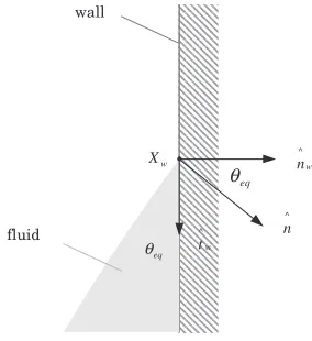
2.5 Treatment of wall adhesion
When molten solder contacts with the substrate, which includes the wettable solder pad and the nonwettable solder
mask, the fluid interface forms a contact anglewith the rigid
boundary. If the angleis equal to static contact angleeq, a
state of static equilibrium is reached. If not, a nonzero wall adhesion force results that trends to pull the fluid until
¼eq.11)This wall adhesion can be regarded as a volume
force due to surface tension at points of contact with ‘‘walls’’, therefore, it can be calculated in the same manner as (10), except that a boundary condition is applied to the free surface normal whose vertex lying on or near a rigid boundary. From Fig. 3, the wall adhesion boundary condition can be interpreted as the expression for the unit free surface normal
^ n
nat pointsxx~won the wall by geometric identity:
^ n
n¼nn^wcoseqþtt^wsineq ð12Þ
wherenn^wis the unit wall normal directed into the wall,tt^wis
tangent to the wall and normal to the contact line between the free surface and the wall atxx~w.
3. Experimental Method
The purpose of experiment conducted in this study is to validate the simulation result of the standoff height and maximum width of solder joints which are related to the change in solder volume. Therefore, solder volume has to be a known value. If the solder bump is made by electroplating, solder volume can not be known easily due to uneven electric current density. Thus, in this study, solder balls were melted together to reform new solder balls with different volume, which was the sum of original volume of each solder balls. The solder ball in use had three different sizes, which was
300, 500 and 760mm in diameter respectively, and its
composition was 63 mass Sn–37 mass Pb. After solder balls with different volume were made, they were then put onto solder pads with circular shape. These solder pads were
Cell boundaries Segment after advection
Segment before advection
(φ+)
i-1,j,k (φ0)i,j,k (φ-)i+1,j,k (i-1,j,k) (i,j,k)
ui-1/2,j,k ui+1/2,j,k (
i+1,j,k)
Fig. 2 Calculation of the volume fluxes during one fractional step.
eq
θ tw
^
^ n
eq
θ nw
^ w
X
wall
fluid
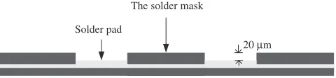
[image:3.595.354.496.72.227.2] [image:3.595.55.283.73.208.2]20mm lower than the solder mask, which can be seen in Fig. 4. The material of solder pads was Ni-Au, and the contact angle of molten solder formed on solder pad was
about 5 by measurement, while the molten solder made an
angle about 148.4on the epoxy material.
After the volume and contact angle on substrate of solder were known, solder balls put onto solder pads were sent into IR reflow furnace. After the reflow process, the standoff height and maximum width of solder joints were measured and were compared with simulation results.
4. Results and Discussions
4.1 The comparison with Surface Evolver in the simu-lation of contact angle
The change of contact angle of molten solder on substrate can both be simulated by Surface Evolver and the program developed in this study, and the simulation parameters in use
are shown in Table 1. Contact angle of 30, 50, and 75are
taken as examples for the comparison, which can be seen from Fig. 5. Figure 5 shows that there is a good coincidence in simulation results between Surface Evolver and the program developed in this study. In situation where the flow of molten solder on substrate is not restricted, the smaller the contact angle is, the larger the expansion area on substrate is. From the simulation result of the program
developed in this study in Fig. 5, the intensity of adhesive force can be measured by the surface normal of the first layer of molten solder in contact with the substrate. Thus, the smaller the contact angle is, the larger the normal vectors of interfaces are, which represent a greater adhesive force to the substrate.
4.2 The simulation of shape evolution of solder joints during reflow process
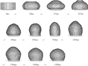
Since the program developed in this study is based on fluid dynamics, the flow behavior of molten solder during reflow process can be simulated by calculating the change of velocity field at each time step. However, Surface Evolver calculates the shape evolution of solder by conjugate gradient methods, which have no physical significance at every iteration step, especially when the volume of solder is too much to be constrained in the solder pad. Therefore, the understanding of the shape evolution of solder joints during reflow process has to depend on the simulation based on fluid dynamics scheme, such as the program developed in this study. The simulation results are shown in Fig. 6, and the
solder volume is set to be 0.2298 mm3.
As can be seen from Fig. 6, if the initial shape of solder is a cylinder, it evolves into sphere gradually with time during reflow process due to the effect of surface tension. In the program developed in this study, the solder mask can be set to be higher than solder pad as the actual situation, which is not achievable by Surface Evolver. Thus the simulation results can be closer to the real situation when the solder mask has great influence on the flow of molten solder. However, it is impossible to take the pictures of molten solder during reflow
process in106second such a short interval, especially when
the temperature in reflow furnace is over 220C. Therefore,
this simulation result can not easily be validated with experiment.
4.3 The effect of solder volume with experimental validation
Considering the effect of solder volume, solder balls of different volume were put onto circular solder pads which
are 600mmin diameter. The standoff height and maximum
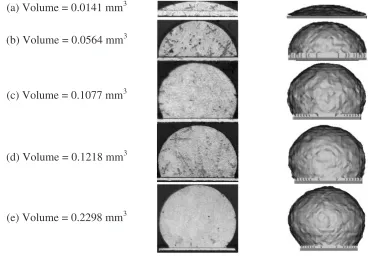
[image:4.595.50.290.74.130.2]width of solder joints after reflow, was measured and then compared with simulation results. It can be seen from Fig. 7, that simulation results consist with the experimental measurements very well. Therefore, the accuracy of the program developed in this study is verified in an accurate range. On the solder pad of the same size, the standoff height and maximum width of solder joints increase with increasing solder volume. However, simulation results are slightly larger than the experiment measurements, and this may due to the volume shrinkage during the solidification of solder.
The shape of solder joints are observed from the cross sections, which are compared with simulation results as shown in Fig. 8. As can be seen from Fig. 8, the contact angle formed in solder pads increases with the increasing solder volume. It is different from situation in Fig. 5, where the expansion of solder on the substrate is not restricted, and contact angle of solder is irrelevant to the solder volume. In Figure 8, the flow of solder is confined in solder pads by the
Solder pad
The solder mask
20 µm
[image:4.595.46.291.537.753.2]Fig. 4 The cross section of BGA substrate.
Table 1 The simulation parameters used in this study.
(a) In the program developed in this study
Composition of solder Density Viscosity12Þ Surface Tension12Þ
63%Sn–37%Pb 8.9 g/cm3 0.002237 Pas 49.853 N/m
(b) In Surface Evolver
Composition of solder Density Surface Tension
63%Sn–37%Pb 8.9 g/cm3 49.853 N/m
Surface Evolver Program developed in this study
(a) Contact angle of 30°
(b) Contact angle of 50°
(c) Contact angle of 75°
[image:4.595.45.291.538.612.2] [image:4.595.44.291.547.748.2]nonwettable solder mask, which is 20mmhigher than solder pads. Therefore, the contact angle of solder is different from the static contact angle value, and is proportional to the solder volume.
4.4 The effect of size and shape of solder pad
Solder volume of 0.0141 mm3 were put onto circular
solder pads which were 600 and 420mm in diameter
respectively. The simulated standoff height and maximum width of solder joints after reflow are listed in Table 2. From Table 2 it can be seen that the solder joint on the solder pad with larger size has the lower standoff height, which due to the larger wettable area.
If the size of solder pad is fixed, the effect of the shape of solder pad is able to be observed. The solder pad area of
0.2827 mm2 was used. Then solder volume of 0.2298 mm3
was put onto the circular and rectangular solder pads respectively. The simulated tandoff height and maximum width of solder after reflow are shown in Table 3. As can be seen from Table 3, there is no much difference in standoff height and maximum width of solder between on circular and rectangular solder pad, except for slightly lower in height and smaller in width of solder on the circular solder pad.
Therefore, the shape of solder joints is observed in Fig. 9. It shows that on circular and rectangular solder pads of equivalent area, the length of rectangular solder pad is slightly larger than the diameter of circular solder pad. Moreover, the distribution of molten solder on the circular solder pad is more uniform than on the rectangular solder pad but not disperse into four corners as on the rectangular pad. This may causes slightly lower in height and smaller in the width of solder joint on the circular solder pad.
0µs 69µs 151µs 227µs
446µs 681µs 944µs 1265µs
1366µs 1440µs 1508µs
Fig. 6 The simulation of shape evolution of solder joints during reflow process.
0.00 0.05 0.10 0.15 0.20 0.25
0 100 200 300 400 500 600 700 800 900 1000
Experiment Simulation
Volume (mm
Standoff Height (
µ
m)
Maximum Width (
µ
m)
3 )
0.00 0.05 0.10 0.15 0.20 0.25
0 100 200 300 400 500 600 700 800 900 1000
Experiment Simulation
Volume (mm3)
(a) The change in standoff height
(b) The change in maximum width
[image:5.595.109.484.81.362.2] [image:5.595.111.488.404.558.2]4.5 The effect of wettability of the solder mask
The contact angle of molten solder on substrate was used to characterize the wettability of substrate in this study.
Contact angle of 90and 148were used to represent solder
masks of two materials, where contact angle of 90 had
inferior wettability to molten solder. Solder volume of
0.2298 mm3 was put onto the circular solder pad which was
600mm in diameter, and the solder masks of different
wettabilities were compared as shown in Fig. 10. In the same solder volume, when the wettability of the solder mask is inferior, the ability of the solder mask to confine the molten
solder in the solder pad is better. Contact angle of 90of the
solder mask shown in Fig. 10 apparently can not constrain such mass of solder in the solder pad, and causes the solder
flow out onto the solder mask, thus a contact angle of 90
between the solder and the solder mask is formed. Therefore, when the volume of solder is larger, an overflow condition is appeared if the restriction of the solder mask is not enough. In the simulation by Surface Evolver, the wettability of the solder mask is not considered since the molten solder is assumed not flow out onto the solder mask.
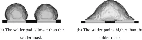
4.6 The effect of the position of the solder mask
In the same bump pitch, the volume of solder should be larger enough to allow for the assembly, but not too large to cause the contact of adjacent solder joints and make the short in circuit. Therefore, a maximum volume of solder under the given bump pitch is imperative to obtain. In this study, the position of the solder mask was considered to understand its effect on the determination of maximum volume of the solder, which was not able to be considered in Surface
(a) Volume = 0.0141 mm
3(b) Volume = 0.0564 mm
3(c) Volume = 0.1077 mm
3(d) Volume = 0.1218 mm
3(e) Volume = 0.2298 mm
3 [image:6.595.111.480.74.330.2]Fig. 8 The experimental observation on cross sections of solder joints of different volume compared with simulation results.
Table 2 The effect of size of solder pads on solder joints.
Diameter of solder pad
Standoff height of solder
Maximum width of solder
600mm 80mm 591.9mm
420mm 175mm 454.1mm
[image:6.595.307.545.373.458.2]Solder volume = 0.0141 mm3
Table 3 The effect of shape of solder pads on solder joints.
The shape of solder pad
Standoff height of solder
Maximum width of solder
Circular 650mm 812.6mm
Rectangular 626.6mm 823.8mm
Solder volume = 0.2298 mm3, solder pad area = 0.2827 mm2
(a) Solder joint on circular solder pad (b) Solder joint on rectangular solder pad
Fig. 9 The comparison of the simulation results in shape between solder joint on circular solder pad and on rectangular solder pad.
(a) The contact angle of the solder mask
is 148°.
(b) The contact angle of the solder
mask is 90°.
[image:6.595.47.290.381.434.2] [image:6.595.46.291.483.536.2] [image:6.595.56.279.576.630.2]Evolver. Two cases were compared: the solder pad is lower than the solder mask, and the solder pad is higher than the solder mask. A given volume of solder is the same, one can be seen in Fig. 11, that adjacent solder joints contact with each other in the situation where the solder pad is higher than the solder mask. Thus, under the restriction of the thickness of solder mask, the larger maximum volume of solder is obtained in the same bump pitch.
5. Conclusions
In order to understand the shape evolution of solder joints during reflow process, a three-dimensional computer-aided analysis system based on fluid dynamics has been developed in this study. The developed program is capable of simulating the change of contact angle of the solder on the substrate, which is consistent with the simulation results by the energy-based algorithm, the Surface Evolver. In addition, the effect of solder volume on the shape of solder joints was simulated and the results were verified to have good coincidence with experimental measurements. Furthermore, the effect of size and the shape of solder pad were simulated and reasonable results were obtained.
On the advantage of using algorithms based on fluid
dynamics, the shape evolution of solder joints during reflow process and the overflow condition of the molten solder were able to simulate. Moreover, the physical properties of the solder mask such as wettability and thickness were allowed to consider, which was not achievable by the Surface Evolver.
Acknowledgements
This work has been supported by the National Science Council in Taiwan (NSC92-2216-E-006-041), for which the authors are grateful.
REFERENCES
1) H. K. Charles and G. V. Clatterbaugh: ASME Journal of Electronic Packaging112(1990) 135–146.
2) M. K. Shah: ASME Journal of Electronic Packaging118(1990) 122– 126.
3) K. N. Chiang and C. A. Yuan: IEEE Transactions on Advanced Packaging24(2001) 158–162.
4) K. A. Brakke: Version 2.20, Mathematics Department, Susquehanna University, Selinsgrove, 2003.
5) K. A. Brakke: Experimental Mathematics1(1992) 141–165. 6) C. W. Hirt, B. D. Nichols and R. S. Hotchkiss: Technology Report
LA-8355, (Los Alamos Scientific Laboratory, 1980).
7) C. W. Hirt and B. D. Nichols: J. Comput. Phys.39(1981) 201–225. 8) D. L. Youngs:Numerical Methods for Fluid Dynamics, ed. by K. W.
Morton and M. J. Baines, (Academic Press, 1982) pp. 273–285. 9) A. Celic and G. G. Zilliac:Computational Study of Surface Tension and
Wall Adhesion Effects on an Oil Film Flow Underneath an Air Boundary Layer, (NASA Ames Research Center, USA, August 1997). 10) J. U. Brackbill, D. B. Kothe and C. Zemach: J. Comput. Phys.100
(1992) 335–354.
11) D. B. Kothe, R. C. Mjolsness and M. D. Torrey: ‘‘RIPPLE: A Computer Program for Incompressible Flows with Free Surfaces’’, LA-12007-MS, April 1994.
12) M. Dietzal, S. Haferl, Y. Ventikos and D. Poulikakos: J. Heat Trans. 125(2003) 365–376.
(a) The solder pad is lower than the
solder mask
(b) The solder pad is higher than the
[image:7.595.50.287.74.142.2]solder mask