Munich Personal RePEc Archive
Stagnation and minimum wage: Optimal
minimum wage policy in macroeconomics
Yamaguchi, Masao
Osaka University of Economics
3 August 2017
Online at
https://mpra.ub.uni-muenchen.de/80359/
Stagnation and minimum wage: Optimal minimum wage
policy in macroeconomics
Masao Yamaguchi∗
August, 2017
abstract
This paper argues how an increase in minimum wage affects employment, con-sumption, and social welfare with dynamic general equilibrium model without mar-ket frictions. The study demonstrates that a minimum wage hike reduces an ac-tual unemployment rate and has positive effects on an employment rate under the demand-shortage economy whereas they do not under a non-demand shortage econ-omy. The study also shows that optimal minimum wage which maximize social welfare and minimize an actual unemployment rate when the economy faces the demand-shortage initially. These findings imply that the minimum wage can be considered as one of the effective policy for overcoming deflation and stagnation although it increases the natural rate of unemployment.
KEYWORDS: Minimum wage, Unemployment, Natural rate of unemployment,
De-flation, Stagnation, Demand shortage, Dynamic general equilibrium model
JEL Classification Codes: E24 E31 J38
1
Introduction
The model of the competitive labor market states that a decline in minimum wage
(above competitive wage) increases the employment, firm’s profits, and welfare and
thus vitalizes the economy. During the depression period, however, this effects do not
seem to work well because a decrease in aggregate demand is a significant factor that
decline an employment rate as Keynes (1936) explained. What does macro-economy
∗Corresponding author: Faculty of Economics, Osaka University of Economics, 2-2-8, Osumi,
respond when the government increases minimum wage in the stagnation? This paper
argues that the impact of minimum wage policy on the economy differs in response to
the economic situation, and shows that when an economy faces a demand shortage,
an increase in minimum wages improves the employment rate, aggregate consumption,
and social welfare. On the other hand, in an economy that does not face demand
shortage, the increase in wages worsens the employment rate, aggregate consumption,
and social welfare. Trade unions often insist on wage hikes during the labor-management
negotiations, arguing that wage hikes will stimulate the consumption and aggregate
demand. This paper supports these opinions in the context of an sluggish economy but
not of an booming economy.
I develop a simple extension of Ono’s (2001) dynamic general equilibrium model
with-out market frictions by building in two different types of jobs. In the model economy,
single final goods are produced by two labor inputs. Firms pay an efficiency wage and
a minimum wage for each job. This assumption gives rise to a positive link between
efficiency wage and minimum wages that can be used to analyze the effect of a wage
hike (caused by a minimum wage hike) on the economy. This wage setting enables a
tractable analysis because the minimum wage hike leaves the relative wage of each job
unchanged, which eliminates the effect of substitution of labor demand for each job.1
Therefore, the model can focus on the other effects of the minimum wage hike such as
on inflation and the budget constraint of households that is unnoticed earlier.
Households have utility from consumption and real balances of money. Assumption
of insatiable marginal utility of money generates two different equilibria: a
demand-shortage and a supply-side (non-demand-demand-shortage) economy as Ono (2001) showed. If
the marginal utility of money is insatiable, the households accumulate money more than
enough, and hence, the aggregate consumption level falls short of aggregate output level,
that is, the demand-shortage equilibrium comes out. If the marginal utility of money is
satiable, the supply-side equilibrium shows up. In the analysis, contrasting a
demand-shortage and supply-side economy sheds new light on the function of a minimum wage.
In a demand-shortage economy, the minimum wage hike can prominently increase
ag-gregate consumption, decrease an actual unemployment rate, and improve social welfare.
The reason for this result is attributable primarily to a firm’s labor demand function.
When the firm faces the demand-shortage constraint, an equilibrium of
underemploy-ment arises in which the marginal product of labor is higher than the wage. Hence,
higher aggregate demand induces the firms to increase their labor demand and to
de-crease the underemployment as Barro and Grossman (1971) and Honkapohja (1980)
1Cahuc and Michel (1996) state that the minimum wage hike increases the relative wage of unskilled
showed.2 At the same time, an increase in the minimum wage narrows the
disequilib-rium gap between demand and supply caused by the stimulation of consumption and
then eases deflation. In other words, there is an optimal minimum wage policy that
maximizes social welfare and minimizes an actual unemployment rate when the
econ-omy faces the demand-shortage initially. The analysis also provides a policy implication
for governments concerned about budget deficit–that is, a minimum wage hike can raise
the aggregate demand without an increase in government spending.3
On the other hand, in a supply-side (non-demand-shortage economy), a minimum
wage hike decreases the employment and worsens the social welfare in analogy with the
competitive labor market model.
A number of studies are related to this work. As stated above, I use the setting of
Ono’s (2001) dynamic general equilibrium model with perfect information. Ono shows
the reasons for the occurrence of liquidity trap and a stagnation, but he does not discuss
the impact of minimum wage.
The minimum wage policy is controversial although its empirical results of
employ-ment effects seem elusive (Manning 2016). Lots of empirical studies analyze the
min-imum wage effects on the employment.4 Several theoretical studies argue the positive
function of minimum wage as opposed to the standard model. The welfare-enhancing
minimum wage policy can be obtained by the intensifying capital accumulation. Cahuc
and Michel (1996) and Fanti and Gori (2011) consider a growth model in which minimum
wage hikes can improve welfare, but for reasons that are different from those we consider
here.5 In their model, a minimum wage hike increases savings and capital accumulation
at the cost of increasing unemployment. It then improves economic growth and welfare
under generous unemployment benefits and the positive externality of human capital
accumulation that stem from the substituting skilled labor for binding minimum-wage
low-skilled labor. In a context of search model Flinn (2006) shows that minimum wage
2Honkapohja (1980) considers disequilibrium model with endogenous money holdings of household
and shows that the steady state effect of an increase in real government expenditure with the case of endogenous money holdings is larger than the fixed price case with exogenous money holdings.
3Annual inflation rate in the euro zone and in Japan are 0.2%and -0.1%in 2016, respectively. It
is also worth considering the minimum wage policy to stimulate the economic activity and to alleviate the diminishing price pressures.
4For instance, regarding the minimum wage policy effect on low wage employment, Neumark, Salas
and Wascher (2014) conducts a controversy with Allegretto, Dube, and Reich (2011), and Dube, Lester, and Reich (2010). Further Allegretto, Dube, Reich, and Zipperer (2017) offer a counterargument against Neumark et al. (2014).
5Some studies focus on the relation economic growth and minimum wage. Irmen and Wigger (2006)
improves unemployment inefficiency and may increase employment considering the size
of the searching participants in response to the minimum wage.6 Furthermore, in the
monopsony model as is well known, a minimum wage hike can increase the employment
and improve the welfare.7 Moreover, Lee and Saez (2012) show the minimum wage hike
becomes the social optimal under competitive labor markets with labor market
hetero-geneity when social welfare function is assumed to value redistribution from high wage
to low wage workers.8 However, none of these studies focus on the optimal minimum
wage policy implemented under demand shortage.
The rest of the paper is organized as follows. Section 2 explains the basic setting of
the model. The effects of a minimum wage are analyzed in a supply-side economy in
section 3 and in a demand-shortage economy in section 4. Section 5 discuss the optimal
minimum wage policy. Section 6 concludes the paper.
2
The model
2.1 Firms
Consider an economy without market frictions in which a representative firm produce
final goods. Two labor are used in production. One is ”high-wage job” which is
char-acterized that workers’ effort increase output, and hence the firm pays the efficiency
wage for this labor. The other is ”low-wage job” characterized that workers’ effort is
not response to the output, and hence the firm pays a minimum wage for this labor. I
assume that the minimum wage is regulated and its level is greater than the competitive
wage.9
The concave production function is given by
y= (en1)anb2, 0< a, b <1, (1)
wherey denotes the amounts of output produced andn1 andn2 stand for the number of
employees of high-wage and low-wage job, respectively. eindicates productivity affected
6Acemoglu (2001) constructs a search model in which high and low-wage jobs coexist in response to
capital intensity of each industry and demonstrates that introducing a minimum wage shifts the com-position of employment toward high-wage jobs, increases average labor productivity, and may improve welfare.
7Manning (2003) discusses the monopsony in greater detail. Bhaskar and To (1999) construct the
monopsonistic competition, where a large number of employers compete for workers, and are able to freely enter or exit. A rise in minimum wage raises employment per firm but causes firm’s exit due to the decline of their profit. If the labor market is sufficiently distorted, the rise in minimum wage raises aggregate employment and welfare.
8With labor market heterogeneity, Revitzer and Taylor (1995) build on the sharking model of Shapiro
and Stiglitz (1984) and show that the increase in minimum wage may raise the employment rate.
9I assume that the low-wage job worker does not shirk, because the firm utilizes monitoring technology
by the worker’s effort, and its functional form is
e=
(w
1−x
x )θ
, 0< θ <1, (2)
wherew1is a real wage andxis reference point that equals a reservation wage (See below
in detail). Equation (2) shows that an increase in wage margin from the reservation wage
raises productivity. The firm chooses the level of real wage that minimize cost per unit
of the effective labor input, w1/e, which is modeled by Summers (1988). The optimal
real wage and effort level are
¯
w1 =
x
1−θ, (3)
¯
e=
( θ
1−θ )θ
. (4)
The firm is a price taker and sells the final goods at a price P competitively. When
they can sell all the output under the exisiting levels of wages and price, employment are
determined so that marginal products of each labor equal to their costs. The optimal
conditions are
¯
ea(¯en1)a
−1
nb2 =w1, (5)
b(¯en1)anb2−1 =w2, (6)
wherew2is a real wage of low-wage workers. I refer to this economy as supply-side
(non-demand-shortage) regime because the output and employment level are determined by
not demand-side factors but supply-side factors.
On the other hand, when the firm is not be able to sell its notional output under
the exisiting levels of wages and price, the firm chooses optimal employment subject to
aggregate demand constraint as follows.
max n1,n2 y
−w1n1−w2n2
whereyd is aggregate demand. The optimal conditions are10
(¯en1)anb2 =yd, (7)
an2
bn1
= w1
w2
. (8)
In (7) and (8), the marginal products of each labor is higher than its cost because
firm faces the limiting aggregate demand. This setting is formulated by Barro and
Grossman (1971). I refer to this economy as demand-shortage regime. The employment
level detemined by the firm under demand shortage regime is smaller than that under
supply-side regime.
2.2 Wage determination and employment
The firm’s setting of efficiency wage depends on the reservation wage x as in (3),
which equals to the worker’s expectation wage when he/she loses the present job.11
x=n1w1+n2w2. (9)
Substituting (9) into (3) yields
w1 =
n2w2
1−θ−n1
. (10)
I assume θ <1−n1 to assure the existence of a solution. Equation (10) predicts that
the circumstances of the labor market affect the wage of high-wage job workers. The
increase inw2,n1, andn2 raise the reservation wage and the wage of the high-wage job
workers.
Using (10), (5) and (6), the equilibrium employment for each type of labor in the
supply-side regime economy become
n1=
a(1−θ)
a+b ≡n
s∗
1 , (11)
10As is shown by Ono (2001), the demand shortage arises not due to price rigidity but due to
house-holds’ preference. The firm knows that the demand shortage cannot be eliminated in spite of price adjustments. Thereby the firm maxmizes their profits given the constraint of demand shortage. The optimal condition of the problem can be written by the Lagrangian multiplier method as follows:
max
n1,n2,κ L= (¯en1) a
nb2−w1n1−w2n2+κ((¯en1)anb2−y
d
)
The optimal conditions are
(1 +κ)¯ea(¯en1)a−1nb2=w1,
(1 +κ)b(¯en1)anb2−1=w2,
(¯en1)anb2−yd= 0.
11Falk, Kehr, and Zehnder (2006) show minimum wages have significant effects on reservation wages
n2=
( b w2
)11
−b(ea¯ (1−θ) a+b
)1−ab
≡ns∗
2 (w2),
dns∗
2
dw2
=ns∗
2
′
(w2)<0. (12)
The increase in minimum wage reduces the employment ns∗
2 but does not affect the
employment ns∗
1 .12 This implies that the employment is determined by only the labor
market variable. Substituting equilibrium employment level (11) and (12) into
produc-tion funcproduc-tion (1) gives aggregate output level:
y= (¯ens∗
1 )a(ns
∗
2 (w2))b ≡ys∗(w2),
dys∗
dw2
<0. (13)
On the contrary, aggregate demand affects the employment Under demand shortage.
This relation is derived from (10), (7) and (8) as follows.
n1 = a(1
−θ)
a+b , (14)
n2 =
( yd)
1
b (ea¯ (1−θ) a+b
)−ab
. (15)
2.3 Households
Infinitely lived households have a utility function of the form
U =
∫ ∞
0 e
−ρt[u(c) +v(m)]dt, (16)
whereρis a constant rate of time preference, andu(c) andv(m) are a continuous concave
instantaneous utilities of real consumption c and real money balances m, respectively.
I abbreviate the time notation of each variable to simplify exposition. The households
provide one unit of labor inelastically. Population size in a economy is equal to 1. The
households are ex ante identical, and the allocation of their labor to high-wage or
low-wage jobs is done through a lottery. The households are then divided into two types
by their employment status, with each type having different budget constraints. One
engages in the high-wage job that receives the efficiency wagew1, and the other engages
in the low-wage job that receives the minimum wagew2.
Each household chooses the optimal consumption and the real money balances to
maximizeU, subject to the following flow budget constraint:
˙
m1=w1+
q n1
−z1−c1−πm1, (i= 1), (17)
12This is because the model assumes the Cobb-Dougulas production function. ∂ns∗
1
∂w2 > 0 when f22n2
f2 − f12n2
f1 + 1 > 0 with concave non-homothetic production function f(n1, n2(w2)) or elasticity
of substitution is more than 1 with CES production function, where fj ≡ ∂f(∂nn1,n2)
j , (j = 1,2) and
fjk=
∂fj(n1,n2)
∂nk , (k= 1,2). I do not consider this case because this paper focuses on the other effects
˙
m2=w2−z2−c2−πm2, (i= 2). (18)
Variables such asc,m,n,w, and , z are denoted by suffixi= 1 if he/she has the
high-wage job, andi= 2 for the low-wage job.13 zi(≥0) is a lump-sum tax. I assume that a
firm’s real profit,q ≡(¯en1)anb2−w1n1−w2n2, is equally distributed to the households of
high-wage job.14 π is a inflation rate. Then, the first-order conditions of each household
are
ηci
˙
ci
ci
= v
′
(mi)
u′(c
i)
−ρ−π, (i= 1,2), (19)
whereηci ≡
−u′′(c
i)ci
u′(ci) >0. The transversality conditions are
lim
t→∞λi(t)mi(t)e
−ρt = 0, (i= 1,2), (20)
whereλi(t) is a costate variable of mi.
At any point in time, the money market is in equilibrium.
ms=n1m1+n2m2, (21)
where ms indicates the real money stock. The percentage change in the money stock
depends on the government’s money expansion rate, µ≡ MM˙ss, and the inflation rate,π.
˙
ms
ms =µ−π. (22)
Gorvernment spending g is financed by monetary expansion and households’ taxation.
Therefore, the government’s budget constraint is
g=msµ+n1z1+n2z2, (23)
wheremsµ= Ms
P
˙
Ms
Ms.
The aggregate demand consists of the consumption of households and the gorvernment
spending.
yd=c1n1+c2n2+g. (24)
In the same manner as Ono(2001), the rate of change of prices depends on gap between
13The behavior of unemployed people is not considered in the model. That is, the model assumes
implicitly that unemployed people are parasites on their friends or relations who have a job.
14This assumption is for the simplicity. Meanwhile, it is possible to build in the stock market, in
aggregate supply and demand.
π =α [
yd
ys∗(w
2)
−1
]
, α >0, (25)
where π denotes the inflation rate and α stands for the adjustment speed of the price.
Excess demand (supply) pushes up (down) the inflation rate.
2.4 Equilibria
The system of consolidated equations is shown as follows.
˙
c1 =
c1
ηc1
[ v′
(m1)
u′(c
1)
−ρ−α (
yd
ys∗(w
2)
−1
)]
, (26)
˙
c2 =
c2
ηc2
[ v′
(m2)
u′(c
2)
−ρ−α (
yd
ys∗(w
2)
−1
)]
, (27)
˙
m1=
(¯en1)a(n2)b−w2n2
n1
−z1−c1−α
( yd
ys∗(w
2)
−1
)
m1, (28)
˙
m2=w2−z2−c2−α
( yd
ys∗(w
2)
−1
)
m2, (29)
yd=c1n1+c2n2+g, (30)
where (30) is derived from equation (23) in which I assume µ = 0. Equations
(26)-(29) form an autonomous dynamic system with respect to c1, c2, m1 and m2 under the
equation (30), exogeneous minimum wage w2, the output level ys∗(w2) in (13), and
the predetermined variables n1 and n2 which are determined in (11) and (12) under
non-demand shortage meanwhile in (14) and (15) under demand shortage.
To show the effect of minimum wage on economy clearly, I focus two steady state
equilibria such that
˙
c1 = 0, c˙2 = 0, m˙1 = 0, m˙2 = 0, π= 0, (31)
which is called supply-side regime equilibrium and,
˙
c1= 0, c˙2= 0, m˙1=−
msπ
n1
, m˙2= 0, π <0, (32)
which is called demand-shortage regime equilibrium. The steady state in (32) entails
persisting deflation π <0 by supposing an addition assumption as explained below.
In the next section the supply-side regime equilibrium is analyzed, and after that, the
3
Minimum wage effects in supply-side regime equilibrium
The system (26)-(30) reaches to a steady state equilibrium as represented in (31)
when the stability conditions (Assumption 1 in Appendix) are satisfied. This is shown in
Appendix. In this steady state, consumption and real money balances of each household
become constant, the gap between aggregate supply and demand is plugged, that is,
π= 0, and the employment rate of each job is determined by (11) and (12). The steady
state equilibrium values are obtained (see Appendix A.2) as follows:
cs∗
i =csi(w2),
dcs∗
1
dw2
<0, dc
s∗
2
dw2
=sign(1 +ms∗
1 πcs1+m
s∗
2 πcs1
ns∗
2
ns∗
1
−ms∗
2 πsw2), (33)
ms∗
i =msi(w2),
dms∗
1
dw2
<0, dm
s∗
2
dw2
=sign(1 +ms∗
1 πcs1+m
s∗
2 πcs1
ns∗
2
ns∗
1
−ms∗
2 πws2), (34)
where the superscripts∗
indicates the equilibrium value. The increase in the minimum
wage entails an overall wage rise, and which affects consumption and money holdings
through each household’s budget and the inflation rate. In the steady state equilibrium,
the increase in the minimum wage reduces the consumption and money balances of
high-wage job householdscs∗
1 and ms
∗
1 , because it is mainly affected by the decreases in
real income which consists of their wages and distributed income from profit.15
But it may raise thecs∗
2 , ms
∗
2 when the effect ofπws2 in (33) and (34) is small enough
because it is affected by the increase in real income which is just caused by the minimum
wage hike. On the whole, the minimum wage hike lowers the aggregate consumption
level, that is, d(cs1∗n1s∗+cs2∗ns2∗)
dw2 < 0, which entails a decrease in aggregate output level,
because the negative effects of cs∗
1 and ns
∗
2 dominates the effects of cs
∗
2 . This result is
summed up as follows.
Proposition 1 In supply-side regime equilibrium, a minimum wage hike reduces the total consumption and aggregate output level.
Further, unemployment rate in the supply-side regime equilibrium can be expressed
asus∗
= 1−ns∗
1 −ns
∗
2 (w2) where dn
s∗
2 (w2)
dw2 <0 andn
s∗
1 is determined by deep parameters.
Therefore the minimum wage hike leads to the increase in unemployment rate. This is
shown as in Proposition 2:16
Proposition 2 In supply side regime equilibrium, a minimum wage hike raises an un-employment rate.
15The real income of household 1 isw
1+nq11 = y∗s(ws∗
2 )−w2ns2∗
ns∗
1
.
16∂us∗
∂w2 > 0 when f22n2
f2 − f12n2
f1 + 1 + f11n1
f1 − f21n1
f2 − n1
1−θ−n1 >0 with a concave non-homothetic
production function or elasticity of substitutionσwith CES production function satisfies 2
σ >1− n1
Moreover, social welfareVs can be expressed as
Vs=
∫ ∞
0
ns∗
1 (u(cs
∗
1 ) +v(ms
∗
1 ))e
−ρtdt+∫ ∞
0
ns∗
2 (u(cs
∗
2 ) +v(ms
∗
2 ))e
−ρtdt
= 1
ρ[n
s∗
1 (u(cs
∗
1 ) +v(ms
∗
1 )) +ns
∗
2 (u(cs
∗
2 ) +v(ms
∗
2 ))]. (35)
Differentiating (35) with minimum wagew2 throughcsi∗, ms
∗
i ,(i= 1,2), ns
∗
2 , Proposition
3 is obtained (see Appendix).
Proposition 3 In supply-side regime equilibrium, a minimum wage hike reduces the social welfare if
ε > dcs−∗1
1
dw2n
s∗
1
[(dcs∗
1
dw2
ns∗
1 +
dcs∗
2
dw2
ns∗
2
) ( u′
(cs∗
2 ) +ρ
u′′
(cs∗
2 )
v′′(ms∗
2 )
)
+dn
s∗
2
dw2
(u(cs∗
2 ) +v(ms
∗
2 ))
] .
Whereεindicates a subtractionu′
(cs∗
2 ) +ρ
u′′(cs∗
2 )
v′′(ms∗
2 ) from u
′
(cs∗
1 ) +ρ
u′′(cs∗
1 )
v′′(ms∗
1 ). Ifεis higher
than a certain negative value as in Proposition 3, the ambiguous effects of minimum
wage hike on consumption cs∗
2 in (33) and money balances ms
∗
2 in (34) become lower
than the total decreasing effects on cs∗
1 and ms
∗
1 , and then the minimum wage hike
reduces the social welfare. For example when ε= 0, the social welfare deteriorates by
the minimum wage hike.
4
Minimum wage effects in demand-shortage regime
equi-librium
Demand shortage regime equilibrium with deflation represented in (32) can be
gener-ated by supposing an additional assumption of money utility. In the supply-side regime
economy, I assume implicitly that the marginal utility of money converges to zero as the
households increase their real money balances, that is, limmi→∞v
′
(mi) = 0, (i= 1,2).
Here, the marginal utility of money of high-wage households is assumed to be insatiable
which is assumed by Ono (2001). This assumption emphasize a role of money holding
which generate not only transaction motive but also social power, status and prestages.17
Assumption of marginal utility of money
lim m1→∞v
′
(m1) =β >0, (36)
17Ono, Ogawa and Yoshida (2004) show empirically that the marginal rate of substitution of
The lower boundβ of marginal utility is coming up as the high-wage job households
increase money holdings. This assumption transforms the Euler equation (26) into
ηc1
˙
c1
c1
=
v′(m1)
u′(c1) −ρ−π, m1 is not big enough, β
u′(c1)−ρ−π, m1 is big enough.
(37)
When money holding increases marginally, the present consumption increases in
re-sponse to the decreasing marginal utility of money in the steady state equilibrium of
the first equation of (37), but the present consumption does not respond in the second
equation of (37). This invokes a demand shortage and deflation, even if the price adjusts
a disequilibrium of demand and supply in the goods market as in (25).
From (15), (27)-(30), and (37), the steady state equilibrium in (32) can be expressed
as consolidated two equations.
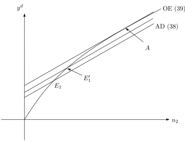
yd=c1(yd, w2)n1+c2(yd, w2)n2+g, (38)
n2 =
( yd)
1
b
(ea¯ (1−θ) a+b
)−ab
, (39)
where Appendix shows the saddle stability conditions of this equilibrium and explains
the derivation of (38). (38) indicates the aggregate demand in response to
employ-ment n2 which is depicted as a upward-sloping line AD in Fig.1. (39) represents the
relationship between aggregate output level and employment n2, i.e., the employment
determination equation through the production function when firms face the demand
shortage. This diagram is similar to the so-called Keynesian cross implying aggregate
demand determines aggregate output. E1 is demand shortage regime equilibrium given
a constant minimum wagew2.
As minimum wage increases, the AD line moves to upper direction and the steady
state equilibrium shifts fromE1toE1′. This increases the equilibrium aggregate demand
ydand employmentn
2 and thus the unemployment rate falls down. At this moment the
deflation becomes milder by reaction of the shrinking gap between aggregate demand
ydand potential aggregate outputy∗s(w
2) which is caused by the increase inydand the
decrease in y∗s(w
2). In this process, the rising inflation rates raises the consumption
c1 in (37). At the same time, the minimum wage hike also raises a real income of
household 2 and their consumption. In respose to the increase in the total consumption
and aggregate demand, the firm increases the employment.18 These results are summed
18In the initial steady state before the government raises the minimum wage. The government set the
n2
yd
AD (38) OE (39)
E1
E′
1
[image:14.595.169.483.65.306.2]A
Fig 1: Determination of employment and aggregate demand
up in Proposition 4 and 5.
Proposition 4 In demand-shortage regime equilibrium, a minimum wage hike raises aggregate demand, total consumption and employment, and also alleviates
defla-tion.
Proposition 5 In demand-shortage regime equilibrium, a minimum wage hike decreases unemployment rates.
Incidentally in pointA, the aggregate demandADbecomes tangential to the
produc-tion funcproduc-tion OE in which the point that the aggregate demand yd equals aggregate
outputys(w
2). To prove this fact, in equilibriumA, it require to show that the slope of
aggregate demand AD is just wA
2 refered to the minimum wage in equilibrium A. The
budget constraint in (29) becomes c2 =wA2 −z2 under inflation rate π = 0 and then,
the AD equation (38) is yd= (c1+z1)n1+wA2n2. The slope of this line becomes just
w2. dy
d
dn2 =w
A
2.19
On the other hand, in the steady state equilibrium of supply side regime, the
employ-ment rate ns∗
2 (wA2) is determined by (12) and the marginal productivity of n2 equals
towA
2. This implies that in pointA the production function has the tangent line that
slopes equals to wA
2. Thus the employment leveln2 under demand shortage inA is just
wage in proportion to the inflation rate that is higher than initial steady state. Note that in the new steady state equilibrium, the inflation rate becomes higher.
19Substitutingc
2=w2−z2 into aggregate demand yieldsyd= (c1+z1)n1+w2n2, wherec1in point
equals to ns∗
2 (w2A), and then the aggregate demand yd equals to the aggregate output
y∗s(wA
2).
Proposition 6 When minimum wage have increased and the equilibrium has reached to point A, the supply and demand gap has disappeared and then inflation rate π
has become zero. In this point the demand shortage regimes alters to supply side
regime.
In analogy with (35), social welfare in the demand-shortage regime equilibrium Vd
can be expressed as
Vd= 1
ρ [
nd∗
1 u(cd
∗
1 ) +nd
∗
2 u(cd
∗
2 ) +nd
∗
2 v(md
∗
2 )
]
+nd∗
1
[
v(m1(0))
ρ −
β(m1(0)nd1∗+md2nd
∗
2 )π
ρ(ρ+π)nd∗
1
] ,(40)
where the superscript d∗ means the equilibrium value in equilibrium (32), m1(0)
indi-cates the initial (t= 0) money holding of high-wage job households and its amountm1
is increasing in this equilibrium as follows
˙
m1=−
msπd∗
nd∗
1
>0. (41)
The transverserity condition is satisfied even under (41) as shown in Appendix. The last
term of (40) is derived from ∫∞
0 n1v(m1)e−ρtdt, which is also presented in Appendix.
Because cd∗
1 , cd
∗
2 , nd
∗
2 , and md
∗
2 are increasing functions of w2, a minimum wage hike
raise the first parenthesis and the first term of the second parenthesis in (40). However,
the effect of the the minimum wage on the last term becomes ambiguous. Differentiating
the last term in (40) withw2 gives
d (
−β(m1(0)nd1∗+md2∗nd2∗)πd∗
ρ(ρ+πd∗)
)
dw2
= d(m1(0)n d∗
1 +md2∗nd2∗)
dw2
(
−βπd∗
ρ(ρ+πd∗)
)
+dπ d∗
dw2
ρ
(ρ+πd∗)2
[
−β(m1(0)nd1∗+md
∗
2 nd
∗
2 )
ρ
] , (42)
where πd∗
< 0. The first term of (42) becomes positive, However, the second term
becomes negative. Assumption 3 (in Appendix) gives rise to the smaller second term
effect than the other minimum wage effects. It gives the following Proposition.
5
Discussion
5.1 Optimal minimum wage
What is the optimal minimum wage policy in this context? To answer this question,
concepts of natural rate of unemployment rate and actual unemployment rate should be
made clear. The natural rate of unemployment has been discussed thoroughly among
macroeconomists. Friedman(1968 p8) explains that it “is the level that would be ground
out by the Walrasian system of general equilibrium equations, provided there is
imbed-ded in them the actual structural characteristics of the labor and commodity markets,
including market imperfections, stochastic variability in demands and supplies,· · ·”. In
the supply-side regime equilibrium in (31), the unemployment rate is just determined by
the dynamic Walrasian system including market imperfections such as efficiency wage
and minimum wage.20 Thereby the unemployment rate us∗
(= 1−ns∗
1 −ns
∗
2 ) can be
regarded as the natural unemployment rate.21 On the other hand, the unemployment
rate in the demand-shortage regime equilibrium is not determined by the Walrasian
system in the sense that the price adjustment will not be functioned perfectly to plug
the demand-supply gap.
w2
1−u
Full employment
A
E w2E
wA
2
B
1−uE NU
UU
1−uB
1−uA
wA′
2
A′
[image:16.595.222.495.396.604.2]1−uA′
Fig 2: Unemployment rate and minimum wage
As shown above, a minimum wage hike has good or bad effects on unemployment rate
and social welfare as shown in Proposition 2, 3, 5 and 7. Fig.2 indicates the relationship
20Blanchard and Kats (1997) explain that the natural rate of unemployment is determined by the
intersection of demand wage relation (which is assumed to firm’s labor demand curve) and supply wage relation (which is assumed to wage setting curve by efficiency wage or bargaining between firm and labor union).
21As the supply-side regime equilibrium in (31) stays at zero deflation rate, the unemployment rate of
between minimum wage level and unemployment rate. N U curves represents the natural
unemployment rates given by the minimum wage. U U curves represent the
unemploy-ment rate u (= 1−n1 −n2) determined by the demand-shortage regime equilibrium.
When minimum wage level is wE
2, the general equilibrium of demand shortage regime
is at E (which is the same point E in Fig.1 ) and its unemployment rate becomesuE.
At the same time, the natural unemployment rate is uB, although uB is not realized
because the economy faces the demand shortage.22 At this equilibriumE, policy
direc-tor should increase the minimum wage towA
2. It decreases the unemployment rate from
uE to uA and the economy moves to the equilibrium A (which is the same point A in
Fig.1). This policy can also improve social welfare as shown in proposition 7.
The policy director should not increase the minimum wage so high beyondwA
2.
Equi-libriumAis not the demand shortage regime any more but the supply side-regime. If the
policy director misjudges the economic situation and increases the minimum wage from
wA2 towA2′, the unemployment rate will go up to uA′ with social welfare deteriorating.
What happens when the policy director decreases the minimum wage fromwA
2 towE2
in the equilibriumA? If no economic shocks happen at this moment, the economy will
get trap to demand-shortage regime and the unemployment rate will fall down to uE
rather than touB. Therefore the policy director should set the optimal minimum wage
so that the demand shortage disappears.
5.2 Deflation and minimum wage
After the global financial crisis in 2008, the monetary authority of various countries
has kept interests zero lower bound and many governments have increased the spending.
Despite a broad range of measures to overcome the depression, the deflationary concerns
does not relieved especially in EU and Japan.
The minimum wage hike is the better policy when the government spending is
re-stricted by its debt limit. The minimum wage hike does not entail any costs, and it is
no danger of budget constraint. In our model, as the economy moves from the
equilib-riumE toAwith the increasing minimum wage, the consumption and employment also
increases and deflation makes better indeed. That’s why a minimum wage hike can be
helpful policy in getting rid of deflation and stagnation.
22Blanchard and Katz (1997) argue that the increase in the reservation wage shifts up the “supply
6
Conclusion
This paper analyzes the role of a minimum wage in macroeconomics with dynamic
general equilibrium model giving rise to two different equilibria. The study
demon-strates that a minimum wage hike has positive effects on an employment rate, aggregate
consumption, and social welfare under a demand shortage economy whereas does not
under a non-demand shortage economy. In other words there is an optimal minimum
wage level that dissolves a demand shortage in macro economy. In this regard, Manning
argues that there is some level of the minimum wage at which employment will decline
significantly and the literature should re-orient itself towards trying to find that point.
Our theoretical finding implies that the policy director can improve the aggregate
eco-nomic activity by the increase in the minimum wage without any government spending.
However, the increase in the minimum wage may entails the unfavorable side effects that
the natural rate of unemployment rate goes up. As for countries that faces the demand
shortage or diminishing price pressure, the minimum wage policy can be considered as
one of the effective option to stimulate economic activity.
To consider the more realistic minimum wage policy, the extension of incorporating
the productivity growth rate may be desirable. Productivity growth affects the natural
unemployment rate, the potential output level, the inflation rate and the wage growth
rate. Under this situation, the growth rate of minimum wage as a policy tool should be
examined.
Acknowledgements
I am grateful for the financial support by a Grant-in-Aid for Scientific Research
(26380343) from the Japan Society for the Promotion of Science (JSPS).
A
Appendix
A.1 Appendix 1 Saddle stability under the supply-side regime in (31)
In order to derive the saddle stability conditions, I first show relations between
vari-ables, the inflation rate π, consumptionci and minimum wagew2.
The inflation rate under non-demand shortage becomes
πs=α [c
1ns1∗+c2ns2∗(w2) +g
ys∗(w
2)
−1
]
, (43)
πcsi ≡ ∂π
s
∂ci
= αn
s∗
i
ys∗ >0, π
s w2 ≡
∂πs ∂w2
=Sign
[
(c2−w2)n
s∗
2
′
(w2)w2
ys∗
where I have used (11), (12), (24), and (25). Equation (29) in the steady state gives
c2−w2 <0. On the other hand (14), (15), (24), and (25) give the inflation rate under
the demand shortage:
πd(c1, c2, w2) =α
[
c1nd1+c2nd2(c1, c2) +g
ys(w
2)
−1
]
, πcdi ≡ ∂π
d
∂ci
>0, πwd2 ≡ ∂π
d
∂w2
>0.(44)
πd is expressed as a positive function of c
1, c2, and w2 because the employment is
determined from (14), (15) and (24) as follows.
nd1 = a(1−θ)
a+b ≡n
d∗
1 , (45)
nd2 =nd2(c1, c2), n2c1 =
∂n2
∂ci
= cini
∂((¯en1)anb2)
∂n2 −c2
>0, (46)
where ∂((¯en1)anb2)
∂n2 −c2 > w2−c2 =z2+ ˙m2+πm2 >0 because marginal product of n2
is higher than w2 because of the demand-shortage. Note that the employment rate of
high-wage jobnd∗
1 is constant as is equalsns
∗
1 ; whereas the employment rate of low-wage
job nd
2 depends not on wage but on consumption of each household, and is significantly
less thanns
2 because firms faces the aggregate demand constraint.
(43) and (44) leads to the general form of inflation rate.
π =π(c1, c2, w2), πci >0, πw2 >0. (47)
A.1.1 Supply side regime equilibrium in (31) of the stability conditions
Using (47), I next show the local saddle stability conditions of the dynamics described
by (26)-(29). Linearizing these equations in the neighborhood of the steady state values
c∗
i, m
∗
i (i= 1,2) (which is expressed as superscripts
∗
in the text) in (31) gives
˙ c1 ˙ c2 ˙ m1 ˙ m2 =
ρ+π−c∗1πc1
ηc1 −
c∗
1πc2
ηc1 −
v′′(m1) u′′(c1) 0
−c∗2πc1
ηc2 ρ+π−
c∗
2πc2
ηc2 0 −
v′′(m
2)
u′′(c2)
−m∗
1πc1−1 −m
∗
1πc2 −π 0
−m∗
2πc1 −m
∗
2πc2−1 0 −π
c1−c∗1
c2−c∗2
m1−m∗1
m2−m∗2
(48) Noting that, ∂
( v′(m∗
1 )
u′(c∗
1)ηc1
)
∂c∗
1 =
−u′′(c∗
1)v′(m∗1) (u′(c∗
1))2ηc1 =
v′(m∗
1)
u′(c∗
1)c∗1 =
ρ+π∗ c∗
1 because I assume ηci =
−u′′(c∗
i)c∗i
u′(c∗
i) does not depend on c
∗
i. While the real consumption c1 and c2 are jumpable
variables at any point in time, the real money balancesm1 and m2 are state valiables.
For a stable saddle point in equilibrium, it must have two positive roots (or a pair of
roots with a negative real part).
Denoting the Jacobian matrix in (53) as As, the charactoristic equation can be
ex-pressed as
λ4s−T race(As)λ3s+Bsλ2s−Csλs+det(As) = 0,
whereλsk, (k= 1,2,3,4) is the roots of this equation and
Bs=ρ2−ρ (c∗
1πc1
ηc1
+ c
∗
2πc2
ηc2
)
−v
′′
(m∗
1)
u′′(c∗
1)
(1 +m∗
1πc1)−
v′′
(m∗
2)
u′′(c∗
2)
(1 +m∗
2πc2),
det(As) =
(v′′
(m∗
1)
u′′(c∗
1)
)2(v′′
(m∗
2)
u′′(c∗
2)
)2
(1 +m∗
1πc1 +m
∗
2πc2)>0. (49)
Noteπ = 0 in the supply side regime equilibrium. If the following conditions are satisfied
at least, the system has a locally stable saddle point.23
λs1λs2λs3λs4 >0, (50)
λs1λs2+λs1λs3+λs1λs4+λs2λs3+λs2λs4+λs3λs4 <0. (51)
Considering the relation rule between roots and coefficients of the eigenvalue equation,
the LHS of (50) and (51) equal det(As) and Bs, respectively. (50) is satisfied already
without additional conditions as in (49). The condition Bs < 0 is satisfied under the
following assumption.
Assumption 1
ρ−
(c∗
1πc1
ηc1
+c
∗
2πc2
ηc2
)
<0 (52)
A.1.2 Demand shortage regime equilibrium in (32) of the stability condi-tions
The system of demand shortage regime equilibrium is described by (27)-(29) and
(37). I show here that this dynamic system has a saddle path to the steady state
in (32). Linearizing these equations in the neighborhood of the steady state values
cd∗
i , md
∗
i (i= 1,2) in (31) give
˙ c1 ˙ c2 ˙ m1 ˙ m2 =
ρ+π−c
d∗
1 πc1
ηc1 −
cd∗
1 πc2
ηc1 0 0
−c
d∗
2 πc1
ηc2 ρ+π−
cd∗
2 πc2
ηc2 0 −
v′′(m2) u′′(c2)
−md∗
1 πc1 −1 −m
d∗
1 πc2 −π 0
−md∗
2 πc1 −m
d∗
2 πc2 −1 0 −π
c1−cd1∗
c2−cd2∗
m1−md1∗
m2−md2∗
(53)
23Buiter (1984) discusses saddle-path stability in dynamic general equilibrium model with continuous
Denoting the Jacobian matrix in (53) as Ad, the charactoristic equation can be
ex-pressed as
λ4d−T race(Ad)λ3d+Bdλ2d−Cdλd+det
(
Ad)= 0,
whereλdk, (k= 1,2,3,4) is the roots of this equation and
Bd = (π−ρ)
( cd∗
1 πc1
ηc1
+c d∗
2 πc2
ηc2
−ρ )
−π(ρ+π)−v
′′
(md∗
2 )
u′′(cd∗
2 )
(
1 +md∗
2 πc2
)
, (54)
det(Ad) = −πc
d∗
1 πc1
ηc1
( v′′
(md∗
2 )
u′′(cd∗
2 )
)
+π2(ρ+π)
[( v′′
(md∗
2 )
u′′(cd∗
2 )
)
−(ρ+π) +
( cd∗
1 πc1
ηc1
+c d∗
2 πc2
ηc2
)]
. (55)
The saddle stability conditions require Bd <0 and det(Ad)>0. To assure this
condi-tions, I assume Assumption 2 in addition to Assumption 1.
Assumption 2
π(ρ+π) +v
′′
(md∗
2 )
u′′(cd∗
2 )
>0. (56)
Noting thatπ <0 andρ+π >0 in the neighborhood of the equilibrium, Assumption 1
makes the big bracket in (55) positive and thendet(A)>0 is obtained under Assumption
1 substitutedcd∗
i forc
∗
i. Further Assumption 2 makes the second and third term of (54)
negative. At the same time Assumption 1 gives the first term of (54) negative. Therefore
Bd<0 is obtained under Assumption 1 and 2.
A.2 Appendix 2 Derivations of (33) and (34)
Using the Cramer’s rule in the steady state equilibrium, (33) is
dc∗
1
dw2
= 1
det(As)
v′′
(m∗
1)
u′′(c∗
1)
v′′
(m∗
2)
u′′(c∗
2)
[
−m∗
1πc2−(1 +m
∗
2πc2)
ns
2
ns
1
−m∗
1πw2
] <0,
dc∗
2
dw2
= 1
det(As)
v′′
(m∗
1)
u′′(c∗
1)
v′′
(m∗
2)
u′′(c∗
2)
[
1 +m∗
1πc1+m
∗
2πc1
ns
2
ns
1
−m∗
2πw2
] ,
wheredet(As)>0 obtained by the stability condition. Further, the effect of a minimum
wage hike on aggregate consumption is
d(ns
1c
∗
1+ns2c
∗ 2) dw2 = dc ∗ 1 dw2
ns1+ dn s 1 dw2 c∗ 1+ dc∗ 2 dw2
ns2+ dn s 2 dw2 c∗ 2 = 1
det(As)
v′′
(m∗
1)
u′′(c∗
1)
v′′
(m∗
2)
u′′(c∗
2)
[
−m∗
1ns1πw2 −m
∗
2ns2πw2 +
dns2 dw2
c∗
2
] <0,
where dns1
dw2 = 0 and
dns
2
dw2 <0 as shown in (11) and (12). I have used πci=
−αni
Differentiating the steady state equilibrium condition v′(m∗i)
u′(c∗
i) = ρ with w2 yields
u′′(c∗
i)c∗i
u′(c∗
i) dc∗ i dw2 w2 c∗ i =
v′′(m∗
i)m∗i
v′(m∗
i) dm∗ i dw2 w2 m∗
i, and then
dm∗
i
dw2
= ρu
′′
(c∗
i)
v′′(m∗
i)
dc∗
i
dw2
.
A.3 Appendix 3 Proof of Proposition 2
In the steady state equilibrium of (31), differentiating (35) withw2 yields
dVs dw2 = 1 ρ [ u′
(c∗
1)
dc∗
1
dw2
ns1+v′
(m∗
1)
dm∗
1
dw2
ns1+u′
(cs2)dc
∗
2
dw2
ns2+v′
(m∗
2)
dm∗
2
dw2
ns2+ dn s
2
dw2
(u(c∗
2) +v(m
∗
2))
]
= 1
ρ [dc∗
1
dw2
ns1 (
u′
(c∗
1) +ρ
u′′
(c∗
1)
v′′(m∗
1) ) + dc ∗ 2 dw2
ns2 (
u′
(c∗
2) +ρ
u′′
(c∗
2)
v′′(m∗
2) ) + dn s 2 dw2
(u(c∗
2) +v(m
∗
2))
] .
Definingu′
(c∗
1) +ρ
u′′(c∗
1)
v′′(m∗
1) =u
′
(c∗
2) +ρ
u′′(c∗
2)
v′′(m∗
2) +εyields
dVs
dw2
= 1
ρ [(dc∗
1
dw2
ns1+ dc
∗
2
dw2
ns2 ) (
u′
(c∗
2) +ρ
u′′
(c∗
2)
v′′
(m∗
2)
)
+εdc
∗
1
dw2
ns1+ dn s
2
dw2
(u(c∗
2) +v(m
∗
2))
] .
Noting that dc∗1
dw2n
s
1+
dc∗
2
dw2n
s
2 = det(1As)
v′′(m∗
1)
u′′(c∗
1)
v′′(m∗
2)
u′′(c∗
2) [−m
∗
1ns1πw2 −m
∗
2ns2πw2]<0, the
con-dition of dVdws
2 <0 is given by
ε > dc−∗1
1
dw2n
s
1
[(dc∗
1
dw2
ns1+ dc
∗
2
dw2
ns2 ) (
u′
(c∗
2) +ρ
u′′
(c∗
2)
v′′(m∗
2) ) + dn s 2 dw2
(u(c∗
2) +v(m
∗
2))
] .
A.4 Appendix 4. Deviations of (38), (39) and equilibrium value in demand-shortage regime
In the steady state equilibrium of (32), total differentials of (27) and (29) give
(ρ+π)u′′
(c2)dc2−v′′(m2)dm2+u′(c2)dπ= 0, (57)
dc2+πdm2+m2dπ−dw2 = 0. (58)
Substituting (58) into (57) yields
[
π(ρ+π)u′′
(c2) +v′′(m2)]dc2 =v′′(m2)dw2−[m2v′′(m2) +u′(c2)π]dπ, (59)
[
π(ρ+π)u′′
(c2) +v′′(m2)]dm2 = (ρ+π)u′′(c2)dw2+[−(ρ+π)m2u′′(c2) +u′(c2)]dπ.(60)
(59) and (60) represent that consumptionc2 and money holdingsm2 depend on
mini-mum wagew2and inflation rate. A minimum wage hike increases income but an increase
In addition, total differential of (37) gives
(ρ+π)u′′
(c1)dc1 =−u′(c1)dπ. (61)
Further, inflation rate (25) can be differentiated as follows.
dπ= α
ys(w
2)
dyd− αy
d
(ys(w
2))2
∂ys
∂w2
dw2. (62)
Substituting (62) into (59) (60) and (61) yields
(ρ+π)u′′(c
1)dc1=u′(c1)
[
αyd (ys(w
2))2 ∂ys
∂w2dw2− α ys(w
2) dyd
]
, (63)
[π(ρ+π)u′′(c
2) +v′′(m2)]dc2=
[
v′′(m
2) + (m2v′′(m2) +u′(c2)π) αyd (ys(w
2))2 ∂ys
∂w2
]
dw2
−[m2v′′(m2) +u′(c2)π] α ys(w
2)
dyd, (64)
[π(ρ+π)u′′(c
2) +v′′(m2)]dm2=
[
(ρ+π)u′′(c
2)−(−(ρ+π)m2u′′(c2) +u′(c2)) αyd (ys
(w2))2 ∂ys
∂w2
]
dw2
+ [−(ρ+π)m2u′′(c
2) +u′(c2)] α ys(w
2) dyd
. (65)
The assumption 2 assures that the square brackets in left-hand side of (64) and (65)
become both negative.24
In right hand side of both (64) and (65), the cofficient in big bracket of termsdw2 are
influenced by two effects direct minimum wage effect (the first term) and the indirect
effect through the inflation (the second term). I assume that the direct effect is larger
than the indirect effect (Assumption 3). This assumption implies that wage or income
is more important factor than inflation rate when households choose cosumption and
money holding.
Assumption 3
v′′
(m2) +(m2v′′(m2) +u′(c2)π)
αyd (ys(w
2))2
∂ys
∂w2
<0, (66)
(ρ+π)u′′
(c2)−(−(ρ+π)m2u′′(c2) +u′(c2))
αyd (ys(w
2))2
∂ys
∂w2
<0. (67)
Equations (63)-(65) and Assumption 3 give the
c1 =c1(yd, w2),
∂c1
∂yd >0,
∂c1
∂w2
>0, (68)
c2 =c2(yd, w2),
∂c2
∂yd >0,
∂c2
∂w2
>0, (69)
m2 =m2(yd, w2),
∂m2
∂yd >0,
∂m2
∂w2
>0. (70)
24Multiplying both terms of the assumption 2 byu′′(c
2) yieldsπ(ρ+π)u′′(c2) +v′′(m2) <0. Note
u′′(c
(68)-(70) generate the AD line in (38) which differential coefficient ofn2,ydandw2 is
[
1−n1
∂c1
∂yd −n2
∂c2
∂yd
]
dyd=c2dn2+
[ n1
∂c1
∂w2
+n2
∂c2
∂w2
]
dw2. (71)
The marginal increment inydgives rise to the increase inc
1 andc2 through the inflation
effect in (25). This inflation effects must not be so large in demand shortage
equilib-rium. If this effects is too large, aggregate demand runs short to satisfy this increasing
consumption, this genrates the further inflation. In this process the inflation accerates
more and more and steady state equilibrium collapses. To rule out this scenario, it
requires following assumption.
Assumption 4
1−n1
∂c1
∂yd−n2
∂c2
∂yd >0. (72)
Equations (71) and (72) show that the aggregate demandydbecomes a increasing
func-tion of w2 as also shown in Fig.1. Thereby equations (68)-(70) give conclusions that
minimum wage hikes has positive effects on c1, c2 and m2 in the steady state general
equilibrium under demand-shortage regime.
A.5 Appendix 5 Derivation of (40)
In the steady state,m1 increases at defration rate−πd∗ and marginal utility of money
becomes constantβ. Taylor series expansion forv(m1(t)), evaluated at the steady state
equilibrium md∗
1 =m1(0), as follows.
v(m1(t)) = v(m1(0)) +v′(m1(0))[m1(t)−m1(0)] +v′′(m1(0))[m1(t)−m1(0)]
= v(m1(0)) +β[m1(t)−m1(0)]. (73)
Using m1(t) = −n
d∗
2
nd∗
1
md∗
2 +
[
m1(0) + n
d∗
2
nd∗
1
md∗
2
] e−πd∗t
and (73), the last term in (40) can
be derived as follows.
∫ ∞
0
v(m1(t))e−ρtdt =
∫ ∞
0
[
v(m1(0))−
nd∗
2
nd∗
1
βmd∗
2 +β
(
m1(0) +
nd∗
2
nd∗
1
βmd∗
2
) e−πd∗t
−βm1(0)
] e−ρtdt
= 1
ρ [
v(m1(0))−
nd∗
2
nd∗
1
βmd∗
2 −βm1(0)
]
+ β
ρ+πd∗
[
m1(0) +
nd∗
2
nd∗
1
md∗
2
]
= v(m1(0))
ρ −
β nd∗
1 ρ
[ nd∗
1 m1(0) +nd2∗md
∗
2
]
+ β
nd∗
1 (ρ+πd∗)
[ nd∗
1 m1(0) +nd2∗md
∗
2
]
= v(m1(0))
ρ −
β(nd∗
1 m1(0) +nd2∗md
∗
2 )
nd∗
1 (ρ+πd∗)
[ πd∗
ρ ]
A.6 Appendix 6 Transversality conditon in demand-shortage regime equilibrium
Under (41) in demand-shortage regime equilibrium, the transversality condition will
be satisfied as shown below. Considering ˙m2 = 0 in the steady state, time differential
of the money market equilibrium (21) becomes
˙
ms=nd∗
1 m˙1. (74)
The gorvernment’s money expansion rate is assumed to be zero in (22), and thereby
money stock increases at the deflation (negative inflation) rate, that is, m˙s
ms = −πd
∗
.
Hence, the change in the money holdings of high-wage households (74) can be written
as (41), which can be rewritten as:
˙
m1(t) =−πd∗m1−
nd∗
2
nd∗
1
πd∗
md∗
2 , (75)
Further, (75) can be solved using the steady state valuables as
m1(t) =−
nd∗
2
nd∗
1
md∗
2 +
[
m1(0) +
nd∗
2
nd∗
1
md∗
2
] e−πd∗t
, (76)
wherem1(0) indicates the initial (t= 0) money holding of high-wage job households.
Using (76), the LHS of the transversality condition (20) is
lim t→∞λ1
[
−n
d
2
nd
1
md∗
2 +
(
m1(0) +n
d
2
nd
1
md∗
2
) e−πt
] e−ρt
= lim t→∞u
′
(cd∗
1 )
[ nd
2
nd
1
md∗
2 e
−ρt+
(
m1(0) +
nd
2
nd
1
md∗
2
)
e−(ρ+π)t
]
. (77)
Since nd2∗
nd∗
1
md∗
2 e
−ρtand
(
m1(0) + n
d∗
2
nd∗
1
md∗
2
)
e−(ρ+πd∗)t
are monotonically decreasing ast→
∞, transversality condition (20) converges to zero. Thus, the transversality condition
can be satisfied even under (41).
References
[1] Acemoglu, Daron (2001) “Good jobs versus bad jobs.”Journal of Labor Economics,
Vol 19(1), 1-20.
[2] Allegretto, Sylvia A., Arindrajit Dube, and Michael Reich (2011) “Do minimum
wages really reduce teen employment? Accounting for heterogeneity and selectivity
[3] Allegretto, Sylvia A., Arindrajit Dube, Michael Reich, and Ben Zipperer (2017)
“Credible research designs for minimum wage studies: A response to Neumark,
Salas, and Wascher.”ILR Review,Vol 70(3), 559-592.
[4] Ball, Laurence, and N. Gregory Mankiw (2002) “The NAIRU in theory and
prac-tice.”Journal of Economic Perspectives, Vol 16, 115-136.
[5] Bhaskar, Venkataraman, and Ted To (1999) “Minimum wages for Ronald McDonald
monopsonies: A theory of monopsonistic competition.”Economic Journal,Vol 109,
190-203.
[6] Buiter, Willem (1984) “Saddlepoint problems in continuous time rational
expecta-tions models: A general method and some macroeconomic examples.”
Economet-rica,Vol. 52(3), 665-680.
[7] Blanchard, Olivier, and Lawrence F. Katz (1997) “What we know and do not know
about the natural rate of unemployment.” Journal of Economic Perspectives, Vol
11(1), 51-72.
[8] Cahuc, Pierre, and Philippe Michel (1996) “Minimum wage unemployment and
growth.”European Economic Review, Vol 40, 1463-1482.
[9] Dube, Arindrajit, T. William Lester, and Michael Reich (2010) “Minimum wage
effects across state borders: estimates using contiguous counties.” Review of
eco-nomics and statistics, Vol 92(4), 945-964.
[10] Falk, Armin, Ernst Fehr, and Christian Zehnder (2006) “Fairness perceptions and
reservation wages– the behavioral effects of minimum wage laws.”Quarterly Journal
of Economics,121(4), 1347-1381.
[11] Fanti, Luciano, and Luca Gori (2011) “On economic growth and minimum wages.”
Journal of Economics,Vol 103, 59-82.
[12] Flinn, Christopher J. (2006) “Minimum wage effects on labor market outcomes
under search, matching, and endogeneous contract rates.”Econometrica,Vol 74(4),
1013-1062.
[13] Friedman, Miloton (1968). “The role of monetary policy,” American Economic
Review,58(1), 1-17.
[14] Honkapohja, Seppa (1980). “The Employment multiplier after disequilibrium
[15] Irmen, Andreas, and Berthold U. Wigger. (2006) “National minimum wages, capital
mobility, and global economic growth.”Economics Letters, Vol 90(2), 285-289.
[16] Keynes, John Maynard (1936) The general theory of employment, interest and
money. BN Publishing in 2008.
[17] Lee, David and Emmanuel Saez (2012) “Optimal minimum wage policy in
compet-itive labor markets.”Journal of Public Economics,Vol 96, 739-747.
[18] Manning, Alan (2003) Monopsony in motion: Imperfect competition in labor
mar-kets.Princeton University Press.
[19] Manning, Alan (2016) “The elusive employment effect of the minimum wage.” CEP
Discussion Paper No 1428.Centre for Economic Performance and London School
of Economics and Political Science.
[20] Meckl, Jurgen (2004) “Accumulation of technological knowledge, wage differentials,
and unemployment.” Journal of Macroeconomics, Vol 26, 65-82.
[21] Neumark, David, J. M. Salas, and William Wascher (2014) “Revisiting the
mini-mum wage-employment debate: Throwing out the baby with the bathwater?.”ILR
Review,Vol 67(3), 608-648.
[22] Ono, Yoshiyasu (2001) “A reinterpretation of Chapter 17 of Keynes’s General
The-ory: effective demand shortage under dynamic optimization.” International
Eco-nomic Review,Vol 42(1), 207-236.
[23] Ono, Yoshiyasu, Kazuo Ogawa, and Atsushi Yoshida (2004) “The liquidity trap and
persistent unemployment with dynamic optimizing agents: Empirical evidence.”
Japanese Economic Review,Vol 55(4), 355-371.
[24] Rebitzer, James B., and Lowell J. Taylor (1995) “The consequences of minimum
wage laws some new theoretical ideas.”Journal of Public Economics, Vol 56,
245-255.
[25] Shapiro, Carl, and Joseph E. Stiglitz. (1984) “Equilibrium unemployment as a
worker discipline device.”American Economic Review,Vol 74(3), 433-444.
[26] Summers, Lawrence H. (1988). “Relative wages, efficiency wages, and Keynesian
unemployment.”American Economic Review,Vol 78(2), 383-388.
[27] Tamai, Toshiki (2009) “Inequality, unemployment, and endogenous growth in a