Munich Personal RePEc Archive
Estimating the Elasticity of Taxable
Income: Evidence from Top Japanese
Taxpayers
Miyazaki, Takeshi and Ishida, Ryo
October 2016
Estimating the Elasticity of Taxable Income: Evidence from Top Japanese
Taxpayers
Takeshi Miyazakia and Ryo Ishidab
a Associate Professor, Kyushu University
b Visiting Scholar, Policy Research Institute, Ministry of Finance Japan
Abstract
This study measures the elasticity of taxable income (ETI) using data on top Japanese
taxpayers between 1986 and 1989. During these years, Japan decreased the income tax rates
of the top-to-bottom income earners and number of income brackets drastically. We construct
a panel dataset of top taxpayers in Japan in this period, using Japanese tax return data and
estimate the ETI. We find that the ETI with regard to the net-of-tax rate is approximately
0.074–0.055, considerably lower than those for the United States and most European
countries but nearly equal to that for Denmark.
JEL Classifications: H21, H24
Keywords: Elasticity of taxable income; income tax; Japan; top taxpayers
We thank Shinsuke Ito, Yukinobu Kitamura, Chiaki Moriguchi, Hiroyuki Yashio, and the
participants of the 2015 Autumn Meeting of the Japan Association for Applied Economics, of
the 2016 Spring Meeting of the Japan Economic Association, and of the seminars held at
Center for Intergenerational Studies in Hitotsubashi University, at the Policy Research
Institute in the Ministry of Finance Japan, and at Doshisha University for their helpful and
insightful comments. The views expressed herein are those of the authors, and they do not
necessarily reflect the opinions of the organizations to which the authors belong. Miyazaki
gratefully acknowledges the financial support from the Nomura Foundation. Any remaining
1. Introduction
Most OECD member states comprehensively reformed their income tax systems in the 1980s;
in many cases, these reforms included substantial declines in the marginal tax rates and
changes in the tax bases. The United States reduced its top marginal tax rate of federal
income tax from 70% to 28% and cut the number of tax brackets from 15 to four through a
series of tax reforms during 1981–1988. Turning to Japanese individual income tax, the
comprehensive tax reforms carried out in 1986–1989 reduced the top marginal tax rates of
national and local income taxes from 88% to 65% as well as narrowed the tax base by
expanding existing deductions and exemptions and creating new ones.
Given these wide-scale tax reforms, academic researchers have shown interest in the extent to
which taxable income responds to changes in the marginal tax rates of income tax. The
pioneering work by Lindsey (1987) addresses the response of taxable income to the
Economic Reform Tax Act of 1981, by using cross-sectional data on US taxpayers; it
estimates the elasticity of taxable income (ETI) with respect to the tax policy change as being
1.6–1.8. Feldstein (1995) assesses the ETI by using individual-level panel data and a natural
experiment in income tax reform, namely the Tax Reform Act of 1986, also in the United
States, and estimates an ETI greater than 1. While that study piqued other researchers’
interest in ETI estimations, it raised some conceptual concerns regarding the measurement of
the ETI. Indeed, although the use of taxpayer panel data has provided researchers with the
opportunity to undertake a richer examination of the ETI, it could raise the problem of mean
Against the background of this academic debate, Gruber and Saez (2002) propose a more
comprehensive and standard estimation model, which has since been used widely by a
number of empirical researchers, to address the aforementioned empirical issues. More
recently, a variant of the Gruber–Saez model was developed to address empirical issues other
than those noted by Gruber and Saez (2002). For example, a change in the definition of
“taxable income” has been highlighted as a factor that may lead to the overestimation of the
ETI, given the large availability of tax deductions and declining marginal tax rates. In relation
to this problem, Kopczuk (2005) and Blomquist and Selin (2010) argue model
misspecification and propose other instrumental variables (IVs). Giertz (2009) also deals with
the mean reversion and divergence of the income distribution simultaneously by using
longitudinal panel data and several methods such as the inverted panel technique.
Furthermore, Chetty (2009) and Doerrenberg et al. (2015) examine the issue of whether
taxable income provides sufficient statistics to calculate the deadweight loss and find that the
sufficiency holds only in limited cases. In this respect, many researchers have recently
attempted to estimate the ETI with regard to a net-of-tax rate from an empirical econometrics
viewpoint and assess the impact of tax changes on social welfare. 1
1 Although some ETI studies have been carried out in Japan, they have not used panel and tax
return data. Cabinet Office Japan (2001) estimates the ETI during the 1995 tax reform to be
0.074, using the 1994 and 1996 pooled cross-section data. Yashio (2005) uses the aggregate
tax return data published by the national tax authority and estimates the ETI during the 1999
tax reform to be 0.053. Kitamura and Miyazaki (2010) estimate the ETI during the 1995 and
1999 tax reforms to be 0.2–0.28; however, they also report that the estimates are sensitive to
This study estimates the ETI with regard to a net-of-tax rate, using data from top Japanese
taxpayers during 1986–1989. In particular, we focus on the tax policy changes caused by the
1987/1988 comprehensive tax reform (this reform continued until 1989 in the form of
transition measures), which substantially reduced the top marginal income tax rate, and
estimate how the top Japanese taxpayers responded to these precipitous declines in the
marginal tax rates. We create panel data on top taxpayers that comprise tax return data as
well as demographic information by using the published list of top Japanese taxpayers, which
was collected and arranged into a publicly disclosed top taxpayer list. In contrast to Nordic
countries, original tax return data in Japan are not available to researchers. Hence, by using
this unique database, this study attempts to precisely estimate the ETI for Japanese top
taxpayers.
Our contribution to the literature is to find ETI estimates by using unique tax return panel
data on Japanese top taxpayers and exploiting a rigorous regression methodology. The data
and the Japanese income tax system have some preferable properties for estimating the ETI.
First, and most importantly, in our framework a change in tax base definition has little effect
on ETI estimation. The ETI literature has drawn attention to a bias from a change in the
definition of the tax base, which generally appears in the difference between taxable income
elasticity and broad income elasticity (e.g., Gruber and Saez, 2002). There are two sources of
the difference: a behavioral response and the mechanical effect (Kopczuk, 2005; Gruber and
Saez, 2002). Regarding the behavioral response, in Japan itemized deduction was not
available in the sample period. Most taxpayers have not utilized itemized deduction until
use of Japanese tax return data allows us to remove the bias caused by deduction changes
from the ETI estimates.
Second, this study estimates taxable income elasticity in the absence of a potential concern
about the small estimates of broad income elasticity. To cope with the bias from the tax base
change, researchers have attempted to measure the elasticity of broad income, which is by
definition not susceptible to a tax deduction change, rather than that of taxable income (e.g.,
Kleven and Schulz, 2014; Kopczuk, 2005). Owing to the abovementioned mechanical effect,
however, broad income elasticity is likely to be small compared with taxable income
elasticity; indeed, it typically accounts for about 40% of the margin between them (Gruber
and Saez, 2002). Therefore, the unbiased estimation of elasticity using taxable income, not
broad income, offers some insight into the ETI study.
Third, the distribution of Japanese top income was stable throughout the sample period.
Because the top income distribution of the United States was volatile during the period of
TRA86, which is the radical income tax reform that has often been exploited to estimate the
ETI, researchers have to deal with estimation biases such as mean reversion and
heterogeneous income trends. By contrast, as Moriguchi and Saez (2008) argue, the top wage
income shares in Japan remained stable from 1980 to 2005. This stability of the top income
Regressions rely on several estimation approaches in terms of sampling and specification to
ensure robustness. In order to cope with the attrition of observations,2 in the robustness check
we limit our sample to extremely high taxpayers expected not to drop out of the sample
during the sample period.3 In another estimation, we incorporate occupation variables as
controls to tackle the endogeneity arising from the correlation between lagged income and
permanent income potentially underlying the errors of regressions and heterogeneous income
trend (e.g., Auten and Carroll, 1999; Weber, 2014). Further, this study performs a
non-income weighted regression and a regression using a sample of only executives of companies.
The former is utilized because a non-weighted regression tends to bring about smaller ETI
estimates than those obtained by an income-weighted one, as weighted regressions place
more weight on larger income earners (Giertz, 2007); the latter is to estimate the ETI of
taxpayers whose income sources are principally labor income such as compensation for
executives. In addition, we investigate the existence of short-term and long-term responses to
the tax changes along in line with the discussions of Giertz (2009) and Weber (2014).
The estimation shows that the ETI with regard to the net-of-tax rate ranges between 0.074
and 0.055 in Japan. A baseline estimation based on the specification of Gruber and Saez
2 We have the complete list of taxpayers whose taxable income is approximately 28 million
JPY or more. However, attrition bias may be non-negligible for taxpayers marginal to the
threshold. We thus limit our sample to extremely high taxpayers for which the distribution of
taxable income does not seem to be skewed due to attrition bias.
3 Specifically, in this case we sampled those whose taxable incomes exceed on average 43
(2002) generated ETI estimates of approximately 0.074, and many of the subsequent
regressions demonstrated similar estimation values. These findings suggest that the ETI for
top Japanese taxpayers is smaller than that for their counterparts in Canada (i.e., 0.25)
(Sillamaa and Veall, 2001), Germany (i.e., 0.54–0.68) (Doerrenberg et al., 2015), Hungary
(i.e., 0.24) (Kiss and Mosberger, 2015), Sweden4 (i.e., 0.4–0.5) (Hansson, 2007), and the
United States (i.e., 0.4) (Gruber and Saez, 2002), but almost the same as that in Denmark (i.e.,
0.06) (Kleven and Schultz, 2014).5 Given that Kleven and Schultz (2014) estimate the broad
income elasticities, which, as stated above, are likely to be smaller than the ETI, the
magnitude of the ETI for Japanese top income is quite small relative to other countries.6
Another interesting finding is that the short-term response to the 1987 tax change—the first
among consecutive tax reforms at that time—is strong (that is, an ETI of 0.13), whereas the
long-term response for 1986–1989 is very weak and insignificant. This insight may indicate
that top taxpayers respond to a large tax cut in the short-term, but not in the long-term,
consistent with the findings of previous studies such as Giertz (2009). This result also
4 Taking into consideration the sex differences in the taxable income elasticity, Blomquist
and Håkan (2010) report ETIs of 0.14–0.16 for men and 0.41–0.57 for women, using
Swedish individual panel data. Both elasticities are also greater than those of Japan.
5 The relative magnitude of the ETI between Japan and Norway (whose ETI ranges from -0.6
to 0.2) is ambiguous (Aarbu and Thoresen, 2001).
6 Note that the sampled taxpayers are quite high income earners whose taxable incomes are
no less than 28 million JPY (about 280 thousand USD) per annum, which is much greater
than the corresponding sampling lower limits of 100 thousand USD in Weber (2014) and for
provides support for the evidence that Japanese top taxpayers are relatively not responsive to
tax rate changes.
The remainder of this paper is organized as follows. Section 2 provides background
information on the Japanese income tax system. The estimation strategy used is presented in
Section 3. Section 4 describes the data, and the estimation results are presented in Section 5.
Finally, Section 6 provides concluding remarks.
2. Background Information on Japanese Income Tax
2.1 Japanese Income Tax System
Under Japanese personal income tax, individuals who have wage income, business income,
temporary income, transfer income, and miscellaneous income pay individual income tax.
Such income categories are aggregated by using certain formulae (e.g., excluding necessary
expenses) to calculate gross income.7 Individuals can also enjoy tax deductions such as the
basic deduction, employment income deduction, and deduction for dependents.8 More
7 Some income categories such as interest income are usually subject to separate withholding
tax and are not included in gross income.
8 A few people enjoy tax credit (i.e., foreign tax credit, tax credit for certain donations, and
tax credit for dividends). As a special deduction, deductions for transfer income (income
from the transfer of assets) and retirement income are permitted with some limitations for the
concretely, the deductions, except exemptions, for the following expenses are also allowed:
casualty losses, medical expenses, social insurance premiums, life insurance premiums, fire
and other casualty insurance premiums, and charitable contributions. All deductions of the
outlays besides casualty losses and social insurance premiums have some upper limitation for
the applicable amounts; by contrast, casualty losses and social insurance premiums are fixed
expenditure that taxpayers cannot easily increase/decrease. The resulting taxable income is
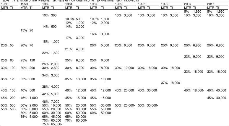
subject to progressive individual income tax. The transition of the marginal tax rates of
individual income tax is described in Table 1. This table shows that after WWII, the tax
system became more progressive until the 1970s and then became flatter until the 2000s.
Recently, it has become more progressive again.
Table 1 is inserted around here.
Local income tax, which has been much flatter than individual income tax and is currently a
completely flat tax, shares a similar tax base and is levied on the same individuals
repeatedly.9 It employed a progressive tax system with rates of 4–18% until 1986, but then
gradually became flatter and it is now a 10% flat tax.
9 Rigorously speaking, the deduction on national income tax is slightly different from that on
local income tax. For example, consider a salaried worker with an aggregate gross income
(AGI) of 6 million JPY with a housewife and two dependent children. His deduction on
national income tax in 1989 was at least 3.095 million JPY (employment income deduction
While the income tax system in Japan is similar to that in the United States, there are several
differences between them. Firstly, this tax is imposed on individual income, not on household
income. Secondly, although tax filing is in principle required for most people, a great
majority of people are exempt from this requirement. Notably, salaried workers typically pay
their taxes without filing because their employers file their taxes on their behalf; specifically,
salaried workers whose income is below 20 million yen do not have to file their own tax
return. Thirdly, people in the United States choose between two deduction strategies,
itemized deduction and standard deduction, whereas in practice, people in Japan do not have
such a choice. In Japan, the employment income deduction, similar to the standard deduction
in the United States, is applicable to salaried workers; salaried workers are able to choose the
itemized deduction strategy instead of legitimately calculated employment income deduction.
However, itemized deduction hardly exceeds employment income deduction; for example,
only four people in 2011 and six people in 2012 chose itemized deduction.
2.2 Tax Reform in the 1980s
dependent deduction 350 thousand ×2), whereas his deduction on local income tax in 1989
was at least 2.815 million JPY (employment income deduction 1,695 thousand + basic
deduction 280 thousand + spouse deduction 280 thousand + dependent deduction 280
thousand ×2). Therefore, the present study ignores the differences between them (see, for
As explained in the Introduction, similar to the experiences of most OECD countries during
the 1980s, Japan reduced its individual income tax rates as well as the number of brackets in
this decade. For instance, the top marginal tax rate of individual income tax decreased from
70% in 1984 to 50% in 1987, while the tax brackets were simplified from 15 in 1984 to five
brackets in 1987. Local income tax, having been much flatter than national income tax, also
experienced a similar reform during the 1980s. For high taxpayers, however, local income tax
has been almost a flat tax. It was 16–18% in 1986, 16% in 1987, and 15% in both 1988 and
1989. These tax rate changes before and after the reform are shown in Table 1.
3. Empirical Strategy
3.1 Econometric Specification
To estimate the ETI, we employ the conventional estimation model developed by Gruber and
Saez (2002). Specifically, the regression equation is expressed as follows:
log = + log 1 −1 − + log + + + ,
= 1, . . , , = 1986, … , 1988, (1)
where is the taxable income of individual in year and is that in year + 1. is
the marginal tax rate of the tax scheme in year and represents a vector of the other
control variables. The dependent variable is the difference in the log of taxable income
between years + 1 and . The first explanatory variable, to which we pay most attention
among the covariates, is the difference in the net-of-tax rate, thereby suggesting that is the
ETI with regard to the net-of-tax rate 1 − . The log of taxable income is included in the
income, in line with previous research. The vector of the other controls comprises a sex
dummy that takes the value of one for men, which captures the variation arising from
differences in sex and is conventionally employed in this type of estimation. Occupation
dummies are also adopted as a control in one regression. As explained later, using occupation
as a control copes with the heterogeneity in income trend and mitigates endogeneity bias in
the estimation compared with the standard IV estimation (Carroll, 1998; Auten and Carroll,
1999; Singleton, 2011; Weber, 2014). stands for the year dummy and is an error. The
coefficients of the explanatory variables are given by , , and . The definitions and units of
the variables are presented in Table 2.
Table 2 is inserted around here.
Eq. (1) is mainly estimated by using the 2SLS because of the emergence of endogeneity
between the log change in taxable income and that in the net-of-tax rates. In the ETI literature,
there is concern that the estimate of elasticity appears to be biased because of the presence of
a progressive taxation, which yields a positive correlation between realized income and
the marginal tax rate 1 − after controlling for the other covariates. To address this
concern, using the mechanical change in the tax rate structure (caused by the tax policy
reform) as an instrument has been suggested, which is created by applying the post-reform
tax schedule in year + 1 to pre-reform taxable income in year in order to isolate the
mechanical effect of the net-of-tax rate from the behavioral response of taxpayers to a tax
correlated with the predicted log change in the net-of-tax rate (Gruber and Saez, 2002);10 to
control for this endogeneity, the log of taxable income is included in an estimation equation,
as seen on the RHS of Eq. (1).
3.2 Identification Problems
Regarding the heterogeneous effects of pre-reform income on income growth, two potential
factors are argued in this literature. The first is mean reversion.11 Mean reversion entails bias
for an elasticity estimate, although the direction of the bias depends on whether pre-reform
incomes are larger or smaller than those on average. Mean reversion can be controlled for by
using one-year lagged income (here defined as log ) as a proxy. The second is a change in
income distribution. In the United States, income inequality has widened over the past three
decades, notably in the 1980s (Giertz, 2007). Turning to Japan, Moriguchi and Saez (2008)
provide evidence that top wage income shares remained relatively stable from 1980 to 1997
(see their Figures 10 and 11). Some of the studies cited in their Figure 2, however, indicate
that the Gini coefficients increased slightly from 1986 to 1989. The possibility of widening
inequality over time might thus be present, even in Japan.
10 This is because the income growth of each individual can vary by her/his income level,
which is positively associated with the change in the marginal tax rate under a progressive tax
schedule.
11 This is that if high (low) income is realized in the current period relative to the average, it
In this case, one solution is to incorporate the log of lagged taxable income as a control.
However, if income change occurs nonlinearly, this approach does not explain income
growth well. Another is to exploit a spline regression with regard to the log of the base year
income (e.g., Gruber and Saez, 2002). Several studies have employed a 10-piece spline in
their ETI estimations, while fewer researchers have used a lower piece spline, such as a
five-piece (Weber, 2014). Related to the choice of spline number, previous researchers employ
samples of lower-income as well as high-income taxpayers by setting the sampling thresholds
as above 15,000 USD (Auten and Carrol, 1999) or above 10,000 USD (Giertz, 2007; Gruber
and Saez, 2002). However, given that our database is composed of quite high taxpayers with
at least approximately 28 million JPY (about 280 thousand USD) taxable income, setting
many splines would seem to be unsuitable. For example, Weber (2014) employs a five-piece
spline while the employed taxable income threshold is 100 thousand USD (which is much
smaller than ours). This study thus adopts a four-piece spline to capture heterogeneous
changes in income growth as a robustness check.
In practice, the use of lagged taxable income or its spline as a proxy for income growth in the
regression raises some concerns. Weber (2014) points out that if the log of one-year lagged
(current year in this study) taxable income is used as a proxy for income growth, permanent
income remaining in the error term after controlling for transitory income by taking the log of
lagged taxable income is associated with lagged income. Since this correlation biases an ETI
temporary variation in income is needed. The present study adopts occupation dummies as
additional proxies in the robustness check. 12,13
Another substantial concern about the estimation of the ETI is the diverse definitions of
taxable income. In many large-scale tax reforms, tax rates are changed along with changes in
deductions, which makes it difficult to assess the effects of a change in the tax rate precisely.
In general, broader deductions and/or exemptions lead to a large estimate of the ETI
(Slemrod and Kopczuk, 2002; Saez et al., 2012; Slemrod, 1995). In the United States,
changes in deductions and exemptions affect the relative prices of itemizing activities for
taxpayers, making them alter their itemization status. Even when deductions remain
unchanged, a change in tax rates could affect tax filing behavior through a change in the
relative prices of tax benefits such as charitable deductions (Kopczuk, 2005; Slemrod and
12 Weber (2014) argues that unless the log of lagged taxable income is included in an
estimation equation, occupation or education level variables cannot proxy for transitory
income, resulting in a failure to solve the endogeneity. By contrast, the present study takes
the estimation strategy that including a lagged taxable income as a proxy for a transitory
income, the remaining error of a permanent income is controlled for by the occupation
variable.
13 The dummies are classified into the following categories: president, executive advisor, vice
president, board member, administrative officer, hospital director, doctor, dental manager,
dentist, school manager, professor, law and accounting office manager, lawyers and
accountants, chief priest, entertainer, sport player, artist, agriculture worker, public official,
Kopczuk, 2002). Kopczuk (2005) states that half of the behavioral responses of taxpayers to
the Tax Reform Act of 1986 can be accounted for by the response to broadening tax bases
and half by the response to reductions in tax rates. To cope with this problem, existing studies
estimate the elasticity of broad income in place of that of taxable income, demonstrating that
broad income elasticity is significantly smaller than the ETI (Giertz, 2007; Kopczuk, 2005).
Turning to the Japanese tax reform during 1986–1988, no choice over deduction strategies is
substantially available, as explained in Section 2. In addition, commodities deductible from
income, such as medical expenses and charitable contributions, were rarely available for
Japanese top income earners relative to the United States. At that time, top income earners
did not have a culture of making charitable giving, which can be viewed one of the most
crucial reasons to a behavioral response to tax changes, in contrast to the United States.14 In
addition, preferable tax treatment such as deduction is mostly limited to commodities
unlikely to be manipulated such as medical expenses, expenses for earthquake damages, and
so on, and for most deductions the upper ceilings are present. Overall, the use of Japanese tax
return data allows us to remove the bias caused by behavioral responses, specifically
itemization behavior, from the ETI estimates.
14 Charitable donations subject to taxable deduction were approximately 0.01% of GDP
(Statistics of National Tax Authority). Total charitable donations, including those that were
not claimed deduction, were still less than 0.1% of GDP (Family Income and Expenditure
Survey). Note that there is a great contrast to United States situation, where charitable
By contrast, a variation in the tax base arising from a change in the size of deductions, not
including a change from any behavioral response—an effect of the changes in deduction
size—appears under the Japanese income tax system. Because taxpayers experienced a tax
rate cut and a tax base narrowing at the same time in the Japanese tax reform, their marginal
tax rates became lower than without any change in the tax base, holding other things constant.
Thus, we should control for this “size” effect to ensure a consistent estimation of the ETI,
such as by using broad income instead of taxable income or adding the overall change in the
deduction into the empirical equation.
Nevertheless, a variation in deductions due to the Japanese tax reforms does not strongly
affect the estimation of the ETI. Assuming a behavioral response to a deduction change is not
present, the change in deduction appears as the ratio of a change in the deduction to current
taxable income. Following the theoretical model developed by Gruber and Saez (2002), the
size effect is expressed as follows:
log = log(1 − ) − , (2)
where denotes taxable income, is the marginal tax rate, and is the deduction. The
derivation of Eq. (2) is presented in Appendix A. Analogous to Eq. (1) of Gruber and Saez
(2002), log is the percentage change in taxable income, log(1 − ) is that in the
marginal tax rate, and represents the compensated elasticity of taxable income. A change
in the applied deduction relative to taxable income, / , represents the impact of the
change in deduction in our regression. For our sample of extremely high taxpayers, this ratio
children and earning an AGI of 50 million JPY, the ratio is about 0.002.15 We could thus
ignore the expansion of deductions in our estimation. Although there remains the potential for
bias from changes in the tax base, this possibility seems to be negligible because such a
change in deductions affects high taxpayers almost uniformly.
4. Data
The current study employs panel data on top taxpayers in Tokyo, Japan from 1986 to 1989,
named TheList of Top Taxpayers. The Japanese tax authority publicly notified high-income
taxpayers from 1950 to 2005, and the name, address, and taxable income (until 1982) or tax
liability (after 1982) were publicly posted on the boards of tax offices for a certain duration.
Approximately 70–110 thousand people were subject to such a notification each year during
the study period, of which about 120 million people lived in Japan. Although taxpayers with
a tax liability of more than 10 million JPY (about 100 thousand USD) are contained in the
original data, we focus on those who were reported in the lists from 1986 to 1989 and who
15 Her/his deduction in 1986 was at least 5,415 thousand JPY (employment income deduction
4,095 thousand + basic deduction 330 thousand + spouse deduction 330 thousand +
dependent deduction 330 thousand ×2), whereas her/his deduction in 1989 was at least 5,495
thousand JPY (employment income deduction 4,095 thousand + basic deduction 350
thousand + spouse deduction 350 thousand + dependent deduction 350 thousand ×2) (see, for
lived in Tokyo during this period.16,17 The income tax liabilities of the reference year and of
the previous year are listed in the list if incomes or tax liabilities in both years are above the
threshold for public disclosure. We then sampled the taxpayers reported in the top taxpayer
lists in 1987 and 1989 and whose incomes in 1986 and 1988 were also reported, respectively,
in the 1987 and 1989 lists. From this sampling procedure, a four-year panel dataset of top
taxpayers was constructed, which consisted of their income tax liabilities, name and address
(collected from the Japanese public notification records), and occupation.
The occupation variable contains information about types of jobs and company names for
executives if the main incomes of respondents come from the described occupation and/or
company. Then, limiting the sample to taxpayers of a certain occupation allows us to focus
on those respondents whose main incomes came from labor income. Although labor and
capital incomes are not completely distinguishable in our dataset, capital income accounts for
only a small share of the AGI under the Japanese personal income tax at that time. 18 Thus
16 The lower bonds of normalized taxable income to sample are approximately 34 million
JPY in 1986, 33 million JPY in 1987, 32 million JPY in 1988 and 28 million JPY in 1989.
17 We restricted the sample to Tokyo because a sufficient number of observations is available
from Tokyo and collecting data on all top taxpayers in Japan is very difficult. Additionally,
by restricting the location of taxpayers, it is possible to make conditions other than what is
obtained from the data, such as regional economy and a change in real estate price,
homogeneous.
18 Many previous studies isolate and then eliminate capital income from the income data in
including capital income in the AGI does not likely matter in the regressions of this study. As
a robustness check, however, we estimate by choosing a sample of executives only, who are
expected to earn most of their income from working as they were listed in the top taxpayer
lists for several years. Because sex is not reported in the original data, our sex data are
created by reference to the respondents’ names, which can be used in Japan to identify sex in
most cases. Taxpayers for which we could not discern their sex are omitted from the dataset.
Panel data are constructed by matching the surname, given name, and address between the
1987 and 1989 top taxpayer lists.19
2007; Weber, 2014). In our dataset, although capital income may be included in AGI, the
share of capital income could be quite small. First, as stated earlier, the sample employed in
estimation is limited to the taxpayers whose main incomes are from labor income. Second,
almost all interest income and most dividend income were subject to a separate withholding
tax and thus not included in AGI. To be precise, Iwamoto et al. (1995) reveal that almost all
interest income (specifically, more than 99.75%) was either subject to a separate withholding
tax or exempt from taxation during the period we are interested in, in which most dividend
income was subject to a separate withholding tax and thus only 20-30% of dividend income
was included in AGI. Third, real estate transfer income was generally subject to a separate
tax, too; capital gains were not taxed until 1988 and, after then, subject to a separate
withholding tax. Other capital income such as real property income, however, was included
in AGI.
19 Because some high taxpayers have the same surname and given name, we use address as
well to identify them correctly. Hence, we omit listed taxpayers who moved to another
One concern about the dataset is the attrition of observations. The current strategy to create
the database requires that selected taxpayers keep paying more than 10 million JPY income
tax for four consecutive years, indicating that the proportion of the sample around the
threshold is less dense than the actual income distribution. To deal with this problem, as a
robustness check, we omit those who could have possibly dropped off the top taxpayer lists in
each year. Specifically, we first estimate kernel density functions for each year to identify the
maximums of the densities. As the extremely high income distribution in Japan typically
follows a Pareto distribution20 (e.g., Hasegawa et al., 2013; Souma, 2001), some taxpayers
whose taxable incomes are below the maximum of the kernel density are omitted from the
samples. Hence, Pareto density functions for every year are estimated by using taxpayers
with taxable incomes above the maximum kernel density. Finally, we exclude from our
sample taxpayers whose taxable incomes fall in the range where the Pareto probability
densities are 10% greater than the kernel densities.21 In the taxable income range where the
Pareto densities are apparently greater than the kernel ones, attrition may occur. By setting
the cut-offs below which the sample is omitted based on difference between the estimated
20 Souma (2001) and Aoyama et al. (2011) point out that taxable income above about 20
million yen follows a Pareto distribution. Since the lower bound of the List of Top Taxpayers
is well above this threshold, we can safely assume that the income distribution of our data
should follow a Pareto distribution.
21 The thresholds of taxable income to omit lower taxpayers are 46 million JPY in 1986, 45.7
million JPY in 1987, 42.1 million JPY in 1988, and 39.2 million JPY in 1989. The average
Pareto and kernel densities, we attempt to mitigate any bias from attrition in the regression.22
The figures of the kernel density and Pareto distribution for every sample year and the related
comments are provided in Appendix B.
Table 3 is inserted around here
Figure 1 is inserted around here
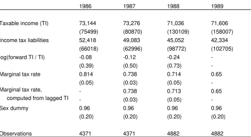
Table 3 presents the descriptive statistics of the data used in the estimation. Taxable incomes
and tax liabilities are normalized by taxable income in 1989; the marginal tax rates are
computed for the normalized taxable income and brackets of national and local income taxes.
The log difference in taxable income, the marginal tax rates and those computed from lagged
taxable income are quantified by using the weights of real taxable income. We see that on
average, taxable incomes remain stable over time, whereas tax liabilities decrease steadily;
indeed, the averages of marginal tax rates for our sample drop from about 81% to 65%. Since
both the marginal tax rates and the number of brackets for high-income earners reduced in
1989, all the taxpayers in our sample faced the same marginal tax rate and the same one
22 Since the top taxpayers list consists of tax file data submitted by March 31, some attrition
from this list may be caused by delaying the tax filing. According to Hasegawa et al. (2013),
approximately 1% of high taxpayers may have been dropped from this top taxpayers list,
most of who were close to the threshold. We address this possible attrition as well by
predicted from the lagged taxable income, 65%. Finally, the sex dummy shows that most
sampled taxpayers are men.
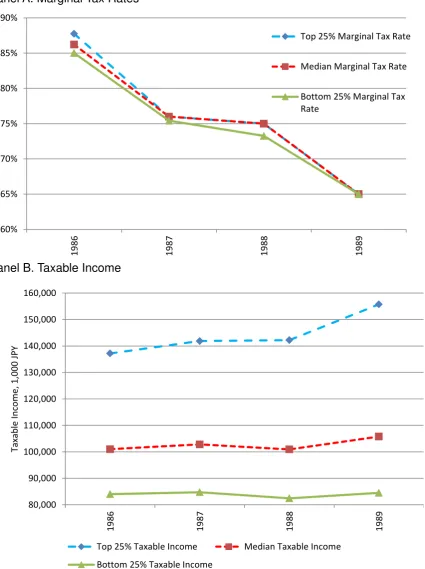
Figure 1 illustrates the average marginal tax rates (weighted by taxable income) and the
average taxable incomes for the top 25%, median (top 50%), and bottom 25% taxpayers in
our sample. As shown in Panel A, the average marginal tax rates for all taxpayers fell from
around 86% to 65% in the sample period, showing a larger drop for higher taxpayers. By
contrast, their taxable incomes increased over time; more specifically, taxpayers with higher
taxable incomes rose largely, suggesting that taxpayers who faced a large decline in marginal
tax rates are likely to increase their taxable incomes. This graphical evidence is in line with
that of Kleven and Schultz (2014) and infers the existence of the positive ETI.
5. Estimation Results
5.1 Baseline Estimation
Table 4 is inserted around here
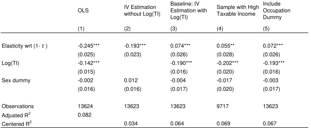
Table 4 provides the estimation results of the elasticity of taxable income with regard to the
net-of-tax rates, using tax return data on top taxpayers in Japan. The OLS regression in
column (1) shows a negative coefficient of the ETI, which is inconsistent with the intuitive
Saez, 2002; Saez et al., 2012). The IV estimation excluding the log of taxable income, which
can be used as a proxy for heterogeneous income growth as discussed above, in column (2)
shows that the growth in taxable income is negatively and significantly correlated with that of
the net-of-tax rate. Most previous empirical works have reported the same result, thus
indicating that these counterintuitive results may reflect well-known problems with the
econometric specification of income growth (e.g., Kleven and Schultz, 2014; Weber 2014).
Column (3) is our baseline regression. The IV regression with the log of taxable income
being included provides a positive estimate of the ETI, supporting the existence of a positive
elasticity with regard to the net-of-tax rate. The size of the ETI is about 0.074, which is
smaller than earlier estimates, such as 0.4 in the 1980s of the United States by Gruber and
Saez (2002), 0.26 in the 1990s in the United States (Giertz, 2007), and 0.5–0.6 by Saez et al.
(2012); however, it is similar to others such as 0.06 (Kleven and Schultz, 2014). The estimate
of the log of taxable income appears significant and negative, and its point estimate is close
to previous ones such as -0.167 (see Table 4 of Gruber and Saez, 2002) and -0.165 (see Table
5 of Giertz, 2007). The sex dummies are all not strongly significant with small point
estimates.
As in column (4), omitting low-income taxpayers by setting the thresholds at 39–46 million
JPY does not change the ETI estimate dramatically, with an 0.055 point estimate of the ETI.
In column (5), we incorporate the occupation dummies as controls to address the endogeneity
problem stemming from the correlation between permanent income and income level. This
It follows that, as seen in columns (3)–(5), the ETI for Japanese top taxpayers is around
0.074–0.055. One reason for this relatively small estimate is that the standard deduction for
salaried workers in Japan (i.e., the employment income deduction) is generous23 to the point
that few salaried workers choose an itemized deduction instead of a standard deduction. It
seems that partly because taxpayers have no choice of deduction, the ETI in Japan is less than
that in the United States, where almost half of the ETI can be explained by the choice of
deductions (Slemrod and Kopczuk, 2002; Kopczuk, 2005). Because of the disadvantage of
the ETI in terms of deduction choice, recent ETI studies have estimated broad income
elasticity; however, as stated above, broad income elasticity is not comparable with the ETI
estimates obtained in previous studies as broad income is much bigger than the corresponding
taxable income. Thus, the ETI estimates free from bias from the possibility of deduction
choice give some novelty and insight in this literature.
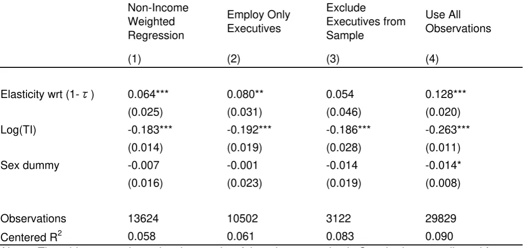
5.2 Robustness Check and Extended Estimation
The results for the robustness checks are provided in Table 5. Giertz (2007) argues that an
ETI estimate is sensitive to income weighting in the regressions: specifically, the absence of a
broad or taxable income weight remarkably decreases estimates of the ETI compared with
23 The standard deduction in Japan (i.e., the employment income deduction) for salaried
workers increases with one’s salary, whereas the standard deduction for US taxpayers is
constant. Moreover, the standard deduction for high-earning Japanese workers is more than
those estimated with these weights, although standard in this literature. We thus model a
regression without a taxable income weight and obtain an ETI of 0.064 (see column (1)).
Table 5 is inserted around here
Another identification strategy for the problem about income data is to sample only
executives of companies. As shown in column (2), this regression yields a slightly large and
significant ETI estimate of 0.08. Conversely, as in column (3), eliminating the executives
from the sample leads to a smaller and insignificant estimate of 0.054. This finding suggests
that the ETIs estimated earlier are robust even if the issues on the definition of the income
variable are taken into account.
The estimation in column (4) utilizes the entire sample, including the high taxpayers omitted
because their tax liabilities fell below the thresholds of the top taxpayer lists in either of the
sample years, with more than twice the number of observations in the baseline. The
regression finds a significant and positive estimate of approximately 0.13, larger than that in
the baseline. Because this regression contains the sample excluded from the original, this
result is partly attributed to mean reversion, thereby yielding an upward bias of the estimate.
Overall, the regressions in the robustness check demonstrate that the ETI estimates are robust
to alternative specifications and sampling approaches and that the results in this table seem to
be in line with conventional arguments about the ETI, such as mean reversion (e.g., Saez et
Table 6 is inserted around here
The estimates of the other extended regressions are presented in Table 6. Column (1)
provides the coefficients from a spline regression and shows that the usage of a four-piece
spline instead of the log of taxable income lowers the ETI estimate to 0.046. However, this
result does not seem to be serious for the present analysis. Since the used data are composed
of extremely high taxpayers, their income growth trends are expected to be similar and thus
not necessarily controlled for by the splines.
Another argument regarding the ETI is the duration of a taxpayer’s behavioral response. As
discussed in Weber (2014), arbitrary choices of one-year or several-years difference in the
log of taxable income in the period when a tax reform is phased in may bias an ETI estimate.
Neither a short-term response—usually defined as a one-year difference—nor a long-term
one—more than a three-year difference—may measure the intended responses correctly
because several changes to a tax scheme may affect the responses in such a phased-in
duration. To deal with this problem, we assess the short-term response to the 1987 tax change
by taking the difference in the log of taxable incomes between 1986 and 1987 and the
long-term response by taking the difference between 1986 and 1989. As shown in columns (2) and
(3), the short-term response is 0.131, greater than the baseline estimate, and significant,
whereas the long-term one is quite small and insignificant. These findings support the
existence of a short-term response to the Japanese income tax reform, but not the emergence
6. Concluding Remarks
The current study estimates the ETI with regard to the net-of-tax rate, using data on Japanese
top taxpayers during 1986–1989. We pay close attention to the drastic tax reforms in 1987
and 1988, which diminished the top marginal income tax rates sharply and largely broadened
income tax deductions and exemptions, and estimate how taxpayers responded to the change
in the marginal tax rates in Japan.
The data on top taxpayers are four-year panel and tax return data, including demographic
information such as sex and occupation. One advantage of our dataset is that the Japanese
personal income tax provided no choice of standard or itemized deduction, which allows us
to estimate the elasticity of taxable income precisely. Another advantage is that the sample
period of the data covers the major income tax reforms and represents the period during
which the top income distribution in Japan remained stable. Although the standard estimation
approach in this literature is to adopt the “mechanical” effect of the net-of-tax rate as an IV
and the lags of taxable income as a control to address relevant econometric issues, other
empirical concerns arise for the current estimation: the correlation between lagged income
and permanent income, attrition from the top taxpayer lists, and definition of income. To deal
with these issues, we carried out regressions that included the occupation variables in the
estimation equation and restricted the sample to only extremely high taxpayers or executives
Based on the presented analysis, we find that the ETI with regard to the net-of-tax rate is
about 0.074–0.055 in Japan. Moreover, the ETI estimates of other approaches, such as
restricting the sample to extremely high-income earners, using a non-income weighting
regression, using occupation dummies, and adopting a four-piece spline of taxable income as
controls, are significant and positive with almost the same point estimate. Overall, we show
that the ETI for Japanese top taxpayers is smaller than those in Canada, Germany, Hungary,
Sweden, and the United States, but nearly equal to that in Denmark.
Nevertheless, there may be some caveats left in this study. One is that the elasticity of broad
income is not estimated. As recent studies have drawn attention to the estimation of broad
income elasticity because of the possibility of deduction choices (Chetty, 2009; Kopczuk,
2005), the estimation of the ETI and broad income elasticity and comparison between them
are preferable and insightful for this literature. This comparison, however, is impossible for
the present study because of the absence of broad income data. Another is that the ETI
obtained here is just a Japanese case. Although the small ETI estimates here appear because
the ETI, not broad income elasticity, is estimated and because of no choice of deductions in
Japan, other factors specific to Japan may generate this result, such as tax moral,
effectiveness of tax inspection, and so on. Further studies are needed to investigate the effects
of these factors.
Appendix A. Derivation of Eq. (2)
A taxpayer maximizes utility with regard to consumption, , and taxable (reported) income, ,
= ( − )(1 − ) + = (1 − ) + , where is pre-tax income and denotes virtual
income. From the maximization problem, we derive a reported income function, = (1 −
, , ), where the function depends on the net-of-tax rate, the deduction, and virtual income.
Taking the total derivative of with regard to , , and yields
= − (1 − ) + + . (3)
In the ETI literature, the uncompensated ETI with regard to the net-of-tax rate is represented
by = [(1 − )/ ] / (1 − ); the income effect is = (1 − ) / . From the budget
constraint, / = −1. Then, Eq. (3) is rewritten as
= − 1 − − + 1 − . (4)
By using the Slutsky equation = + and dividing both sides of Eq. (4) by , we obtain
= − 1 − − + (1 − ) . (5)−
Without the income effect and taking a logarithm form of this equation, Eq. (2) follows from
Eq. (5).
Appendix B. Figures of Kernel Density and Pareto Distribution
Figure A1 depicts the fitted curves of the kernel and Pareto densities as well as the
histograms of taxable income for 1986–1989. For every histogram, the densities of taxable
income peak between 30 million and 40 million JPY, above which they decline with taxable
does not hold at the low end of taxable income. As stated above, the thin densities at the low
income level may occur because of our sampling strategy (i.e., only taxpayers who appear in
the original data for all sample years are employed in the estimation).
Figure A1 is inserted around here
Moreover, the kernel density estimates of all panels mostly trace the densities of the
histogram with only one peak where taxable incomes are below 40 million JPY. By contrast,
the fitted Pareto densities exhibit a consistent downward sloping pattern. Below a taxable
income of 50 million, they exceed the corresponding kernel densities steadily and greatly as
taxable income declines, and the disparities between the Pareto densities and kernel estimates
appear the largest when taxable incomes are the smallest. Indeed, the comparison of the
Pareto and kernel densities highlights the remarkable attrition in our sample. As a robustness
References
Aarbu, Karl O. and Thor O., Thoreson, “Income Responses to Tax Changes—Evidence from
the Norwegian Tax Reform,” National Tax Journal 54(2) (2001), 319– 334.
Andreoni, James, “Philanthropy,” in S-C. Kolm and J. Mercier Ythier, eds., Handbook of
Giving, Reciprocity and Altruism, (Amsterdam: North Holland, 2006), 1201-1269.
Aoyama, Hideaki, Yoshi Fujiwara, Yuichi Ikeda, Hiroshi Iyetomi, and Wataru Souma,
Econophysics and Companies, Statistical Life and Death in Complex Business Networks
(Cambridge: Cambridge University Press, 2011).
Auten, Gerald E., and Robert Carroll, “The Effect of Income Taxes on Household Income,”
Review of Economics and Statistics 81 (1999), 681–693.
Blomquist, Sören, and Håkan Selin, “Hourly Wage Rate and Taxable Labor Income
Responsiveness to Changes in Marginal Tax Rates,” Journal of Public Economics 94
(2010), 878–889.
Cabinet Office Japan. 2001. “About the Effect of Tax Reform in 1990s.” Policy Effect
Analysis Report No. 9 (http://www5.cao.go.jp/keizai3/2001/1129seisakukoka9.pdf). (in Japanese)
Carroll, Robert, “Do Taxpayers Really Respond to Changes in Tax Rates? Evidence from the
1993 Tax Act.” U.S. Department of the Treasury Office of Tax Analysis Working Paper
79, 1998.
Chetty, Raj, “Is the Taxable Income Elasticity Sufficient to Calculate Deadweight Loss? The
Implications of Evasion and Avoidance,” American Economic Journal: Economic Policy
Doerrenberg, Philipp, Andreas Peichl, and Sebastian Siegloch, “The Elasticity of Taxable
Income in the Presence of Deduction Possibilities,” Journal of Public Economics (2015),
forthcoming.
Feldstein, Martin, “The Effect of Marginal Tax Rates on Taxable Income: A Panel Study of
the 1986 Tax Reform Act,” Journal of Political Economy 103 (1995), 551–572.
Giertz, Seth H., “The Elasticity of Taxable Income over the 1980s and 1990s,” National Tax
Journal 60 (2007), 743–768.
Giertz, Seth H., “Panel Data Techniques and the Elasticity of Taxable Income.” Proceedings.
Annual Conference on Taxation and Minutes of the Annual Meeting of the National Tax
Association 102, 102nd Annual Conference on Taxation (November 12-14, 2009), 77-87.
Gruber, Jon, and Emmanuel Saez, “The Elasticity of Taxable Income: Evidence and
Implications,” Journal of Public Economics 84 (2002), 1–32.
Hansson, Åsa, “Taxpayers’ Responsiveness to Tax Rate Changes and Implications for the
Cost of Taxation in Sweden,” International Tax and Public Finance 14 (2007), 563–82.
Hasegawa, Makoto, Jeffrey L. Hoopes, Ryo Ishida, and Joel Slemrod, “The Effect of Public
Disclosure on Reported Taxable Income: Evidence from Individuals and Corporations in
Japan,” National Tax Journal 66 (2013), 571-608.
Iwamoto, Yasushi, Yuichi Fujishima, and Norifumi Akiyama, “Evaluations and Issues about
Interest and Dividend Income Taxation,” Financial Review (1995), May, 1-24. (in
Japanese)
Kiss, Áron, and Pálma Mosberger, “The Elasticity of Taxable Income of High Earners:
Kitamura, Yukinobu, and Takeshi Miyazaki, “Elasticity of Taxable Income and Optimal Tax
Rate in Japan; Analysis by the Proprietary Data of National Survey of Family Income and
Expenditure,” Global COE Hi-Stat Discussion Paper Series No. 150, 2010. (in Japanese)
Kleven, Henrik Jacobsen, and Esben Anton Schultz, “Estimating Taxable Income Responses
Using Danish Tax Reforms,” American Economic Journal: Economic Policy 6 (2014),
271–301.
Kopczuk, Wojciech, “Tax Bases, Tax Rates and the Elasticity of Reported Income,” Journal
of Public Economics 89 (2005), 2093–2119.
Lindsey, Lawrence B, “Individual Taxpayer Response to Tax Cuts: 1824–1984: With
Implications for the Revenue Maximizing Tax Rates,” Journal of Public Economics 33
(1987), 173–206.
Moriguchi, Chiaki, and Emmanuel Saez, “The Evolution of Income Concentration in Japan,
1886–2005: Evidence from Income Tax Statistics,” Review of Economics and Statistics
90 (2008), 713–34.
Saez, Emmanuel, Joel Slemrod and Seth H. Giertz, “The Elasticity of Taxable Income with
Respect to Marginal Tax Rates: A Critical Review,” Journal of Economic Literature 50
(2012), 3–50.
Sillamaa, Mary-Anne and Michael R. Veall. “The Effect of Marginal Tax Rates on Taxable
Income: A Panel Study of the 1988 Tax Flattening in Canada.” Journal of Public
Economics 80 (3) (2001), 341–56.
Singleton, Perry, “The Effect of Taxes on Taxable Earnings: Evidence from the 2001 and
Slemrod, Joel, “Income Creation or Income Shifting? Behavioral Responses to the Tax
Reform Act of 1986,” American Economic Review 85 (1995), 175–180.
Slemrod, Joel, and Wojciech Kopczuk, “The Optimal Elasticity of Taxable Income,” Journal
of Public Economics 84 (2002), 91–112.
Souma, Wataru, “Universal Structure of the Personal Income Distribution,” Fractals 9 (2001),
463–470.
Weber, Caroline, “Toward Obtaining a Consistent Estimate of the Elasticity of Taxable
Income Using Difference-in-Differences,” Journal of Public Economics 117 (2014), 90–
103.
Yashio, Hiroyuki, “The Effect of Marginal Tax Rates on Taxable Income: The Case of
Business Income Earners in Japan,” The Hitotsubashi Review 134 (2005), 1135–1158. (in
Table 1. Transition of the Marginal Tax Rate of Individual Income Tax (National Tax), 1950-2015
1950 1953 1969 1984 1987 1989 1995 1999 2007 2015
MTR TI MTR TI MTR TI MTR TI MTR TI MTR TI MTR TI MTR TI MTR TI MTR TI
5% 1,950 5% 1,950
10% 300 10% 3,000 10% 3,300 10% 3,300 10% 3,300 10% 3,300
10.5% 500 10.5% 1,500 12% 1,200 12% 2,000 14% 600 14% 2,000
15% 20
16% 3,000 17% 3,000
18% 1,000
20% 50 20% 70 20% 5,000 20% 6,000 20% 9,000 20% 9,000 20% 6,950 20% 6,950
21% 4,000 22% 1,500
23% 9,000 23% 9,000
25% 80 25% 120 25% 6,000 25% 6,000
26% 2,000
30% 100 30% 200 30% 2,500 30% 8,000 30% 8,000 30% 10,000 30% 18,000 30% 18,000
33% 18,000 33% 18,000 34% 3,000
35% 120 35% 300 35% 10,000 35% 10,000
37% 18,000-38% 4,000
40% 150 40% 500 40% 12,000 40% 12,000 40% 20,000 40% 30,000 40% 18,000- 40% 40,000
42% 5,000
45% 200 45% 1,000 45% 15,000 45% 15,000 45%
40,000-46% 7,000
50% 500 50% 2,000 50% 10,000 50% 20,000 50% 30,000 50% 20,000- 50% 30,000-55% 500- 55% 3,000 55% 20,000 55% 30,000 55% 50,000
60% 5,000 60% 30,000 60% 50,000 60% 50,000-65% 5,000- 65% 45,000 65% 80,000
65,000-Variable Definition Unit
Taxable income (TI) Taxable income of individual income tax Thousand JPY
Income tax liabilities Tax liabilities computed from the taxable income by applying the progressive tax rates of the Japanese income tax
Thousand JPY
Marginal tax rate Marginal tax rate of income tax, computed from the taxable income; the marginal tax rate comprises an income tax rate and local tax rates for residents' income
Percentage
Marginal tax rate,
computed from lagged TI
Marginal tax rate calculated by applying the income tax rate of the current year to one-year lagged taxable income
Percentage
Sex dummy A dummy that takes the value one for men
-Occupation dummies Dummies for specific occupations: president, executive advisor, vice president, board member, administrative officer, hospital director, doctor, dental manager, dentist, school manager, professor, law and accounting office manager, lawyers and accountants, chief priest, entertainer, sport player, artist, agriculture worker, public servant, politician, businessman
-Notes: The table reports the definitions and units of the dependent and explanatory variables and related variables. One JPY is equal to approximately 0.01 USD. All variables are sourced from The List of Top Taxpayers in 1986-1989.
Table 3. Descriptive Statistics, 1986–1989
1986 1987 1988 1989
Taxable income (TI) 73,144 73,276 71,036 71,606
(75499) (80870) (130109) (158007)
Income tax liabilities 52,418 49,083 45,052 42,334
(66018) (62996) (98772) (102705)
log(forward TI / TI) -0.08 -0.12 -0.24
-(0.39) (0.50) (0.73)
-Marginal tax rate 0.814 0.738 0.714 0.65
(0.05) (0.03) (0.05)
-Marginal tax rate, - 0.738 0.713 0.65
computed from lagged TI - (0.03) (0.05)
-Sex dummy 0.96 0.96 0.96 0.96
(0.20) (0.20) (0.20) (0.20)
Observations 4371 4371 4882 4882
OLS IV Estimation without Log(TI)
Baseline: IV Estimation with Log(TI)
Sample with High Taxable Income
Include Occupation Dummy
(1) (2) (3) (4) (5)
Elasticity wrt (1-τ) -0.245*** -0.193*** 0.074*** 0.055** 0.072***
(0.025) (0.023) (0.026) (0.028) (0.026)
Log(TI) -0.142*** -0.190*** -0.202*** -0.193***
(0.015) (0.016) (0.020) (0.016)
Sex dummy -0.002 0.012 -0.004 -0.017 -0.003
(0.016) (0.016) (0.017) (0.020) (0.017)
Observations 13624 13623 13623 9717 13623
Adjusted R2 0.082
Centered R2 0.034 0.064 0.069 0.067
[image:41.842.36.662.74.332.2]Notes: The table reports the estimation results of the ETI with regard to the net-of-tax rate, using panel data on Japanese top taxpayers from 1986 to 1989. Standard errors adjusted for clusters are in parentheses; *, **, and *** denote significance at 10%, 5%, and 1%, respectively. Every estimation includes year dummies, and is weighted by the log of taxable income. Basically, the sample is restricted to individuals listed in The List of Top Taxpayers in the four years and whose main income came from working. Column (4), however, adopts an alternative sample, which is restricted to extremely high taxpayers who are expected not to drop out of the sample during the sample period.
Non-Income Weighted Regression
Employ Only Executives
Exclude
Executives from Sample
Use All Observations
(1) (2) (3) (4)
Elasticity wrt (1-τ) 0.064*** 0.080** 0.054 0.128***
(0.025) (0.031) (0.046) (0.020)
Log(TI) -0.183*** -0.192*** -0.186*** -0.263***
(0.014) (0.019) (0.028) (0.011)
Sex dummy -0.007 -0.001 -0.014 -0.014*
(0.016) (0.023) (0.019) (0.008)
Observations 13624 10502 3122 29829
Centered R2 0.058 0.061 0.083 0.090
[image:42.595.39.552.74.317.2]Notes: The table reports the estimation results of the robustness check. Standard errors adjusted for clusters are in parentheses; *, **, and *** denote significance at 10%, 5%, and 1%, respectively. Every estimation includes year dummies, and is weighted by the log of taxable income except for column (1) (where no weights are used). The sample of column (2) is restricted to the top taxpayers who worked as an executive, whereas that of column (3) is restricted to those who did not work as it. Column (4) uses all the samples collected in our study.
4-Piece Spline Short-term
Response, 1986-87
Long-term
Response, 1986-89
(1) (2) (3)
Elasticity wrt (1-τ) 0.046* 0.131** 0.009
(0.026) (0.056) (0.066)
Log(TI) -0.175*** -0.194***
(0.031) (0.044)
Sex dummy -0.008 -0.017 0.035
(0.017) (0.029) (0.031)
1st spline -0.317*** (0.061)
2nd spline -0.217*** (0.054) 3rd spline 0.120***
(0.043) 4th spline -0.291***
(0.034)
Observations 13623 4371 4371
[image:43.595.40.494.80.462.2]Centered R2 0.078 0.028 0.047
Table 6. Extended Estimation of the ETI with regard to the Net-of-Tax Rate
Notes: The table reports the results of the other relevant regressions of the ETI. Standard errors adjusted for clusters are in parentheses; *, **, and *** denote
Figure 1. Marginal Tax Rates and Taxable Income for the Top 25%, Median (top 50%) and Bottom 25% Taxpayers
Panel A. Marginal Tax Rates
Panel B. Taxable Income
60% 65% 70% 75% 80% 85% 90% 19 86 19 87 19 88 19 89
Top 25% Marginal Tax Rate
Median Marginal Tax Rate
Bottom 25% Marginal Tax
Rate 80,000 90,000 100,000 110,000 120,000 130,000 140,000 150,000 160,000 19 8 6 19 8 7 19 8 8 19 8 9 Taxable In come, 1 ,000 JPY
Top 25% Taxable Income Median Taxable Income
Figure A1. Histogram, Kernel Density, and Fitted Pareto Density of Taxable Income, 1986– 1989
Panel A. Year 1986
Panel B. Year 1987
0 2. 0e -0 5 4. 0e -0 5 6. 0e -0 5 8. 0e -0 5 1. 0e -0 4 De ns it y
30000 40000 50000 60000 70000 80000 90000 100000 Taxable income, thousand JPY
Histogram
Kernel density estimate Fitted Pareto density
0 2. 0e -0 5 4. 0e -0 5 6. 0 e -0 5 8. 0e -0 5 De ns it y
30000 40000 50000 60000 70000 80000 90000 100000
Taxable income, thousand JPY
Histogram
Panel C. Year 1988
Panel D. Year 1989
0 2. 0e -0 5 4. 0e -0 5 6. 0e -0 5 8. 0e -0 5 1. 0e -0 4 De ns it y
30000 40000 50000 60000 70000 80000 90000 100000 Taxable income, thousand JPY
Histogram
Kernel density estimate Fitted Pareto density
0 2 .0e -0 5 4. 0e -0 5 6. 0e -0 5 8. 0e -0 5 1. 0e -0 4 De ns it y
30000 40000 50000 60000 70000 80000 90000 100000
Taxable income, thousand JPY
Histogram