A Derivative Free Optimization Algorithm Using Sparse Grid Integration

A Derivative-Free Optimization Algorithm Using

Sparse Grid Integration

Shengyuan Chen, Xiaogang Wang

Department of Mathematics and Statistics, York University, Toronto, Canada Email: [email protected], [email protected]

Received October 2, 2012; revised November 12, 2012; accepted December 1,2012

ABSTRACT

We present a new derivative-free optimization algorithm based on the sparse grid numerical integration. The algorithm applies to a smooth nonlinear objective function where calculating its gradient is impossible and evaluating its value is also very expensive. The new algorithm has: 1) a unique starting point strategy; 2) an effective global search heuristic; and 3) consistent local convergence. These are achieved through a uniform use of sparse grid numerical integration. Numerical experiment result indicates that the algorithm is accurate and efficient, and benchmarks favourably against several state-of-art derivative free algorithms.

Keywords: Nonlinear Programming; Derivative Free Optimization; Sparse Grid Numerical Integration; Conditional Moment

1. Introduction

Derivative-based methods can be very efficient and have been widely used in solving optimization problems. In many applications, however, the derivative of an object- tive function might be unavailable, unreliable, or very costly to compute. Many scientific and engineering op- timization problems fall into this category [1]. For exam- ple, in the helicopter rotor blade design problem [2], the objective function can only be evaluated by very expen- sive simulation. Similar problems include the nonlinear optimization parameter tuning problem [3], medical im- age registration [4], dynamic pricing [5], and community groundwater problem [6]. Therefore, derivative-free me- thods must be used in these situations. For these prob- lems, not only the derivative information is not available, the function evaluation could be inaccurate or noisy most of times as well. Hence, an algorithm needs the capabil- ity to generate robust searching directions without using derivative and without overly relying on individual func- tion evaluations.

There are several commonly used derivative-free algo- rithms in the literature. The classical Nelder-Mead me- thod [7] is based on simplicies and various operations defined on these simplicies. The method evaluates the objective function on a finite number of points, and de- cides which operation to perform accordingly. The me- thod is simple and able to follow the curvature of the objective function. Pattern search or directional direct search algorithm [8,9] defines a set of directions before-

hand, such as positive spanning sets, positive bases or just the coordinates in its simplest form, and tests one candidate point on each of these directions in a so called polling step. An optional search step could proceed the polling step to accelerate the algorithm opportunistically, in which the algorithm makes use of some known prop- erties, heuristics, or a surrogate model on a finite number of points. The implicit-filtering method [10] is a line search method based on the simplex gradient, which is computed based on the function values at the vertices of a simplex set. DFO method [11], Powell’s method [12] and Wedge method [13] are essentially trust-region methods; however, additional steps are executed since in the derivative free optimization a quadratic or linear in- terpolating or regression model does not necessarily im- prove when the trust-region radius is reduced. For ex- treme problems where the mathematical structure is complex or poorly understood, other heuristic optimiza- tion algorithms such as genetic algorithms, simulated annealing, artificial neural networks, tabu-search and particle swamp are also used as methods of a last resort. An excellent discussion of several commonly used de- rivative-free optimization methods can be found in [14].

cases like the helicopter rotor blade design problem [2], where each function evaluation is an expensive simula-tion and is known to be noisy, generating robust and effi-cient searching directions has the highest priority. It does not mean that one can not conduct derivative-free global optimization. As a matter of fact, many derivative-free global optimization algorithms have been developed with different targeted application areas, for example, the par- ticle swarm method, Mesh adaptive direct search (MADS) [15], DIviding RETangles (DIRECT) [16], and Multileve coordinate search (MCS) [17]. More interestingly, some of the above local derivative-free algorithms have been extended to solve global optimization problems, for example, the global Direct Search, see Section 13.3 [14] and references therein. It appears that four categories of algorithms, with or without derivative, seeking local or global optimums, all find their suitable application ar- eas.

In this paper, our goal is to generate high-quality local optimal solutions efficiently. Hence in this paper, we are concerned with the following optimization problem:

 

max ,

x B f x (1)

where

 

_: d 2

f   C , but is expensive to evaluate. In many applications, such as the helicopter rotor blade design problem [2], f

 

 nown to be smooth, but has no analytical form, and one can only rely on expen-sive simulations or experiments to evaluate function val-ues. The measurements could be inaccurate or noisy though the function

is

 

k

f 

 

itself is known to be smooth, see [14]. Furthermore, derivatives or reliable approxima-tion are not available. f  could have many local op-timums as well. The decision variable x is subject to a box constraint xB. For example, in the parameter tubing problem [3], B is a theoretically or empirically reasonable range of the parameters to be tuned.

Our research is motivated by Wang et al. [18], where the authors proposed a novel derivative free global opti-mization method. In this iterative method, the integral of the objective function over a local neighbourhood of each iterate is computed, which further determines the next iterate. The authors showed that if the neighbour-hood size could be chosen properly at each iterate, the algorithm converges to a global optimum. The authors demonstrated a few examples, where the algorithm suc- cessfully found global optimums while several other commonly used derivative-free methods and even deri- vative-based methods failed.

We have a different view of the integration based de-rivative free optimization method. First of all, we use the integration to define the searching directions, rather than the iterates as did in [18]. We found that it is more effi-cient to use the integration to define the search direction. The integration based searching direction uses

informa-tion from multiple funcinforma-tion evaluainforma-tions at strategically located points, which avoids unduly relying on the gra-dient information at the current iterate. This is especially important since the function evaluations are noisy, espe-cially when obtained from simulation or physical meas-urements, hence the local gradient, even if available or can be approximated, has poor quality. Secondly, our focus is on generating high quality local optimum effi-ciently, rather than seeking a global optimum. This mod-erate goal actually enable us to search more effectively. Finding global optimum and proving its global optimality is known to be hard. Though [18] shows the existence of a series of neighbourhood sizes such that their algorithm can find a global optimum, the exact neighbourhood size is not given in theory, nor specified algorithmically. In this paper, we design a two stage searching strategy, which aims at achieving a good balance of global cover-age and local optimality.

First, we divide the solution seeking process into two stages: the global probing stage and the local conver-gence stage. In the global probing stage, the algorithm search for high region of the feasible domain for a maximization problem; while in the local convergence stage, the algorithm converges to peaks of the high re- gion found in the first stage. The first stage steps are typically large; and the second stage steps are small. We update the neighbourhood size differently in the two stages, which suites the different purposes of the two stages well.

Accordingly, we prove that in the local convergence stage the algorithm always generates locally improving directions and converges; while in the global probing stage, we are able to show that the algorithm can gener- ate searching directions towards a global optimum but against a local attraction for the mixture model functions commonly appeared in statistics optimization.

We not only develop new theories to support our new perspective, but also design critical algorithmic compo-nents accordingly. Our new line search method is a greedy algorithm which appears to have good numerical performance. In the contrast, [18] does not use line search at all. Our strategy to select the starting point is also new. It is well-known that the starting point is im-portant for nonlinear optimization problem. However, most nonlinear optimization algorithms, including [18], rely on user defined starting points or starting from zero mechanically. We provides an innovative approach here: we start from the center of gravity of the whole feasible region, which is again computed from integration with function values as weights. Hence the starting point is close to the global optimum.

effi-cient for functions with moderate dimensions, and has been widely used in engineering, finance, atmosphere studies, see [19] the reference therein. Since the function evaluation is expensive for our problems, we need a full control of total function calls in our algorithm: not only in the searching process, but also in the numerical inte-gration. We derive a new closed form formula determin-ing exactly how many point evaluations are needed in the sparse grid method. To the best of our knowledge, only the order of number of points has been shown in the sparse grid literature. Based on our new formula, we clearly show that the number of point evaluations needed in the numerical integration increases with the dimension linearly.

The paper is organized as follows. In Section 2.1, we show that the searching direction generated from local integration is always an improving direction; on the other hand, by simply enlarging the integration area, the algo-rithm can generate a searching direction towards toward a area with higher average function value. We also show that for a class of functions, the algorithm could find a global optimal solution. Based on these ideas, we design a new algorithm and present it in Section 5. In Section 4, we briefly review the sparse grid method and derive a new formula count its function calls. In Section 6, we test the new algorithm and benchmark against state-of-art derivative free algorithms. Conclusion and discussion are provided in Section 7.

2. Several Theoretical Results

We first prove several theoretical results which moti-vated the new method we will present in the later Section 5. These results cover important aspects of a nonlinear derivative free algorithm, including our choice of the searching direction; starting point strategy; and a new closed-form formula which we developed to calculate the number of function calls in the sparse grid numerical integration at each iteration.

Searching Direction and Local Convergence For a xB



and r0 such that

 

: ,



x

B r  x r x  r B yx

, we define the search direction to be , where

 

 

 

 

1 _{d , and d .}

x x

B r B r

y tf t t  f t





_



_

t (2)

We also call y the local center of gravity of B rx

 

in

this paper. We prove that yx is a locally improving direction in the next Theorem.

Theorem 2.1 The searching direction yx satisfies





 

_{0, 1.5} 1.5 _{max } 2

 

x

T

t B r

y x f x r d f t



 

     _ 



Especially, for a quadratic

 

1

2

T T

f x c x x Qx, we have

 

2

_{ }

1.5 2 , 1.5 12 d r

y x f t r d Q

 



     .

Proof. Let , and by definition of the local center of gravity,





: , n u

B  r r



 



























d d d d d d . d u u u u u u u B B B B B B B

x u f x u u

y

f x u u

x f x u u uf x u u

f x u u

uf x u u x

f x u u

            















(3) Hence





 

 









d d u u T T B B

f x uf x u u

y x f x

f x u u

 

  







(4)

Since f

 

 ,





0

u

B f xu 



, and the sign of only depends on





T

yx f x

 

 





d

u

B T

f x f x u



_







d

uf x u u u. In the following we first study . The

u

B



second Taylor expansion of f

 

 at x for sufficiently small u is





 

 

1 .

2

T T

u

f x u  f x  u f x  u H u We note that _: 2



 

u



H   f x u

:

may change with u. For brevity, we also define g  f

 

x .





 

 

 

2

d 1 d 2 d d 1 1

2 d ,

12 2

u

u

u u u

u B T T u B T T u

B B B

d T

u B

uf x u u

u f x u g u H u u

d

f x u u g uu u uu H u u

r  g uu H u u

    _   _       













(5)

where the last equality used 0 and

u

d Bu 



R

 

2

1

d 2

12

u

r r d

T

i j d

B r r

ij

uu u_{  } u u _  r  I



 

,

since

 

_{ }r_r r_ru u u ui jd di j 0,i j,

2 1 3 2 3

r   d d 3 3 r

i i i i r

r

u u u u r





 



, and 2_{d d} 1

 

₂ 2

12

u

d i i i

Bu u u r

 



.

d

For quadratic f

 

 , HuQ, hence , 1 _d 2 u u T

u kj i k j

B B

k j _i

uu H u u_ Q u u u _ 











0,

since d d d 0 for all possible i, k, j com-

u i k j i k j

Bu u u u u u 



2

binations. Since fC , a maximum of 2f t

 

, for all x in B exists. Hence

 

x

tB r





 

 

 









 

 

 





2 2 3 2 3 2 2 3 2 d

1 _{2 d}

12

1 _{2 d}

12

1 _{2 max ma}

12

1 ₂ 1 ₂

12 8

1

2 3 .

12 u

u

x

B

n T T

u Bu d u Bu d u B d d d

g uf x u u

d g g uu H u u

r g g u H u

r g g u H

r g H r g

g r g H r

             









T (6)

Applying this result into (4),





 

 

_



_



2

1 _{2 3}

12 _0.

u

d

T

B

g r g H r

y x f x

f x u





   





when 1 1

 

3

r H  f x . □ Theorem 2.1 shows that the algorithm always generate an improving direction. Furthermore, the theorem shows that for a quadratic objective function, the integration based search direction is exactly the steepest descent direction. Though the analytical form of the objective function is unknown, our closed form ex-pression for quadratic case clearly indicates the capabil-ity of interation based searching direction, especially it is well known that sequential quadratic approximations of C2 function can be effective, which sheds lights on future research.

 

2

f  

With the aboved establied improving feasible direction, we can directly apply the well established idea of feasible direction algorithm Theorem 10.2.7 [20]. The idea is fairly simple: given a feasible point xk, an improving feasible direction dk satisfying (1) xkdk is feasi-ble, and (2) the objective value is better at xkdk for sufficiently small , a one dimensional optimization problem is solved to determine how far to proceed along

k, which leads to a new point

d x_k1, and the process is repeated.

Theorem 2.2 Let xk be feasible, k k , obtained from (2), k 1 k k

d  y x



y



x_ x  yx , where  is optimal for the one dimensional optimization problem





min f xkdk ,s t x. . kdkB. Then the sequence

 

xk converges to a KKT point.

Proof. See Theorem 10.2.7 [20]. □ While our convergence analysis can take benefit of the well established optimization theories; in the contrast, the convergence analysis of the directional direct search al-gorithm [8,9] relies on searching a predefined set of di-rections, which spans the searching space.

Our next example shows that when r is large, the searching direction generated by the algorithm is not necessary a locally improving direction. However, as the examples shows, it points to the global optimum.

Example 2.1 Let

 

: 0 1 2 2 3 3

f x a a xa x a x . Its second order Taylor expansion is

 

1 2

2 u

f x gu H u , 2

1 2 2 3 3

ga  a x a x , and H_u 2



a₂3a x₃ a u₃



. It can be shown that









3 2 3 1 1 2 3 5 B

gr g a r

g y x

f x u

 _ 

 



 





 (7)

We are not following the steps of (6) here since Hu is known explicitly. For simplicity, let 3

1 3

a   , a21,

1 0

a  , a04. With this choice, f x

 

0 on



2, 4



.





2 _{2 2}

g  x xx x , hence g0 for x

 

0, 2 .

For x in this range 2 1 2 3

3

5 5

g  a r  r leads to conclu- sion r 5. The bound is sharp as we see that with

1

x the gradient is 1. If we choose within the bound, the center of gravity for this problem is

2 r     2 3 1,3 2 3 1,3 1 3 _1.04, 1 3

x x x

y x x    _        





which is bigger than x = 1 and aligned with the gradient g. However, if we choose r = 3, then a similar calculation shows that the center of gravity on



2, 4



is 0.85, which points to region with larger objective values than the local maximum.

3. Starting Point

We know that the starting point is very important for a nonlinear optimization problem. We propose to use the center of gravity of f

 

 on B as the starting point. By its construction, the center of gravity tends to locate in a high valued neighbourhood, hence provides an effective starting point. In the following theorem, we show that this simple heuristic starting point strategy can always lead to a global optimum for the mixture model in statis-tics under some assumptions. This strategy is new and seems effective in our numerical experiments.

Theorem 3.1 Consider a statistical mixture model

 

1 1

 

2 2

 

,

f x  p f x p f x (8) where f₁

   

 ,f₂  are density functions, p p₁, ₂

 

0,

p  p

1 ,

1 2 . Without loss of generality, assume 1 2.

Assume that the global optimum

1



p p

x is unique and satisfies f x

 

 0. Define

 



1



arg max | _x , i 0, 1, ,

0

x N f x i n



            ,

where

 

:



:



x

N   x xx  . If 1N_x

 

0 and

0 1 2

1 2

,

x

p  

  

  

 (9)

where 1



xf1

 

x dx and 2



xf2

 

x dx, then the

algorithm converges to the global optimum if started from x



xf x

 

dx.

Proof. Observe that

 

d 1 1 2 2

x



xf x x p p . (10) We then have

1 1

1 1 2 2 1 1

2 1 2 1

0

1 1

0_.

x x x x

p p x

p x

x x

 

   

  

  



 





 

    

    

   

    



This implies that

 

0

x

xN   , hence the local im- proving directions leads to x if xx. □

We remark that the above result is applicable to a broader functional class with proper normalization. For a composite function

 

1

 

2

 

,

g x g x g x (11) where are non-constant and nonnegative functions, it can be normalized as 1

   

2

,

g  g 

 

 

 

 

 

 

 

 

 

 

1 1 2

1

d d

,

d d d d

g x x g x x

g x g x g x

which is precisely the mixture form

 

1 1

 

2 2

 

f x  p f x p f x with

 

 

 

d , f x g x



g x x

 

 

1 d d , 1

i

p 



g x x



g x x i , 2,

 

 

 

d , 1, 2.

i i i

f x g x



g x x i The condition, p1 p2 implies that

 

 

d

1 d 2 .

g x x g





x x This implies that g₁

 

 makes larger contribution to the total integration than g2

 

 .

4. Sparse Grid Numerical Integration

Since the algorithm relies on the numerical integration to calculate the local center of a gravity at each step and the starting point, its accuracy and efficiency is crucial to the success of our algorithm. We integrate the modern sparse grid method [21] into our algorithm. In this section, we first briefly introduce the sparse grid method. Then we present our result on this aspect: a new closed form for-mula for the number of function calls used in the sparse grid numerical integration. The complexity of sparse grid method itself has been studied by various authors, and the order of complexity is shown in [19]. Our result makes it explicit how many function calls are used ex-actly in the integration step in our algorithm. Since the sparse grid method itself is not our contribution, our in-troduction is terse for the purpose of explaining the nec-essary notations used in our derivation of the closed form formula. For details of the sparse grid method, we refer our readers to [22].

Numerical integration for univariate function (quadra-ture) uses the weighted sum of function values as the approximation to the integration:

 

 

1

d K i i

B

i

.

f t t w f t









(12) A central problem in quadrature is to decide the weights i and grid points ti. In this sense, Gauss- Legender quadrature uses an optimal solution to the fol-lowing optimization problem:

w

 

 

1 _{2 1} 1

, , ₁

, ,

min sup d .

K _K

K

K

i i B

t t _f

i w w

f t t w f t 

 









 

(13)

Clearly the model minimizes the worst case approxi-mation error for any univariate polynomial function with order up to 2K1. Different univariate quadrature rules have been derived.

2

2 d

g x x g x x g x x g x x g x x















tensor product, on which our analysis of number of func-tion evaluafunc-tions is based on.

We define an operator 1

j Q :

 

   

1 _, j j t U

Q f w t f t







(14) where Uj

 specifies the set of evaluation points, and provides the corresponding weights. We note that for Gauss-Legender univariate quadrature, the cardinalities for . We define a difference opera- tor as:

: j w U

j U  j

 





 

1 1 1

1

:

j f Qj Qj f

  

 

1

0 f : 0.

 

Clearly the difference operator 1

j

 is defined on the point set U:UjUj₁, and it could also be represented

as a weighted sum of function values:

 

   

   

   

1 1 , j j j j

t U t U

t U

f w t f t w t f t

w t f t        







where the weight function w U: j  could be

calcu-lated mechanically. We define the tensor product of dif-ference operator as





 

 

  



1 1 1 1 1 1

1 1, , .

d

d j d jd

j j

j j d

t U t U f

w t w t f t t

 

   









   d

(15)

The sparse grid approach (Smolyak 1960) extends the univariate quadrature 1

j

Q to the multivariate quadrature rule A q d



,



(via the intermediate difference operator

1

j

 ) as for d2:

 

 



1



 

1 1 d : d d q j B

j q d

. j

f t t A f f

  

 



   



 (16)

d q

A has no approximation error [23] for polynomials in the space j₁ j₂ j_d, , if each univariate quadrature rule

 _



     j₁  jd  q d 1

1

j

Q has no approxi-mation error for the univariate polynomial space j

2d 1 . For smooth functions, not necessarily polynomial, the sparse grid method also achieves high accuracy [19]. Also see [22] for spare grid implementation details. In this paper, the most relevant question is how many function calls are used in a sparse grid numerical integration. Though the order of magnitude of this number is known, see Lemma 3.6 in [21] and [22], we derive a new and exact formula. The exact formula shows that the number of function calls in computing the local center of gravity is  .

Proposition 4.1 Using the Gauss-Legender sparse grid rule 2

d

A , Subroutine 2 makes function calls.

2 n d1

Proof: Applying Theorem 4.1 for the special case

2

q .

Theorem 4.1 The Gauss-Legender sparse grid rule d

q

A uses N q d



,



function calls, where



,



2 1 , for

2

q d

N q d q d

d

 

 

_{ } 

  (17)

Furthermore,



1,





,



2 1 , for 1 2 1

q d

N q d N q d q d

d

 

 

  _{ } 



   (18)

Proof. For the Gauss-Legender univariate rule 1

j Q , the number of points is 1

j

U  j, and j i . Furthermore, [23] shows that (combination rule): U U j

 

  i

 

 





 

1 1 1 1 1 1 1 1 1 1 d

q d k d

q

q j q d

j j A f d Q Q k q             _{ }     



 f (19)

Hence for qd d, 2,





1 2 1 2

1 2

1 1 1

1

, .

d d

d j j j

k k k q d

N q d k k k

  

     



 



 _{ (20)}

1) The closed formula (17) apparently holds for d2 and qd since N

 

1, 2 1, and

 

1 2 1 2 1 2 1 1 3

2, 2 5

j j j j N j     j 





2) Assume the formula (17) is valid for d and qd. We now consider the case for d1.













1 1 1 1 1 1 1 1 1

1 2 1

1 1 1 1 1 1 1 1 , 1 2 2

2 1 1

. 2 1 d d d d d d d n n j j

j j q n

q

d _{j j} n

j

j j q d j q

n d

j

N q d j j j j

j j

q j d

j d q d d    _           _{    }                     _{ }          _    2 j j

 

 





   _  _

The last step

1

1 1

1

2 1 2

2 2 _d 1 2

q d

j

q d j q d j

d _ d

       _    _     



 

d 



 (21)

can be proved by the following equivalence: selections of

2d2 balls out of q2d1 identical white balls is equivalent to: choose one ball from the first jd₁ balls

and there are 1 ways; choose the 1

d j

 



 



jd11



th

from the rest and there are 2 1 ways. Total 2

d

q d j

d



 

 

 

 

number of balls before the red could be one to q. The maximal number is q since otherwise there is less than 2d balls behind the red.

3) Hence the formula (17) is valid by mathematical induction.

The second half of the theorem follows this identity

1 1

. 1

n n n

j j j

 

  _  _       _ 

      □

5. Algorithm

Algorithm 1 Sparse Grid Derivative Free Algorithm (SGDF)

1: global probing phase: 2: zcg B

 

, see Subroutine 2

0.9

3:  4: repeat 5: xz

6: , . .

   

2 d rargmax r s t f x  r 



xr x,  r



B  ,



7: B_  xr x, r



 

8: ycg B_ , see Subroutine 2

9: linesearch along y − x to get z, see Subroutine 3 10: until x z 1

11: local convergent phase: 12: repeat

13:  0.01 14: steps (4)-(10) 15: until   2

As shown in Algorithm 1, it has two phases: the global probing phase and the convergent phase. The two phases differs only in the parameter k_{, and are identical} oth-erwise. In the global probing phase, con-stantly; while in the convergent phase

0.9

k

 

1 _0.0

k ₁

The subroutine 2 computes the center of gravity (cg), which calls the sparse grid algorithm in its first step to generate n sparse grid points as briefly introduced in sec-tion 4. In our numerical implementasec-tion, we called the public domain Matlab package Sparse Grid Toolbox by Andreas Klimke. We note that each numerical integra-tion uses only 2d1 function calls as proved in the Proposition 4.1. In the subroutine 2, the volume of the domain B_ is computed in the step 3 and is used in lieu in the following step 4. We also point out that function evaluations at grid points are computed in step (2) only once. These values are stored and used later in steps (3) and (4).

Subroutine 2: Center of gravity cg B



_



1: Generate n sparse grid points i

x of the given rec- tangle B_, see Section 4

2: Compute

 

 

, i





1

, , , 1,

i i i i

d ,

f x x f x _ x i _ n

 

n i

V



w f x x f

3: Compute the volume i₁ i 4: Compute 1 n₁ i

 

i , 1, ,

j i i j

cg w x f x j d

V 





 

In the subroutine 3 we equip a special derivative free line search for SGDF enhance its numerical efficiency. The idea is to move along the line as much as possible. We observe that it is often too conservative to move to

 

cg B_ x

 

cg B_ only; instead, search along the line often brings huge performance gain. The line search is greedy: it moves forward by a fixed stepsize until the function value is worse or it hits the boundary; then it bisects the stepsize and retreats a stepsize until it finds the first feasible and improving point or until the stepsize is less than 3. 1, 2, 3 are all set at 1e8 level.

Subroutine 3: Derivative free line search Ensure: x y, ,f x

 

 f



y



;

k

  _  _.

Both phases share same iteration steps (4)-(10), which are essentially numerical implementation of (2) with line search for additional efficiency. In the global phasing phase, the algorithm uses 90% terrain of the feasible re-gion to determine the search direction. This provides great opportunity for the algorithm to escape from local optimum traps. When two successive iterates xi and

1

i

x_ are very close, we switch to the convergent phase, where we exponentially decay  . By focusing on a less portion of the terrain, the algorithm is able to advance to a local optimum accurately. Details of one iteration is the follows. We first approximate the radius for the given

k

 through mid-point quadrature rule in the step 6. The new domain B_ is defined in the step 7. Step 8 com-putes the center of gravity of the new domain B_ using the subroutine 2. Step 9 conducts a linear search subrou-tine 3 to accelerate the algorithm.

1: initialize d



yx



yx ;s1,y y; 2: while f y

 

  f y

 

,

and

y

 is feasible do 3: yy y  y s d

4: end while 5: repeat

6: ss 2,y y s d

7: until y is feasible and either f y

 

  f y

 

or

3

s

8: return argmax_{x y y, ,} 



f x

   

,f y ,f y

 





6. Numerical Tests

We compare SGDF with the state-of-art derivative free algorithms, including Pattern Search or Direct Search (with and without poll step) [24], Global Search [25], Multi-start [26], Simulated Annealing and Genetic algo-rithm [27]. These algoalgo-rithms have mature industrial strength implementations in MATLAB Global Optimiza-tion Toolbox. We also implemented our new SGDF al-gorithm in MATLAB and conducted comparative study.

Matlab Global Optimization Toolbox. Pattern Search Algorithm uses only poll step by default. However, it is more efficient when coupled with a searching step. Hence we compare with the Pattern Search algorithms with and without the searching option. Both the Global Search Solver and the Multistart Solver needs a local solver. We followed the recommendation from Matlab manual and set the Interior-Point-Method as local solver for the Global Search, and the medium scale algorithmic option for the Multistart.

In contrast to the SGDF deterministic starting point strategy, all these derivative free algorithms rely on ran-dom starting points or user inputs. Global Search uses a scatter-search mechanism [26] for generating random start points. MultiStart uses uniformly distributed start points within bounds (default 10), or user-supplied start-ing points. Global Search analyzes startstart-ing points and rejects those points that are unlikely to improve the best local minimum found so far. In the contrast, a MultiStart solver runs the local solver from all feasible starting points.

Since these algorithms use random starting points, a single run result could be very poor or excellent. To get a whole picture, we run each solver 26 times (arbitrarily chosen) and use the median number of failures as a measure of its accuracy measure. A run fails if its error exceeds 5% in terms of the objective value:

true true

error: obj obj obj

_

 (22)

We use the number of function calls as efficiency measure. This is a convention in testing derivative free algorithms since function evaluations are expensive for typical derivative free optimization problems. On the other side, for the purpose of constructing searching di-rections, Newton and other high order methods spend a significant amount of time on inverting matrix or solving equations; while derivative free algorithms typically don’t involve this overhead. Their expense in construct-ing search directions can also be reasonably measured in number of function evaluations. For SGDF, this expense is on the numerical integration. For other derivative free algorithms, this expense is also on point-wise evaluation based interpolation, pseudo differentiation or simplex derivatives. Again, due to the random starting strategy employed by other derivative free algorithms, we use the median number of function calls of their 26 runs as a robust measure of their efficiency.

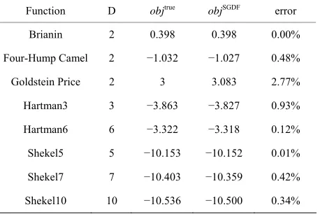
We use eight test functions [28]: Brianin, Six-Hump, Goldstein Price, Hartman3, Hartman6, Shekel5, Shekel7, and Shekel10. These functions have known optimal val-ues and optimal solutions, and have been used widely for testing purpose in research papers. For these functions, their dimensions and known optimal values are tabulated

in the Table 1. We also show the optimal values from SGDF side-by-side with the true optimal value in Table 1, which clearly shows that SGDF is capable of achiev-ing high accurate results.

Table 2 shows number of failures for each algorithm as a measure of accuracy. SGDF has no failure, which is also achieved by MS. All other algorithms have difficulty for high dimensional problems. Especially the genetic algorithm and pattern search without polling option ex-hibit high failure rates.The multi-start strategy (MS), though simple, works very well. SGDF, on the other hand, uses a more complicated strategy. It uses global information of the objective function in the global prob-ing phase, and generates searchprob-ing directions pointprob-ing to region with high objective values on average. This searching heuristics is fundamentally different from the local searching idea. Apparently, this innovative search-ing heuristics can also be coupled with the simple multi- start idea to enhance its success rate. However, multi- start inherently increases the computation effort as seen in the next table. Hence how to efficiently combine strength from both methods is a subject of future re-search.

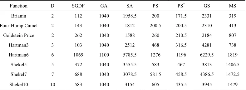
[image:8.595.310.539.581.734.2]

Table 3 shows the median number of function calls used by each algorithm as a measure of efficiency. It is clear that SGDF uses much less function calls than multi- start algorithm. A further calculation shows that SGDF uses 65% less function calls than multi-start algorithm. This is not a surprise since multi-start algorithm runs from ten starting points so as to increase its chance of hitting the global. Global Search also uses multiple start-ing points, but it drops those unpromisstart-ing ones sooner. However, Global Search does not simply run local solver from each starting point, it has a more complicated strategies including basin radius estimation, two stage search, and dynamic threshold, etc, which increases its function calls significantly. Pattern Search with addi-tional searching option is more efficient than Pattern Table 1. Compare the true and SGDF optimal objective values.

Function D objtrue objSGDF error

Brianin 2 0.398 0.398 0.00%

Four-Hump Camel 2 −1.032 −1.027 0.48% Goldstein Price 2 3 3.083 2.77%

Hartman3 3 −3.863 −3.827 0.93%

Hartman6 6 −3.322 −3.318 0.12%

Shekel5 5 −10.153 −10.152 0.01% Shekel7 7 −10.403 −10.359 0.42% Shekel10 10 −10.536 −10.500 0.34%

Table 2. Median number of failures.

Function D SGDF GA SA PS PS* _{GS MS}

Brianin 2 0 0 0 0 0 0 0

Four-Hump Camel 2 0 0 0 1 0 0 0

Goldstein Price 2 0 11 0 0 8 0 0

Hartman3 3 0 1 0 11 7 0 0

Hartman6 6 0 0 0 0 0 0 0

Shekel5 5 0 26 9 23 17 0 0

Shekel7 7 0 26 10 23 19 5 0

Shekel10 10 0 26 13 22 21 1 0

SGDF: sparse grid derivative free; GA: genetic; SA: simulated annealing; PS: pattern search (direct search); PS*_{: pattern search with}

[image:9.595.103.497.295.439.2]

polling option on; GS: global search; MS: multi-start.

Table 3. Median number of function calls.

Function D SGDF GA SA PS PS* _{GS MS}

Brianin 2 112 1040 1958.5 200 171.5 2331 319

Four-Hump Camel 2 143 1040 1812 200.5 200.5 2310 413

Goldstein Price 2 262 1040 1588 260 210.5 2184 807

Hartman3 3 103 1040 2512 468 316.5 4281 738

Hartman6 6 1069 1100 5785.5 1276 1196 6229.5 1819

Shekel5 5 372 1040 3555.5 583 467 3813 1406.5

Shekel7 7 688 1040 3078.5 581.5 458.5 4386.5 1472.5

Shekel10 10 583 1040 3154 605 435.5 3945 1479

SGDF: sparse grid derivative free; GA: genetic; SA: simulated annealing; PS: pattern search (direct search); PS*_{: pattern search with}

polling option on; GS: global search; MS: multi-start.

Search with polling step only. Simulated Annealing and Genetic algorithms apparently use more function calls.

Tables 2 and 3 together show that SGDF is both ac-curate and efficient. Multi-start is acac-curate but slightly more expensive. Global Search and Simulated Annealing could be accurate at the expense of more than ten times function calls as SGDF. The Pattern Search with or without searching step is efficient, but could generate a solution far away from optimum if started randomly. Genetic algorithm has reported success for more compli-cated biological system optimization but does not advan-tage in this experiment.

It appears that the starting point strategy of SGDF is effective. By using a single starting point, i.e., the global center of gravity, SGDF is able to find solutions very close to a global optimum for eight testing problems. In the contrast, other algorithms use random starting points have more or less fails, except for multi-start algorithm. The multi-start algorithm uses ten starting points in each of the twenty six runs. It is interesting to observe that for this experiment there is always one good starting point out of the ten.

7. Conclusions and Discussion

derivative free optimization methods, including Pattern Search, Global Search, Multi-start, Simulated Annealing and Genetic algorithms, is favorable.

The new algorithm is intended to solve practical prob-lems, where derivative information is not available and function evaluation is expensive. For these problems, priority is given to generate a high quality near-optimal solutions within computing budget. On the other hand, we realize that many of these problems also involve in-teger decision variables, which is not handled by the current algorithm, hence it is a topic for our future re-search.

REFERENCES

[1] J. D. Pinter, “Global Optimization in Action,” Kluwer, Dordrecht, 1996. doi:10.1007/978-1-4757-2502-5

[2] A. J. Booker, J. E. Dennis Jr., P. D. Frank, D. W. Moore and D. B. Serafini, “Managing Surrogate Objectives to Optimize a Helicopter Rotor Design: Further Experi- ments,” Proceedings of 8th AIAA/ISSMO Symposium on Multidisciplinary Analysis and Optimization, St. Louis,

1998.

[3] C. Audet and D. Orban, “Finding Optimal Algorithmic Parameters Using Derivative-Free Optimization,” SIAM Journal on Optimization, Vol. 17, No. 3, 2006, pp. 642-

664.

[4] R. Oeuvary and M. Bierlaire, “A New Derivative-Free Algorithm for the Medical Image Registration Problem,”

International Journal of Modelling and Simulation, Vol.

27, No. 2, 2007, pp. 115-124.

[5] T. Levina, Y. Levin, J. Mcgill and M. Nediak, “Dynamic Pricing with Online Learning and Strategic Consumers: An Application of the Aggregation Algorithm,” Opera- tions Research, Vol. 57, No. 2, 2009, pp. 327-341.

[6] P. Mugunthan, C. A. Showmaker and R. G. Regis, “Com- parison of Function Approximation, Heuristic and Deri- vative-Based Methods for Automatic Calibration of Com- putationally Expensive Groundwater Bioremediation Mod- els,” Water Resources, Vol. 41, 2005.

[7] J. A. Neldder and R. Mead, “A Simplex Method for Fun- ction Minimization,” TheComputer Journal, Vol. 7, No.

4, 1965, pp. 308-313. doi:10.1093/comjnl/7.4.308

[8] C. Audet and J. E. dennis Jr., “Analysis of Generalized Pattern Searches,” SIAM Journal on Optimization, Vol.

13, No. 3, 2003, pp. 889-903.

doi:10.1137/S1052623400378742

[9] T. G. Kolda, R. M. Lewis and V. Torczon, “Optimization by Direct Search: New Perspectives on Some Classical and Modern Methods,” SIAM Review, Vol. 45, No. 3, 2003,

pp. 385-482. doi:10.1137/S003614450242889

[10] T. A. Winslow, R. J. Trew, P. Gilmore and C. T. Kelley. “Doping Profiles for Optimum Class B Performance of GaAs MESFET Amplifiers,” Proceedings of the IEEE/ Cornell Conference on Advanced Concepts in High Speed Devices and Circuits, Ithaca, 5-7 August 1991, pp. 188-

197.

[11] A. R. Conn, K. Scheinberg and P. L. Toint, “On the Con- vergence of Derivative-Free Methods for Unconstrained Optimization,” Approximation Theory and Optimization: Tributes to M. J. D. Powell, Cambridge University Press, Cambridge, 1997, pp. 83-108.

[12] M. J. D. Powell, “The NEWUOA Software for Uncon- strained Optimization without Derivatives,” Technical Report, DAMTP 2004/NA08, Department of Applied Ma- thematics and Theoretical Physics, University of Cam- bridge, Cambridge, 2004.

[13] M. Marazzi and J. Nocedal, “Wedge Trust Region Meth- ods for Derivative Free Optimization,” Mathematical Pro- gramming, Vol. 91, No. 2, 2002, pp. 289-305.

doi:10.1007/s101070100264

[14] A. R. Conn, K. Scheinberg and L. N. Vicent, “Introduc- tion to Derivative-Free Optimization,” MOS-SIAM Se- ries on Optimization, SIAM, Philadelphia, 2009.

doi:10.1137/1.9780898718768

[15] C. Audet and J. E. Dennis Jr., “Mesh Adaptive Direct Search Algorithms for Constrained Optimization,” SIAM Journal on Optimization, Vol. 17, No. 1, 2006, pp. 188-

217. doi:10.1137/040603371

[16] D. Jones, C. Perttunen and B. Stuckman, “Lipschitzian Optimization without the Lipschitz Constant,” Journal of Optimization Theory Applications, Vol. 79, No. 1, 1993, pp. 157-181, doi:10.1007/BF00941892

[17] W. Huyer and A. Neumaier, “Global Optimization by Multileve Coordinate Search,” Journal of Global Opti- mization, Vol. 14, No. 4, 1999, pp. 331-355.

doi:10.1023/A:1008382309369

[18] X. Wang, D. Liang, X. Feng and L. Ye, “A Derivative- Free Optimization Algorithm Based on Conditional Mo- ments,” Journal of Mathematical Analysis and Applica- tions, Vol. 331, No. 2, 2006, pp. 1337-1360.

[19] G. W. Wasilkowsi and H. Wozniakowski, “Explicit Cost Bounds of Algorithms for Multivariate Tensor Product problems,” Journal of Complexity, Vol. 11, No. 1, 1995, pp. 1-56. doi:10.1006/jcom.1995.1001

[20] M. S. Bazarra, H. D. Sherali and C. M. Shetty, “Nonlin- ear Programming: Theory and Algorithms,” 3rd Edition, Wiley, John & Sons, Hoboken, 2006.

[21] H.-J. Bungartz and M. Griebel, “Sparse Grids,” Acta Nu- merica, Vol. 13, 2004, pp. 147-269.

[22] T. Gerstner and M. Griebel, “Numerical Integration Using Sparse Grid,” Numerical Algorithms, Vol. 18, 1998, pp.

209-232.

[23] F.-J. Delvos, “D-Variate Boolean Interpolation,” Journal of Approximation Theory, Vol. 34, No. 2, 1982, pp. 99-

114. doi:10.1016/0021-9045(82)90085-5

[24] A. R. Conn, N. I. M. Gould and P. L. Toint, “Trust-Re- gion Methods,” MOS-SIAM Series on Optimization,SIAM,

Philadelphia, 2000. doi:10.1137/1.9780898719857

[25] Z. Ugray, L. Lasdon, J. Plummer, F. Glover, J. Kelly and R. Marti, “Scatter Search and Local NLP Solvers: A Mul- tistart Framework for Global Optimization,” INFORMS Journal on Computing, Vol. 19, No. 3, 2007, pp. 328-340.

doi:10.1287/ijoc.1060.0175

linking,” In: J.-K. Hao, E. Lutton, E. Ronald, M. Schoe- nauer and D.Snyers, Eds., Artificial Intelligence, Springer, Berlin, Heidelberg, 1998, pp. 13-54.

[27] D. E. Goldberg, “Genetic Algorithms in Search,” Opti- mization & Machine Learning, Addison-Wesley, Boston,

1989.