http://www.scirp.org/journal/ajor ISSN Online: 2160-8849
ISSN Print: 2160-8830
MIP Formulations and Metaheuristics for
Multi-Item Capacitated Lot-Sizing Problem with
Non-Customer Specific Production Time
Windows and Setup Times
Ridha Erromdhani
1*, Abdelwaheb Rebaï
21Department of Quantitative Methods and Information Technology, Faculty of Economic and Management, Sfax, Tunisia 2Department of Quantitative Methods, Faculty of Economic and Management, Sfax, Tunisia
Abstract
Our research focuses on the development of two cooperative approaches for resolution of the multi-item capacitated lot-sizing problems with time win-dows and setup times (MICLSP-TW-ST). In this paper we combine variable neighborhood search and accurate mixed integer programming (VNS-MIP) to solve MICLSP-TW-ST. It concerns so a particularly important and difficult problem in production planning. This problem is NP-hard in the strong sense. Moreover, it is very difficult to solve with an exact method; it is for that reason we have made use of the approximate methods. We improved the variable neighborhood search (VNS) algorithm, which is efficient for solving hard com-binatorial optimization problems. This problem can be viewed as an optimi-zation problem with mixed variables (binary variables and real variables). The new VNS algorithm was tested against 540 benchmark problems. The perfor-mance of most of our approaches was satisfactory and performed better than the algorithms already proposed in the literature.
Keywords
Variable Neighborhood Decomposition Search, Formatting, Metaheuristics, Production Planning, Capacitated Lot Sizing, Mixed Integer
Programming, Matheuristics, Production Time Windows
1. Introduction and Motivations
The multi-item capacitated lot-sizing problem with time windows and setup times (MICLSP-TW-ST) has been an important part of material requirement planning (MRP) system. This problem is both complex and very important.
How to cite this paper: Erromdhani, R. and Rebaï, A. (2017) MIP Formulations and Metaheuristics for Multi-Item Capacitated Lot-Sizing Problem with Non-Customer Specific Production Time Windows and Setup Times. American Journal of Opera-tions Research, 7, 83-98.
https://doi.org/10.4236/ajor.2017.72006 Received: January 12, 2017
Accepted: March 11, 2017 Published: March 14, 2017 Copyright © 2017 by authors and Scientific Research Publishing Inc. This work is licensed under the Creative Commons Attribution International License (CC BY 4.0).
http://creativecommons.org/licenses/by/4.0/
Wherein, we seek to minimize the total cost of production, preparation and in-ventory. It comes to determine a production plan of a set of N products, for a time horizon consisting of T periods. This plan is finite capacity and must con-sider a set of additional constraints. Indeed, the manufacture of a unit of product
i to the period t engenders a production cost pit and requires a manufacture time of tfi units of the capacity of the resource (Ct). The cost of preparation cprit is generated at each period. A storage cost of a unit of the product i at the end of period t is hit. All these costs are deterministic. Each request must be pro-duced before a deadline Di and of the same it becomes even available at a pe-riod ri “availability period” before which she cannot be produced.
The decision variables are Xit which represents the product quantity i manufactured in the period t and Yit, the preparation variable that is equals 1 if Xit >0. We need also to define Yit as a binary variable equal to 1 if item i is produced at period t and 0 otherwise (i.e. if Xit > 0 only if Yit = 1).
•For this problem we dispose a set of command during a time horizons con-sisting of T periods in seek to satisfy the customer following delays taking into account the capacity constraint and fixed charge and variable launch of each product. Several extensions have been presented for this problem. We can there-fore, classify those problems of the lot sizing at a level by Kuik and Solmon [1]
and several production levels by Brahimi et al.[2]. Similarly, for the problem at a single level, they can be classified into problems to several products or to a single product. Several extensions have been proposed, and one finds the problem of several products with the re-fabrication (Richter and Sonbrutzki [3]), preparation time (Trigeiro et al. [4]), and with common preparations (Suerie and Stadtler
[5]). One finds these same extensions with the problems to a single product, in particular the case without capacity (Wagner and Whitin [6]), and the products of re-fabrication (Golany, Yan, and Yu [7]). One also finds the case with time win-dows on the demand (Lee, Cetinkaya, and Wagelmans [8]). It has always been considered that the requests can be prepared early in the planning horizon.
However, there are several constraints that do than this hypothesis is not true. This is the case, for example, when the raw material is supplied to us at different pe-riods. That is why we made recourse to the time window constraint and its impor-tance in modeling and solving production planning problems, and in this case one should consider for each request an availability date in addition to her delivery date. In the particular case with time windows for non-specific customers, products arriving at a period s are used to satisfy the demands for which the due period expired is t (s≤t) and which are not yet covered by products arriving before (First-In-First-Out).
The time window constraint signifies that there is a time interval where the customer demand can be satisfied without inventory and backlogging costs. Under this constraint, two cases may be presented: The specific customer case means that each specific demand should be satisfied within a given time interval. Therefore, the production between two periods’ t1 and t2 can only satisfy the
specific demand available before t2. On the other hand, the non-specific
windows (s t1;1) and (s t2;2), it holds that s1≤s2 and t1≤t2.
In the literature, Dauzère-Pérès et al.[9] are the first ones who presented the production time windows constraint in the LSP context. They have treated the customer specific case with single item. Wosley [10] considered the LSP with time windows under non-specific customer case. The LSP with non customer specific model is equivalent to the single item problem with stock upper bounds by Wosley [10], whereas, in other study, Van den Heuvel and Wagelmans [11]
have showed that this model is equivalent to the lot-sizing model with a rema-nufacturing option and the lot-sizing model with cumulative capacities.
In the literature, the first exact algorithm was presented by Wagner & Whitin
[6] denoted (WW), is polynomial (initially resolved in O (T2)). It’s of a dynamic
programming algorithm which explores the solution space of a problem for find the optimum. Recently, the complexity of dynamic algorithm of the lot sizing prob-lem at a product and without capacity constraints has been improved at O (TlogT). Pochet & Wolsey [12], there are also several variations of the basic problem: the stock shortage, the preparation time and refabrication. For states of the re-cent art on the problem (see Brahimi & Nordli [2]). Karimi et al. [13] and Dauzère-Pérès & Nordli [9] have proven that the algorithmic complexity for the lot sizing problem to a product as well as without capacity constraint with non- customer specific is NP-complete.
Lee & Wagelmans [8] imposed some assumptions on costs and have studied two cases: with and without the out of stock. For the case, with no stock shortage, an algorithm in O (T2) time has been proposed. When stock shortage is
permit-ted the problem is solved in O (T3) time.
Our particular contribution relative to this subject is the introduction of a new model with constraints of time window. For which, we have developed two algo-rithm based mainly on two new formulations mathematical and analysis of me-thods of solving several classes of problems.
The choice of this problematic has relied on the reasons following: First of all we will exploit nature of the problem for propose a new resolution approach based on decomposition. In the second place, this algorithm of metaheuristic has proven its performance in solving of mixed-variable optimization problems.
Finally, this algorithm has never been applied to resolve the problems of mul-ti-item capacitated lot-sizing problems with time windows and setup times.
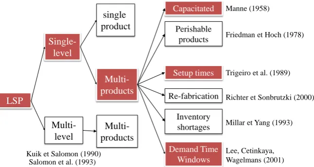
In our study, we have focused on the problems at one level but at several products under capacity constraint with time windows and setup times. Let LSP denotes the lot sizing problem, as is shown in Figure 1.
The remaining of the paper is organized as follows: Section 2 describes an MIP formulation of the MICLSP-TW-ST problem, computational experiments are described in Section 3, and the conclusions and future researches are presented in Section 4.
2. Mathematical Formulation and Resolution
Figure 1. Classification of lot sizing models (Based on illustrations by Brahimi et al. [17]).
products over a time horizon consisted of T periods. The objective is determined the periods of productions and the quantities to produce, in order to minimize the total production, setup and holding costs to satisfy all requests.
In this model, N and T stand for the number of items and the number of pe-riods in the planning horizon respectively. The following notations are used in order to describe the mathematical model of the MICLSP-TW-ST problem:
Parameters for the MICLSP-TW-ST
T Number of time periods.
N Number of products.
t Index of time periods. Where t=1T .
i Index of products. Where i=0 corresponds to the raw material and i=1N to the finished products.
it
d Demand for item i at period t.
it
p Unit production cost of finished product i in period t.
it
s Setup cost of finished product i in period t.
it
h Unit holding cost of finished product i in period t.
t
C Available capacity at period t.
ikt
d External demand for item i available at period k that should be produced before period t.
0 i
I Initial inventory of item i.
i
r Launching production of item iin period t requires a setup time i from the joint resource.
i
σ Requires units of the joint resource.
it D
represents the aggregate demand in period t, i.e.
1 t
it ikt k
D d
=
=
∑
.Without loss of generality we assume that each of the items 1, ,
i= N has a distinct time window.
LSP
Single-level
Multi-level
single product
Multi-products
Setup times
Perishable products
Capacitated
Re-fabrication
Inventory shortages
Demand Time Windows
Richter et Sonbrutzki (2000)
Millar et Yang (1993)
Lee, Cetinkaya, Wagelmans (2001) Trigeiro et al. (1989) Friedman et Hoch (1978) Manne (1958)
Kuik et Salomon (1990) Salomon et al. (1993)
The decision variables are as follows:
it
X is the quantity of product i prepared at period t.
it
I is the inventory level i at the end of period t and
it
Y a binary variable. Which takes the value 1 if there is a setup of i in
t and 0 otherwise (Xit >0 only if Yit =1).
• Model MICLSP-TW-ST
(
)
1 1
Min
N T
it it it it it it i t
s Y p X h I
= =
+ +
∑∑
(1)Subject to:
, 1 ,
i t it it it
I − +X −I =D ∀i t (2)
1 1
,
t t T
ik iks
k k s k
X d i t
= = =
≤ ∀
∑
∑∑
(3)(
)
2 2 2
1 1
1 2 1 2 , ,
t t t
ik ikl
k t k t l k
X d i t t t t
= = =
≥ ∀ ≤
∑
∑ ∑
(4)(
)
1
N
i it i it t i
X r Y C t
σ
=+ ≤ ∀
∑
(5), T
it il it
l t
X d Y i t
=
≤ ∀
∑
(6)}
{
0,1 ,it
Y ∈ ∀i t (7)
, 0 , it it
X I ≥ ∀i t (8)
The objective (1) is to minimize total setup, production and holding costs. Constraints (2) are the inventory balance equations. Constraints (3) state that the cumulative production in the first t periods does not exceed the cumulative quantity available from periods 1 to t. Constraints (4) guarantees that the con-straints of time windows are satisfied. This concon-straints warrant that the produc-tion which is to be performed between two periods t1 and t2.
The capacity constraints are represented by (5). Constraints (6) relate the bi-nary setup variables Yit to the continuous variables Xit. Finally, the integrality and non-negativity constraints are Constraints (7) and (8).
This problem may be seen as an optimization problem with variables mixed combined with binary variables and variable real.
2.1. Solving Multi-Item Capacitated Lot-Sizing Problems
mathemati-cal programming to determine the amounts of production and storage for each item during each period.
The general principle is to isolate the difficult part of the easy part of the problem and subsequently resolve the difficult part by an approached method and the easy part by an exact algorithm. We have developed two based algo-rithm principally on two new mathematical formulations to satisfy the capac-ity constraints.
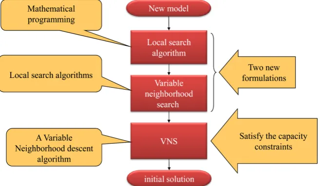
We propose a procedure approached based on local search for the improve-ment of that solution. After creating an initial solution (shown in Figure 2), a phase of improvement is introduced by performing movements in the prepa-ration sequence, because any changes in this sequence leads to a new solution (Y is a binary matrix). The vicinity of such a solution can be defined by the solution obtained in changing one or more components same time.
2.2. A Local Search Algorithm Based on Mathematical
Programming (Algorithm 1)
For the first algorithm we proposed solve the problem with binary variables using a local search algorithm that will allow us to generate solutions in two neighboring structures.
The first is to be introduced or reviewed eliminate one day of production whereas second will allow us to change a day of production by another.
Whenever a new solution is generated, a new mathematical program will take place taking into account the partial solution obtained by the local search method, which going to make being an exact resolution for the definition of quantities to be produced for each product during each period.
• A new mathematical formulation of the first algorithm
A new formulation of the MICLSP-TW-ST may be presented by a linear mixed integer program as follows:
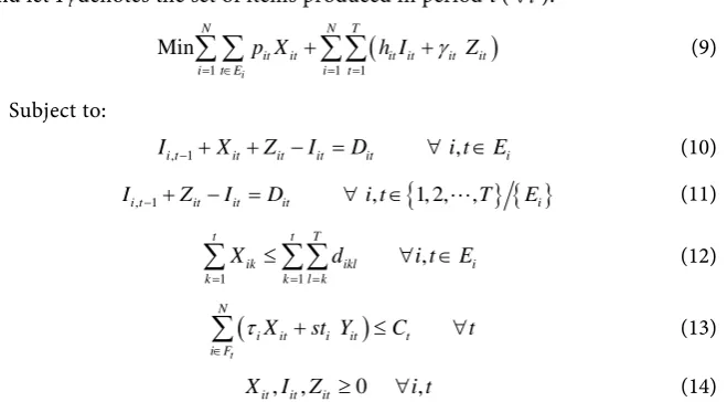
[image:6.595.211.540.524.715.2]Let Ei denotes the set of periods where yit takes the value of 1. (∀i)
and let Ft denotes the set of items produced in period t (∀t).
(
)
1 1 1
Min
i
N N T
it it it it it it
i t E i t
p X h I γ Z
= ∈ = =
+ +
∑ ∑
∑∑
(9)Subject to:
, 1 ,
i t it it it it i
I − +X +Z −I =D ∀i t∈E (10)
}
{
{ }
, 1 , 1, 2, ,
i t it it it i
I − +Z −I =D ∀i t∈ T E (11)
1 1
,
t t T
ik ikl i
k k l k
X d i t E
= = =
≤ ∀ ∈
∑
∑∑
(12)(
)
t
N
i it i it t
i F
X st Y C t
τ
∈
+ ≤ ∀
∑
(13), , 0 ,
it it it
X I Z ≥ ∀i t (14)
In this new formulation, we introduced a new decision variable denoted
it
Z who means the quantity demand breaking than one item i at period t and γit is the cost associated with this variable. The new variable Zit, is used to create a feasible solution of the problem in order to calculate the value of the objective function. In addition, this new decision variable Zit meas-ures the distance between region admissible and inadmissible of the search space. Indeed, the acceptance of a non-feasible solution will be penalized by a very high cost γit.
According to basic math, this problem is a problem in whole numbers, in-cluding binary variables such as the configuration of each item for each pe-riod and continuous variables such as production quantities and stocks.
The complexity of the problem increases according to the numbers of items. In addition the size of the neighborhood is very wide which leads excessive execution times. We propose a procedure approach based on local search for improving this solution.
After you create an initial solution, a phase of improvement is introduced by performing movements in the preparation sequence, because any changes in this sequence led to a new solution.
First of all, all the elements of the matrix Yit are initialized to 1 for all items and all periods and the mathematical program will be resolved. In the solution obtained, the quantities produced are determined. On the basis of this modification within the matrix Y, the problem will be reformulated and solved.
These stages will be repeated until there is no quantity Xit =0 which cor-responds to a preparation Yit different from zero. We used two structures of neighborhood to guide the local search to converge less rapidly to a local op-timum.
The first structure of used neighborhood is based on a single movement i.e. a single component of Y will be changed with every movement, as is shown in
[image:7.595.213.543.82.264.2]im-provements, if a local optimum was found, the second structure of neighbor-hood will be realized, as is shown in Figure 4.
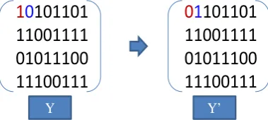
In this structure, the movement to base to two-segment is used. Two com-ponents will be changed. For each item i, for each period t, all possible move-ments of permutation are used. A permutation movement consists in permute the values of two distinct periods for only one items i in the matrix Y. This step will be repeated up the absence of possible improvements. The choice of the change of the structure of a single item instead of two items is based on an extensive experiment. This second neighborhood structure will allow us to change a day of production by another.
An every time a new solution is generated, a new mathematical program will take place by taking into account the partial solution obtained by the me-thod of local search. The algorithm will stop when the local optimum of the second procedure and the first procedure is the same.
2.3. Variable Neighborhood Search Based on a Local Search
Algorithm (AL2)
In order to reduce the computing time engendered by the resolution of the ma-thematical program, we have developed a second algorithm based on a decom-position scheme which consists in transforming the problem of a problem mul-ti-produced in a mono-produced problem; this procedure consists in consider-ing the production item by item. Every time one seeks to optimize the days of production of one item, we consider that the quantities to produce other prod-ucts during the horizon of time are fixed to the values of the best solution al-ready obtained.
[image:8.595.205.539.480.580.2]• New mathematical formulation of the second algorithm
Figure 3. The first procedure of local search (a single movement).
Figure 4. The second local search procedure (Two components will be changed).
10
0010
110010
010110
01
0010
110010
010110
11
0010
110010
010110
Elimination a day of production
Inserting a day of production
1
0
101101
11001111
01011100
11100111
0
1
101101
11001111
01011100
11100111
[image:8.595.279.469.618.703.2]Based on the results of AL1, it is shown that the phase of the resolution of the mathematical programming is relatively slow. Therefore, we have proposed a decomposition scheme of the problem for reducing its size i.e. the number of constraints and the number of variables.
For each item; after performing the move, we evaluate this move according to the single item LSP by considering the remaining items as fixed. So, the mul-ti-item LSP is transformed to the single-item LSP by performing the moves to the setup sequence of an item *
i and assuming that the setup sequence for all remaining items are known. Therefore, in each iteration, a new mathematical formulation of the problem is developed and solved:
(
)
(
) (
)
* 1
Min , ,
i
T
i i t i t i t i t i t
t E t
X I Z p X∗ ∗ h I∗ ∗ γ∗Z∗
∈ =
=
∑
+∑
+ (15)*, 1 * *
s.t. Ii t− +Xi t+Zi t∗ =Di t∗ +Ii t∗ t∈Ei , (16)
{
}
*, -1 1, 2, , i ,
i t i t i t i t
I∗ +Z∗ =D∗ +I∗ t∈ T E (17)
*
1 1
t t T
i k i kl i
K k l k
X∗ d∗ t E
= = =
≤ ∈
∑
∑∑
(18)' ' ' 1 1
'
1, 2, , ,
N N
t i i t
i i t i i t
i i
i i
X C Y X t T
δ
∗ ∗τ
∗ ∗δ
∗
∗
= =
≠
≤ −
∑
−∑
= (19)* * *,
T
i t i l i
l t
X D t E
=
≤ ∈
∑
(20)*, *, * 0 1, , t t i t i t
I X Z ≥ t= T (21)
where Ei* the set of periods whose Yit =1 * 1, 2,∀i = ,N,
The objective function (15) minimizes the total cost induced by the produc-tion plan that is producproduc-tion costs, inventory costs and penalty for the demand shortage costs for the item *i .
The constraints capacity (19) is modified while taking into account the known production of the items other than *i .
The evaluation of each move is computed according to the resolution of the mathematical programming presented above.
Indeed, if one reduces our mathematical program we will accelerate the reso-lution of the problem, it’s going to enable us to use a decomposition scheme which permutes from moving a local optimum and explore a larger region of the space search. The evaluation of motions with AL2 seems faster than that of AL1 since the reduction in the size of the mathematical program.
This second algorithm based on a decomposition scheme which consists in transforms the lot sizing problem multi products to a lot sizing problem to a fi-nite capacity to single product. Our idea is to propose a new procedure for im-provement using local search algorithm to variable neighborhood see Hansen
[14] and Mladenović [15].
Our idea is to propose a new improvement procedure by using the Iterated Local Search algorithm (ILS) proposed by Lourenço et al.[16].
This algorithm consists of two main steps: local search and perturbation. The first step leads to perform some moves to the current solution. The local optima found will be subject to the perturbation by applying random moves. These steps will be repeated until reaching a given stopping criterion.
The ILS algorithm has the advantage to explore regions far from the current region of the search space. So, once the best solution is found in a large region, it is necessary to go quite far to get better solutions. Therefore, this algorithm em-ploys the concept of perturbation to move from one region to another which can be more profitable.
In our application, the neighbourhood structures used here are also the same used in algorithm1. However, within the local search, the way of solution’s evaluation of each move is based on the decomposition scheme described above.
3. Computational Experiments
This section reports computational experiments that evaluate the effectiveness of our algorithms and evaluate the performances against the proposed algorithms in the literature of the CLSP with time windows and set up times.
Our algorithms are implemented in the C++ programming language. We use the callable Cplex 9.0 library to solve the MILP problems. Computational expe-riments were performed on an Intel Core 2 CPU 2.67 GHz PC with 3.25 GB RAM.
The data sets used in our experiments are generated by Brahimi et al. [17]. These instance problems are based on the data sets of Trigeiro et al.[4] and ex-tended by adding the time windows. More detailed information about these test problems is available in Brahimi et al.[17].
3.1. Data Sets
The data sets used in our experiments are generated by Brahimi et al.[17]. These instance problems are based on the data sets of Trigeiro et al.[4] and extended by adding the time windows. More detailed information about these test prob-lems is available in Brahimi et al.[18].
The comparison was conducted after classifying the instances into 13 classes. For a time horizon will fixed at T = 20 periods and three values are used for the number of products N: 10, 20 and 30 products. We compared our approaches to resolution and we proposed several policies research local and procedures for improvement.
zero.
The utilization rate of total capacity is 75%, 85% and 95%. The time between two successive orders (TBO) is 1, 2 and 4. The average value of setup times over all products is 11 and 43 capacity unit. Finally, the production cost pit is set to 0 for all products and all periods.
3.2. Experimental Results
The Competing approaches used in our comparative study are the approaches developed by Brahimi et al.[17]. The first approach designated by (LR) is a la-grangian relaxation based heuristic.
The second one is an exact mixed integer programming approach based on a new reformulation of the problem and solved with a commercial software and denoted (MIPX). The last one is a mixed integer approach based on the original formulation of the problem and denoted by (MIPB).
To perform different quality measures by calculating the distances between lower and upper bounds of the same solution approach and between upper bounds (lower bounds) of different approaches. The distance or gap between two values
a and b, where a ≥ b, is calculated as follows:
( )
Gap a b, 200 a b
a b
− = ×
+ (22)
The formula Gap
( )
a b, 200 a b a b− = ×
+ is used instead of
(Gap
( )
a b, 100 a b a−
= × ) which overestimates the gap and
(Gap
( )
a b, 100 a b b−
= × ) which underestimates it. This approach was used. For
example, by Millar and Yang [19] and Brahimi et al.[18].
In order to evaluate our results depending of the competing approaches of li-terature. We began our analysis by counting the number of feasible solutions found on the 540 tested problems.
Our first experiment, reported in Tables 1-4, involves running the Variable Neighborhood Search based on a local search algorithm approach for at most 500 iterations, stopping earlier if optimality is proven. The CPU time given to Lagrangian relaxation was at least 1 s longer than that required by AL2 (see columns 10 - 12 of Table 2).
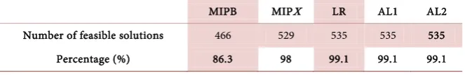
[image:11.595.208.540.684.738.2]As shown on Table 1. It can be seen that AL1 and AL2 are able to find 535 feasible solutions i.e. five instances remains unsolved as in LR algorithm.
Table 1. Number and percentage of problems for which feasible solutions were found (out of 540 problems).
MIPB MIPX LR AL1 AL2 Number of feasible solutions 466 529 535 535 535
Table 2. Average gaps and CPU times of the five solution approaches.
Parametre Value Gap (UB.LB) CPU (s)
MIPB MIPX LR AL1 AL2 MIPB MIPX LR AL1 AL2 10 16.58 2.92 2.76 3.79 2.02 3.32 3.33 2.0 3.38 2.05 N 20 24.01 1.32 1.02 1.37 1.08 5.79 5.81 4.14 5.14 4.66 30 25.64 1.26 0.58 1.64 0.50 7.84 7.95 5.92 5.09 5.36 75% 20.74 0.33 0.33 0.33 0.33 4.73 4.05 3.09 3.73 3.09 Capacity 85% 21.69 1.20 1.02 1.71 0.72 5.48 5.38 3.94 4.05 3.98 95% 23.89 4.14 3.15 4.16 2.68 6.73 7.66 5.12 7.64 5.34 1 2.32 0.60 0.70 0.84 0.73 4.16 3.36 2.69 4.16 3.14 TBO 2 21.39 1.01 0.90 172 0.95 6.25 6.09 4.55 5.48 4.26 4 52.15 4.06 2.88 3.96 1.94 6.54 7.64 4.90 5.36 4.90 CV 0.35 25.82 2.10 1.50 2.14 0.85 5.67 5.81 3.94 5.62 4.14 0.59 18.22 1.59 1.43 1.65 0.89 5.63 5.59 4.16 5.67 4.28 11 26.68 1.80 1.52 2.74 1.27 5.64 5.66 4.03 5.66 4.33 43 15.83 1.89 1.41 1.69 1.24 5.66 5.73 4.07 5.59 3.96 Global average 21.94 1.84 1.46 2.13 1.17 5.70 5.65 4.05 5.12 4.11
Table 3. Computational experiments of the proposed approaches.
Parameter Value
GAP UB (AL1. AL2) AL1 is better AL2 is better
gap gap
N
10 0.34 2.19 20 0.24 1.48 30 0.08 1.87
Capacity
75% 0.19 0.98 85% 0.31 1.37 95% 0.39 2.91
TBO
1 0.28 1.72 2 0.20 1.52 4 0.34 2.11
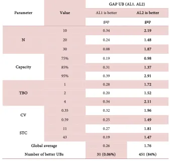
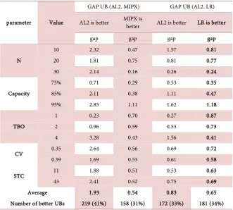
[image:12.595.202.541.419.739.2]Table 4. Gaps among UB (AL2), UB (MIPX) and UB (LR).
parameter Value
GAP UB (AL2. MIPX) GAP UB (AL2. LR) AL2 is better MIPX is better AL2 is better LR is better
gap gap gap gap
N
10 2.32 0.47 1.57 0.81 20 1.81 0.75 0.81 0.77 30 2.14 0.16 0.26 0.24
Capacity
75% 0.71 0.29 0.53 0.35 85% 2.11 0.38 1.11 0.47 95% 2.85 1.11 1.62 1.18
TBO
1 0.23 0.70 0.27 0.87 2 0.96 0.59 0.53 0.73 4 3.28 0.43 1.56 0.41 CV 0.35 2.64 0.56 0.69 0.72 0.59 1.69 0.53 0.61 0.58 STC 11 1.88 0.51 0.53 0.63 43 2.41 0.52 0.75 0.69 Average 1.93 0.54 0.83 0.65 Number of better UBs 219 (41%) 158 (31%) 172 (33%) 181 (34%)
The Lagrangian heuristic finds feasible solutions for most problems (99.1%).
i.e. 5 problems were unsolved. In addition, to these 5 problems, the MIPX ap-proach didn’t solve 6 more problems (feasible solutions were found for 98% of problems). Finally, the MIPB approach found feasible solutions for only 86.3% of the problems.
Table 2 summarizes the average gaps between upper bounds and lower bounds of each solution approach (columns 3 - 7) and the corresponding CPU times (columns 8 - 12). We note that these gaps are computed according to the feasible solutions provided by each approach. The best gaps are shown in bold-face.
The first observation is that the MIPB approach always generates larger gaps (21.94% on average) than the four other approaches. It can be seen that the AL2 have provided the best gaps in average for 10 classes of instances among 13 whereas the LR algorithm have provided 2 best gaps.
The last line of Table 2 also shows that the average gaps of MIPX, LR, AL1 and AL2 are 1.84%, 1.46%, 2.13% and 1.17%, respectively. AL2 outperforms all the other approaches with 1. 17%. Concerning our proposed approaches, we no-tice that AL2 is the best algorithm.
better (larger).
From Table 2, we can notice that the CPU time for the approaches in each class of instances. We can see that AL2 has the smallest CPU time (4.11) ac-cording to AL1, MIPB and MIPX. This is due to the decomposion scheme used in this algorithm, where, at each iteration, a single item problem is solved. On the other hand, the AL1 algorithm appears to be the slowest algorithm. Besides, the CPU time and the gaps of the proposed algorithms increase when the num-ber of items and TBO increase, and when the capacity is tightly constrained. In comparison with Brahimi et al.[17] approaches, the average CPU time values of our algorithms are relatively higher.
Table 3 shows the comparative study between the two proposed approaches in our paper. We compare the gap between the upper bound values provided by AL1 and AL2 according to Equation (22). It can be seen that AL2 is better than AL1 both in terms of average percentage deviations (0.26% in favour of AL1 and 1.76% in favour of AL2) and the number of better values of upper bounds. When AL2 is better than AL1, we find that the number of better upper bounds is large than the opposite case (31 upper bounds in favour of AL1 and 451 in favour of AL2). This is proving the contribution of the decomposition scheme introduced in AL2 for improving the results. However, in some cases AL1 is better than AL2 because AL1 explores more the depth of the space search.
Table 4 provides a comparative study between the upper bounds of AL2, MIPX and LR. It is shown that the proposed algorithm outperforms the two compared approaches. In average, for all classes, the percentage gap between AL2 and MIPX is equal 1.93% where AL2 is better than MIPX and is equal to 0.54% in the opposite case. The number of better upper bounds in favour of AL2 according to MIPX algorithm is 219. Regarding the LR algorithm, we see that AL2 is better in terms of average percentage deviations whereas the former is better in terms of number of improved upper bounds. However, as shown on
Table 4, the LR upper bounds were better than those of AL2 in 34% of the prob-lems and the bounds UB (AL2) were better for 33% of the test probprob-lems.
4. Conclusions
In our work, two cooperative approaches were proposed for solving multi-item capacitated lot-sizing problem with time windows and setup times where the non-customer specific demand is considered.
The problem is decomposed into two sub-problems: binary variables problem and continuous variables problem. Based on the complexity of each one of them, an exact approach using the mathematical programming is proposed for solving the problem with binary variables. On the other hand, the variable neighbor-hood search based on a local search algorithm, when applied to our efficient re-formulations quickly finds good lower bounds and takes longer time to find and improve feasible solutions. However, its steady state is reached after almost 2 h thus yielding better results if it is given “enough” time.
a local search algorithm quickly finds good feasible solutions. The comparative study is performed according to the representative approaches of the literature. The results have shown the efficiency of the proposed approaches.
References
[1] Kuik, R. and Salomon, M. (1990) Multi-Level Lot-Sizing Problem. Evaluation of a Simulated Annealing Heuristic. European Journal of Operational Research, 45, 25- 37. https://hdl.handle.net/11245/1.431251
https://doi.org/10.1016/0377-2217(90)90153-3
[2] Brahimi, N., Dauzère-Pérès, S., Najid, N. and Nordli, A. (2003) Alagrangian Relaxa-tion Heuristic for the Capacitated Single Item Lot Sizing Problem with Time Win-dows. 6th Workshop on Models and Algorithms for Planning and Scheduling Prob-lems, Aussois, 30 March-4 April 2003, 105-106.
[3] Richter, K. and Sombrutzki, M. (2000) Remanufacturing Planning for the Reverse Wagner/Whitin Models. European Journal of Operational Research, 121, 304-315. http://www.sciencedirect.com/science/article/pii/S0377-2217(99)00219-2
https://doi.org/10.1016/S0377-2217(99)00219-2
[4] Trigeiro, W., Thomas, L.J. and McLain, J.O. (1989) Capacitated Lot-Sizing with Se-tup Times. Management Science, 35, 353-366.
https://doi.org/10.1287/mnsc.35.3.353
[5] Suerie, C. and Stadtler, H. (2003) The Capacitated Lot-Sizing Problem with Linked Lot Sizes. Management Science, 49, 1039-1054.
https://doi.org/10.1287/mnsc.49.8.1039.16406
[6] Wagner, H.M. and Whitin, T.M. (1958) A Dynamic Version of the Economic Lot Size Model. Management Science, 5, 89-96. https://doi.org/10.1287/mnsc.5.1.89 [7] Golany, B., Yang, J. and Yu, G. (2001) Economic Lot-Sizing with Remanufacturing
Options. IIE Transactions, 33, 995-1003. https://doi.org/10.1080/07408170108936890
[8] Lee, C.Y., Cetinkaya, S. and Wagelmans, A.P.M. (2001) A Dynamic Lot-Sizing Model with Demand Time Windows. Management Science, 47, 1384-1395. http://www.jstor.org/stable/822493
https://doi.org/10.1287/mnsc.47.10.1384
[9] Dauzère-Pérès, S., Brahimi, N., Najid, N. and Nordli, A. (2002) The Single-Item Lot Sizing Problem with Time Windows. Technical Report, 02/4/AUTO, Ecole des Mines de Nantes, France.
[10] Wolsey, L.A. (2006) Lot-Sizing with Production and Delivery Time Windows. Ma-thematical Programming, 107, 471-489.
http://link.springer.com/article/10.1007%2Fs10107-005-0675-3 https://doi.org/10.1007/s10107-005-0675-3
[11] Van den Heuvel, W. and Wagelmans, A. (2008) Four Equivalent Lot-Sizing Models.
Operations Research Letters, 36, 465-470. https://doi.org/10.1016/j.orl.2007.12.003 [12] Pochet, Y. and Wolsey, L.A. (1994) Polyhedral for Lot-Sizing with Wagner-Whitin
Costs. Mathematical Programming, 67, 297-323. https://doi.org/10.1007/BF01582225
[13] Karimi, B., FatemiGhomi, S.M.T. and Wilson, J.M. (2003) The Capacitated Lot Siz-ing Problem: A Review of Models and Algorithms. Omega, 31, 365-378.
https://doi.org/10.1016/S0305-0483(03)00059-8
and Applications. European Journal of Operational Research, 130, 449-467. http://dblp.uni-trier.de/db/journals/eor/eor130.html#HansenM01
https://doi.org/10.1016/S0377-2217(00)00100-4
[15] Mladenović, N. and Hansen, P. (1997) Variable Neighborhood Search, Computers and Operations Research, 24, 1097-1100.
https://doi.org/10.1016/S0305-0548(97)00031-2
[16] Lourenço, H.R., Martin, O.C. and Stützle, T. (2002) Iterated Local Search. In: Glover, F. and Kochenberger, G., Eds., Handbook of Metaheuristics, Kluwer, Boston, 321- 353. https://arxiv.org/abs/math/0102188v1
[17] NadjibBrahimi, N., Dauzère-Pérès, S. and Wolsey, L.A. (2010) Polyhedral and La-grangian Approaches for Lot Sizing with Production Time Windows and Setup Times. Computers & Operations Research, 37, 182-188.
https://doi.org/10.1016/j.cor.2009.04.005
[18] Brahimi, N., Dauzère-Pérès, S., Najid, N. and Nordli, A. (2006) Single Item Lot Siz-ing Problems. European Journal of Operational Research, 168, 1-16.
http://www.sciencedirect.com/science/article/pii/S0377-2217(04)00392-3 https://doi.org/10.1016/j.ejor.2004.01.054
[19] Millar, H.H. and Yang, M. (1994) Lagrangian Heuristics for the Capacitated Mul-ti-Item Lot-Sizing Problem with Backordering. International Journal of Production Economics, 34, 1-15. https://doi.org/10.1016/0925-5273(94)90042-6
http://www.sciencedirect.com/science/article/pii/0925-5273(94)90042-6
Submit or recommend next manuscript to SCIRP and we will provide best service for you:
Accepting pre-submission inquiries through Email, Facebook, LinkedIn, Twitter, etc. A wide selection of journals (inclusive of 9 subjects, more than 200 journals)
Providing 24-hour high-quality service User-friendly online submission system Fair and swift peer-review system
Efficient typesetting and proofreading procedure
Display of the result of downloads and visits, as well as the number of cited articles Maximum dissemination of your research work
Submit your manuscript at: http://papersubmission.scirp.org/