Examining measures of the equilibrium Real Exchange Rate: Macroeconomic Balance and the Natural Real Exchange Rate Approaches

(1)

Munich Personal RePEc Archive

Examining measures of the equilibrium

Real Exchange Rate: Macroeconomic

Balance and the Natural Real Exchange

Rate Approaches

Wright, Nicholas Anthony

Bank of Jamaica

August 2013

Online at

https://mpra.ub.uni-muenchen.de/61170/

(2)

1 | P a g e Examining Measures of the Equilibrium Real Exchange Rate:

Macroeconomic Balance and the Natural Real Exchange Rate Approaches

Nicholas A. Wright1

Intern

International Economics Department

Research and Economic Programming Division

Bank of Jamaica

2013

Abstract

This paper examines two measures of the equilibrium real exchange rate using the Macroeconomic Balance (MB) and the Natural Real Exchange Rate (NATREX) approaches. Unlike previous studies, this study controls for business cycle effects and the debt sustainability position of countries on the current account, while providing a more comprehensive measure of relative productivity. A longitudinal panel econometric technique is utilized on a set of countries from the Western Hemisphere. These countries operate a managed float exchange rate system; have similar output per capita and equivalent levels of openness. The findings suggest that there were several intervals of exchange rate misalignment for each country, including Jamaica, over the 1990-2010 study period. The exchange rate misalignment series was found to be stationary which is an indication that there is a long-run equilibrium mean and a constant variance for exchange rate misalignment. This long-run misalignment mean is assumed to be zero by economic theory. The Autoregressive Distributive Lag (ARDL) error correction model suggests that disequilibrium in the exchange rate is adjusted by 46.2 per cent each year and the half-life deviation formula suggests that a half of the deviation in the exchange rate is corrected after 1.1 years for each country in the panel.

JEL Classification: F14, F31, F32

Keywords: Macro-balance approach, NATREX, Current Account Misalignment, Real Effective Exchange Rates, Exchange Rate Misalignment, Trade.

1

(3)

2 | P a g e

This applies specifically to the managed float exchange rate regime which targets monetary aggregates in manipulating the exchange rate among other things. This includes countries such as Afghanistan, I.R. of Burundi, Gambia, The Georgia, Guinea, Haiti, Jamaica, Kenya, Madagascar, Moldova, Mozambique, Nigeria, Papua New, Guinea, São Tomé and Príncipe, Sudan, Tanzania and Uganda. See IMF (2008) source in the references section for further details of the exchange rate regime of countries.

3

(5)

4 | P a g e levied against the Purchasing Power Parity (PPP) approach. In conforming to the other studies

that have sought to evaluate the ERER, this study will model the equilibrium exchange rate using

a set of macroeconomic fundamentals. Both the MB and the NATREX approaches will be

utilized which is consistent with most of the literature. In utilizing the MB framework, the

statistically robust fundamentals will be included, as well as additional indicators that have not

been accounted for in the literature.4

Additionally, unlike previous studies conducted on the ERER using a panel framework, this

study will consist of a panel of countries that has similar levels of income, equivalent exchange

rate regimes and similar levels of openness. Consequently, this study can be considered to be

more homogenous than panels in previous studies of this nature and the estimated panel

parameters from this study are less likely to be biased by sample selection. Finally, this study

seeks to expand the way in which some of the variables included in previous studies have been

measured. The NATREX approach will then be calculated using a reduced form equation using

the ARDL cointegration approach. The countries included in this study were the Dominican

Republic, Jamaica, Peru and Uruguay.5

The next section of this paper will provide a brief summary of the economic performance of the

countries analyzed. This is followed by a comprehensive review of the related findings from

previous studies that have estimated the ERER and the NATREX in Section 3. Section 4 reviews

the major statistical assumptions and procedures required for analyzing panel data. It also

delineates the models to be utilized in estimating the desired exchange rates and summarizes the

stationarity position of the variables to be used. Section 5 gives a presentation of the main

findings of the study and provides robustness tests to improve the reliability and validity of the

findings. The main conclusions and policy implications of the study are then discussed in Section

6.

2. Stylized Facts

Trade openness has facilitated global investment, with exchange rates being particularly

important to the growth and stability of a country‟s economy. The currencies of small open economies such as those included in the sample are usually more susceptible to domestic and

4

These include indicators such as recessionary periods and sustainable debt level dummies.

5

(6)

5 | P a g e global shocks. As a result, policymakers need to monitor movements in these countries exchange

rate to ensure price stability and internal and external balance. A brief outline of the trends in the

respective country‟s Real Effective Exchange Rate (REER), exports and current account balance is outlined below.6

2.1Case Study I: Jamaica

Annual data for Jamaica show that the value of Jamaican Dollar relative to the United States

dollar has steadily depreciated over the period 1990 – 2010. On a nominal basis, the Dollar lost approximately 15 per cent on average yearly, while the real exchange rate, as measured by the

REER, indicates an average appreciation of 3.2 per cent. In relation to the current account

balance, the trade balance being the largest component, deteriorated by 10.3 per cent per annum.

This was largely influenced by a 6.2 per cent increase in imports relative to a 2.1 per cent rise in

exports. In particular, fuel expenditure as a percentage of GDP has grown on average by 4.4 per

cent on an annual basis. This therefore contributed to a steady worsening in the current account,

averaging -10.5 per cent of GDP between 2000-2010, from an average of -2.8 per cent of GDP

between 1990-2000. These developments have led to a general loss in external competitiveness,

albeit partly offset by the impact of significant nominal depreciations in 2003 and 2008 (see

Figure 3, Appendix).

2.2 Case Study II: Peru

Peru has had a relatively stable economy over the past decade. This stability is mirrored through

a relatively small current account deficit over the last decade despite a world economic recession

in 2008. The Peruvian current account balance has averaged -0.9 per cent on an annual basis

between 2000-2010 which has been underpinned by an upward trend in exports as a percentage

of GDP and relatively stable fuel expenditure as a percentage of GDP. Over the sample period,

the nominal Peruvian Nuevo sol has depreciated by an average 23.0 per cent per annum while

the REER has appreciated by 1.8 per cent on average on a yearly basis (see Figure 4,

Appendix).

2.3Case Study III: Dominican Republic

The Dominican Republic has experienced two economic crises in the last decade, namely a

banking crisis in 2003 and the world economic recession of 2008. This has undoubtedly

6

(7)

6 | P a g e influenced the stability of the economic parameters being examined. The data show that the

country‟s exports, its current account balance to GDP ratio, the REER and the fuel expenditure as a percentage of GDP depicted relative stability prior to 2002 (see Figure 5, Appendix).

However, the impact of the banking crisis in 2003 led to strong structural changes in the banking

industry which further resulted in an improvement in the REER and the current account balance.

Prior to 2000 the current account balance had an average of -2.1 per cent which improved to a

surplus of 5.0 per cent during the 2003-2004 period. However, the global economic crisis in

2008 led to a reduction in exports and by extension a deterioration in the country‟s current account balance which averaged -7.8 per cent. Over the review period, the country‟s fuel averaged 10.2 per cent of GDP, which averaged 5.2 per cent between 1990 -2000 and 15.6 per

cent between 2000 -2010.

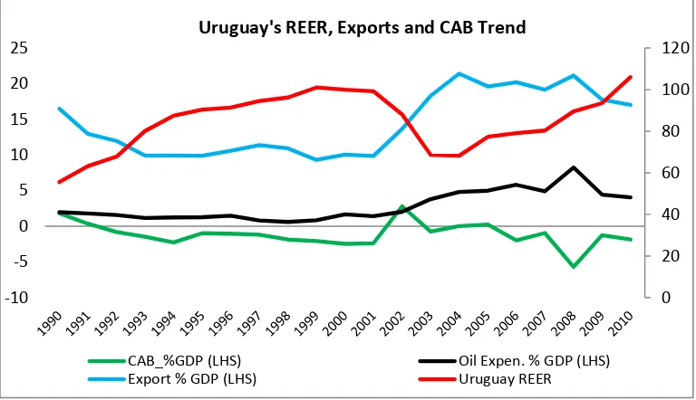
2. Case Study IV: Uruguay

Similar to the case of the Dominican Republic, Uruguay underwent two major economic crises

over the last decade. This includes a domestic banking crisis in 2001-02 and the global economic

recession in 2008. Following the domestic banking crisis, a significant depreciation of the

country‟s REER occurred which led to a subsequent increase in the country‟s exports. Over the three year period 2002-2004, the REER depreciated on average by 11.4 per cent per annum

while the export to GDP ratio grew by 29.9 per cent. The REER, however, appreciated during

the 2008-2010 recessionary period by 9.7 per cent while exports fell on average by 3.3 per cent.

Uruguay‟s fuel expenditure to GDP has averaged 4.2 per cent over the last decade. This has mirrored an average current account balance that was 0.7 per cent of GDP during the domestic

crisis period and -2.9 per cent of GDP during the international economic crisis period (see

Figure 6, Appendix).

3. Theoretical Review

In recent years, a myriad of studies have attempted to estimate the ERER utilizing varying

estimation procedures (such as the FEER, BEER, PEER and the NATREX) with various samples

that have vacillating levels of homogeneity. A large number of central banks in both developing

and developed countries have estimated the equilibrium exchange rate for their country. This has

(8)

7 | P a g e current account position and by extension its overall macroeconomic performance (Westaway

and Driver, 2004; Zalduendo, 2006, Eckstein and Friedman, 2011; Dunaway and Li, 2005;

MacDonald and Ricci, 2003 etc.). Eckstein and Friedman (2011) postulate that in a small open

economy, the real exchange rate has an important impact on countries growth trajectory and by

extension, their economic stability. They added that real exchange rate misalignments “could cause output loss and cyclical, inefficient allocation of resources, including low utilization of

factors of production”. Siregar and Rajan (2006) similarly argue that misalignment in the real exchange rate results in a country‟s loss of external competitiveness and growth reduction. In addition, they note that there is a possibility that sustained overvaluation could lead to a currency

crisis and sustained undervaluation could lead to overheating of the economy. It is also argued

that misalignment of the real exchange rate is responsible for global macroeconomic imbalances,

whereby countries with a grossly undervalued currency would automatically have an unfair

competitive advantage.

This theoretical review seeks to highlight the empirical studies that have sought to estimate the

equilibrium real exchange rate, placing emphasis on the importance of exchange rate

disequilibrium and highlighting the major limitations of previous studies. The main approaches

that will be focused on in this study are the macroeconomic balance approach and the natural real

exchange rate approach.

The seminal contributions to the MB approach of calculating the equilibrium real exchange rates

are owed to the IMF in the 1970s and 1980s (Isard et al, 2001) and the articulation of the FEER

approach by Williamson (1994). Isard et al (2001) notes that the MB approach makes

“quantitative assessments of exchange rates that are consistent with “appropriate” current account positions (external balance)” when economies are performing at potential output and stable prices (internal balance). One major criticism of the MB approach is that forecasting

using this model is highly unstable because of the uncertainty surrounding the forecasted

underlying current account and the assumptions made on the fundamentals moving forward.

Graham and Steenkamp (2012) argue that this can be addressed by providing a band for future

(9)

8 | P a g e In relation to the NATREX approach, Stein (1994) is the seminal contributor to its development.

This approach is conceptualized as the rate that would be actualized if unemployment was at its

natural level and speculative and cyclical market factors were removed (Siregar and Rajan,

2006). In a later paper, Stein (2001) articulates that the ERER is a sustainable rate that satisfies a

myriad of criteria. Among these criteria is the fact that at this rate, the economy is at full

capacity, which implies that actual output is equal to potential output, unemployment is at its

natural rate and inflationary adjustment is stable. In other words, internal balance is achieved.

Under the NATREX approach, Stein (2001) also posits that external balance must also be

achieved. This assumes that investors are indifferent between holding domestic and foreign

assets and there are neither upward nor downward pressures on the exchange rate. It also implies

that interest rates between the two countries converge to a stable mean and the country‟s debt obligations stabilize to a sustainable level.7

While the generally held consensus in the literature is that changes in the real exchange rate

(RER) influences the current account balance, Henry and Longmore (2003) found that the RER

does not play a significant role in determining Jamaica‟s current account. Against this background, they posit that the notion that the RER can be used as a tool for correcting the

unsustainability of the current account and improve competitiveness must be revisited for the

case of Jamaica and by extension other developing countries. On this basis, future studies ought

to examine the extent to which exchange rate misalignment in developing countries such as

Jamaica influences macroeconomic stability, especially where the current account has been

found to be unresponsive to changes in the RER.

4.0Methodological Framework

A panel analysis or longitudinal methodology was utilized which follows the same cross

sectional countries across time. The procedures are outlined in this section.

7

(10)

9 | P a g e 4.1Data Source and Sample Selection

Four countries were randomly selected from the group of countries located in the western

hemisphere, based on three selection criteria. The first criterion restricted the sample to countries

which utilized a managed float exchange rate regime. From this pool of countries, the remaining

criteria were applied. The second criterion utilized was the average income per capita, with an

aim of selecting countries with a similar economic landscape. Therefore, the countries included

in the sample were restricted to having average GDP per capita over the sample period that was

between US$2500 - $6500. Finally, the countries included in the sample had similar levels of

openness to the international market and largely underwent financial liberalization in the same

time period in their economic history. Consequently, the final sample had a moderate degree of

homogeneity.8 As mentioned in Section 1, the four countries which fit these criteria included the

Dominican Republic, Jamaica, Peru and Uruguay.

Annual data on these four countries were collected over a twenty-one (21) year time period

(1990-2010) and cumulatively formed a panel consisting of 84 observations. The data were

collected from a number of data sources and triangulated for accuracy and consistency. The

websites of the respective central banks were first consulted for the required data.9 However,

where the required data could not be garnered from these sources, the IMF international financial

statistics database, the World Economic Outlook (WEO) website, the World Bank database and

UNDATA were consulted to gather the required data.10 The sample clearly satisfies the central

limit theorem which suggests that if the other assumptions of the estimation techniques are met,

the estimates should be consistent.

4.2Econometric Models

4.2.1 The MB Approach

The MB approach to estimating the ERER has three steps as dictated by Isard et al (2001). This

approach is entrenched in the accounting identity which links a country‟s current account

8

Failure to satisfy the condition of randomization and failure to have homogenous entities in a panel framework may lead to issues of sample selection bias and lack of consistency in estimated coefficients.

9

Bank of Jamaica for Jamaica, Central Reserve Bank of Peru, Central Bank of Dominican Republic and the Banco Central del Uruguay (Central Bank of Uruguay).

10

(11)

10 | P a g e balance to the difference between domestic saving and domestic investment. The first step of the

process involves identifying each country‟s underlying current account position, which “is the

value of the current account that would emerge at prevailing exchange rates if all countries were

producing at their output levels and the lagged effect of past exchange rates changes had been

fully realized” (Isard, 2001).11

The second step of the process requires estimation of medium-run

equilibrium saving investment position. This is done by estimating an equilibrium relationship

between each country‟s current account balances and a set of fundamental determinants (Lee et al, 2006). The final step required in estimating the ERER is to compare the results from the first

two steps to determine the real exchange rate adjustment that would be necessary to close the gap

between the estimated underlying current account position and the medium-run equilibrium

saving investment position. This is done through evaluating the current account elasticity and by

evaluating how imports and exports respond to the changes in the real exchange rate.

 The Saving-Investment (S-I) Equilibrium(Current Account Norm)

While it is easy to attribute sustained current account deficits to the overvaluation of a country‟s

currency, it must be highlighted here that there are a number of intervening factors which may

influence the current account balance. These include the price elasticity of domestic demand for

foreign goods, the type of goods imported, the extent to which a country produces goods for

which it has a competitive advantage, the ease of doing business in the country and the country‟s

stage of development. Therefore, in modeling the current account as a function of non-price

fundamental factors, we are able to isolate the sustainable equilibrium current account balance

and the exchange rate which ensures this is achieved.

A plethora of fundamentals have been used in the literature to determine the medium-run S-I

equilibrium. Among the most robust variables are net foreign assets, fiscal balance, oil

expenditure (mostly for developing economies), crises period dummies, economic growth,

relative income, dependency ratios and openness indicators (Williams, 2008; Lee, 2006; Coudert

& Couharde, 2005; Isard et al, 2001, among others). Williams (2008), Lee (2006) and Isard et al

(2001) all found that improvements in the fiscal balance of a country improves the current

11

(12)

11 | P a g e account position of the country while there was a general inconsistency where the other variables

were concerned depending on the sample utilized. That is, utilizing both oil importing and oil

exporting countries in the sample without controlling for this factor may lead to biasness in the

estimated parameter for the oil balance variable.

The model below defines the current account balance as a function of what the literature has

collectively referred to as „macroeconomic fundamentals‟.

Equation 1: Current Account Norm

CAB = β0 + β1 Trade_Oit + β2 Trade_Oit2 + β3 Rel_Incit+ β4 Rel_Incit2 + β5 LFPRit+ β6 Fuel_Expit

+ β7 Fin_Deepit+ β8 NFAit+ β9 FBit+ β10 FBit2+ β11 Rel_Prod + β Dummies + εit +μi …(1)

Where Trade_Oit is the country‟s level of trade openness, Rel_Incit is relative income to its

major trading partner, LFPRit is the percentage of the population that is in the labour force,

Fuel_Expitis fuel expenditure as a ratio of GDP, Fin_Deepitis the level of broad money to GDP

(financial deepening), NFAit is the net foreign asset balance as a ratio of GDP and FB is the

country‟s fiscal balance as a ratio of GDP.12

Finally, εit+μ is the composite error ofthe model.

The error consists of both the idiosyncratic or time varying component and the fixed effect or

time constant component. The time constant error therefore consists of structural factors (that are

fixed) indigenous to countries that affect their current account balance which is not readily

captured in this model.

The level of trade openness and the relative income of countries are included with a squared

component to determine an equilibrium position for these variables for each country. Inclusion of

the squared term allows us to examine the level of these variables that are optimal to a

sustainable current account. A dummy variable is also included in the regression to represent

structural breaks in the economy, particularly the impact of financial depression and crisis

periods on the stability of current account balance13. The dummy variable is extremely important

because it captures the relative preference of investors during these periods and also the

disturbances to the flow of capital during this period. Relative productivity is included as a

12

The United States is the country of reference for all the variables with relative calculations.

13

(13)

12 | P a g e possible substitute for relative income, which captures the labour efficiency of the labour force

of each country in the sample relative to their major trading partners.14 Since countries were

selected based on the homogeneity of their GDP per capita, there is little variation in the relative

GDP income variable across the cross-sectional units.

The estimated S-I norm for the current account will then be compared with underlying current

account estimates gathered from the various central banks and the equilibrium exchange rate that

ensures external and internal balance will subsequently be derived.

 Model for Current Account Adjustment: Current Account Elasticity

The final step in the macro-balance procedure is to calculate the current account elasticity and to

determine the percentage adjustment in the exchange rate that would equate the underlying and

the medium run equilibrium current account. Equation 2 below shows the reduced form equation

for the current account norm as derived by Isard and Faruquee (1998):

Cnorm= β- (mβm + xβx) Rt-iE+ mRtE- mπmYgapd+ mπmYgapf+ macro_fundamentals + errors … (2)

By assuming that domestic and foreign output gaps are zero, which is a necessary condition for

derivation of the underlying current account, we get equation 3. The underlying current account

is estimated with prevailing exchange rates.

Cunderlying= β- (mβm + xβx) Rt-ia+ mRta+ macro_fundamentals + errors … (3)

Deriving the current account misalignment (Cm=Cnorm -Cunderlying) by subtracting equations (2)

and (3), we obtain equation 4.

Cm= - (mβm + xβx) Rt-iE+ (mβm + xβx) Rt-ia+ mRtE- mRt-ia - mπmYgapd+ mπmYgapf ... (4)

Cm= [m-(mβm + xβx)] (Rt-iE -Rt-ia) - mπmYgapd+ xπxYgapf

Which reduces to: (Rt-iE -Rt-ia) = Cm / [m-(mβm + xβx)] … (5)

14

This variable is measured using a composite index of a country output per unit of individuals in their labour force

(14)

13 | P a g e When there is no output gap domestically or abroad which is also an implied assumption when

calculating both the underlying and current account norm and as articulated by Stein (2001).

That is, the equilibrium exchange rate must exist where the economy is at full potential and there

is stability in prices.

4.2.2 NATREX Approach

In analyzing the NATREX, studies have either utilized the single reduced form equation

approach or a structural form equation approach.15 Where the structural form equation modeling

approach is used, several sets of behavioral equations are estimated for the key fundamentals and

then the medium-run and long-run evolutions of the NATREX are examined.16,17 On the other

hand, the single reduced form equation approach directly calculates the NATREX by explicitly

modeling the real exchange rate as a function of fundamentals.18 How these fundamental

variables influence the RER (positively or negatively) determines if increases in these variables

will lead to an appreciation or depreciation of the real exchange rate. Once these models are

estimated, we can examine how the fundamentally determined exchange rate (equilibrium)

deviates from the actual real exchange rate. The residuals from these equations will represent

speculative and cyclical market factors influencing the RER.

REER = f (Trade Openness, Fuel Expenditure, Social Consumption, Rel. Prod) … (6)

The single reduced form NATREX approach of deriving the equilibrium real exchange rates,

models the RER as a function of underlying fundamentals and a long-run equilibrium is

established among the variables included in the model as seen in Equation 6. The choice as to

which variables should be included in the NATREX long-run model varies between researchers.

As pointed out by Siregar and Rajan (2006), a basic model of fundamentals in estimating the

NATREX must have proxies for the country‟s productivity as well as its social thrift. They

15

This study will utilize the single reduced form equation approach.

16

Usually the consumption ratio equation *(capital to output ratio, net foreign asset to output, personal disposable income to output and real interest rate), trade balance *(real exchange rate, absorption and foreign consumption) and investment equation *(as a function of total factor productivity, productivity of capital, the real rate of interest and the real exchange rate).

17

For a more detailed explanation of the methodology and estimation procedures see Dikmen (2008), Stein (2005), Karadi (2003) and gert et al (2005).

18

(15)

14 | P a g e purported that terms of trade, social thrift and productivity indicators ought to be among the

variables included in a reduced form NATREX model. Additionally, Stein (2001) found that the

fundamental factors which influenced the NATREX included relative time preference which is

measured as the ratio of social consumption to GDP, relative productivity in the whole economy

and a growth rate indicator. In concurrence with this notion, Fida et al (2012) utilizes the Vector

Error Correction Model (VECM) method to estimate a NATREX model for Pakistan which

included terms of trade indicator, a productivity indicator and government expenditure as a proxy

for social thrift.

Consistent with the approach outlined by Stein (2001), Siregar and Rajan (2006) and Fida

et al (2012), this study will include the basic component of the NATREX model while improving

the framework for developing countries by adding an NFA to GDP indicator and fuel

expenditure variable to the basic fundamentals. There is also a general incompleteness in the

literature on how relative variables should be defined. The studies examined generally measured

relative variables as the performance of one country relative to its main trading partner.

However, this measure of relativity must be questioned in a world where countries have multiple

trading partners and a more complete measure ought to be developed in future studies. In this

study, the REER was utilized in the estimation in order to determine the performance of each

country‟s currency relative to all its main trading partners. This gives a more holistic overview of the performance of a country‟s currency and more directly targets policy formation and evaluation. Similar to the REER, the relative productivity per labour force worker is calculated

using weighted linear combination of the country‟s major trading partners. The weights were derived based on the total trade with the major partner relative to overall trade. For Uruguay, the

largest share of the trade weights was skewed towards Brazil, China and Argentina. Jamaica and

the Dominican Republic had majority of their trade with the USA with other trading partners

having negligible weights. As such, the US was used as the main country of comparison for these

two countries. Peru trade relations reflected majority trade with the USA and China. This

weighted measure of relative productivity of the two countries gives a more accurate depiction,

rather than the relative income measure which utilizes one trading partner for comparison.

(16)

15 | P a g e

_⁄

∑ ( ) … (7)

Where Yt is the country‟s GDP per capita and Lt is the total labour force of the country.

(

it is the output per unit of individuals in the labour force for each major trading partner. The

weight of each country‟s trade is given by Ait and cumulatively must sum to one.19

4.3Tests of Stationarity

For concreteness and statistical robustness, three stationarity tests were utilized in testing the

variables of interests. These include the Levin, Lin and Chu (LLC) test, the Im, Pesaran and Shin

(IPS) test and the D-Fuller derivation of the Fisher unit root test. This section will outline all the

statistical assumptions of these testing procedures.

A simple panel specific model can be represented with a first-order autoregressive component as

follows: Yit= ρiYi, t-1 + WIitϒi + εit … (8)

This can be transformed as follows:

∆Yit = ϕiYi, t-1 + WIitϒi+ εit … (9)

Where WitI can represent a panel specific term or a time trend. The LLC test makes the

simplifying assumption that the autoregressive parameter is the same for all cross sectional panel

in the sample (ϕi=ϕ). For this study, the test therefore assumes that the impact of lagged values of

a variable on the change in that variable is the same for all countries in the sample. The Im,

Pesaran and Shin and the D-Fuller derivation of the fisher‟s unit root tests however allows the autoregressive parameter to differ across cross-sectional units in the panel. Maddala and Wu

(1999) criticize this assumption on the basis that the long-run value of some variables is

19

(17)

16 | P a g e generally different across countries and as such, imposing this constraint is too restrictive in

practice.20

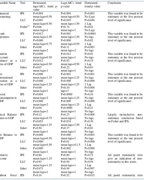
[image:17.612.72.460.209.411.2]

Stationarity Results

Table 1: Stationarity Positions Conclusion Table

Variables Stationarity Position

Financial Deepening I(0)

Trade Openness I(0)

CAB as a ratio of GDP I(0)

NFA as a ratio of GDP I(0)

Social Consumption to GDP I(0)

Fiscal Balance Ratio to GDP Inconclusive, mostly NS

Oil Balance to GDP I(0)

Relative Income I(1)

Labour Force Per Capita Relative Productivity

I(1)

REER I(0)

Imports to GDP Inconclusive, Stationary with lags

Govt. Spending to GDP I(1)

The table above shows a summary of the conclusions from the three unit root tests conducted on

the variables of interest, for more detailed results Table 6 in the Appendices. Three variables,

namely relative income; labour force per capita relative productivity and government spending

were found to be no stationary series while the fiscal balance ratio and the imports to GDP

stationarity tests were largely inconclusive. The variables that were inconclusive or those that

showed signs of a unit root were all differenced and then re-tested after which they were all

stationary at the 1.0 per cent level of significance.

4.4Estimation Techniques: ARDL and Random and Fixed Effects

Both the fixed and random effects estimation techniques will be used in specifying the models

outlined above but the Hausman test will be utilized to choose which of the two techniques offers

20

(18)

17 | P a g e greater efficiency and consistency. In estimating each model, serial correlation and

heteroskedasticity will be controlled for in using the STATA statistical program.

There are two errors which influences a panel framework as noted above, the time constant error

and the random error. The time constant error speaks to the factors that might influence the

model which is indigenous to each sub-panel in the sample and does not vary with time. On the

other hand, the random error has the usual desirous statistical properties of being normally

distributed with mean zero, a constant variance and it is uncorrelated with itself, uncorrelated

with the time constant error and uncorrelated with the explanatory variables.

In applied work, the decision between the fixed effects and random effects is reduced to the

extent to which it is believed that the unobserved time constant omitted variables influences the

panel. Where it is believed that omitted variables may have an impact on the dependent variable,

and may be correlated with the explanatory variables then the fixed effects model is usually used.

The fixed effect technique removes all time constant factors that may influence the variables in

the model and as such there is no need to be concerned about these factors which are usually

unable to be measured. There is also a trade-off between efficiency and consistency when

deciding between the two techniques. The fixed effects model always provides consistent results

but they may not be the most efficient models. The Hausman statistical procedure checks a more

efficient model against a less efficient but more consistent model. The result ensures that the

more efficient model also gives consistent results. Consequently, the Hausman test determines

the optimal trade-off between consistency and efficiency in deciding which test procedure to

utilize.

The ARDL methodology to cointegration was utilized in estimating the Equilibrium REER in the

NATREX approach. This approach is ideal when the aim is to determine the long-run

relationship between two or more variables regardless of their stationarity positions and the size

of the sample. This criterion is critical in this study since the variables being utilized are

integrated of varying order and the sample can be considered relatively small. The ARDL

methodology also accounts for the common problem of weak exogeneity of the regressors

(reverse causality) which ensures that the estimated parameters are efficient and valid contingent

only on the model specification (Pesaran et al., 2001). The ARDL specification can be

(19)

18 | P a g e

∑ ∑

Where Z is a matrix of independent variables.

The first step in evaluating if a long-run relationship exists between the variables included in the

unrestricted error correction model (in equation 10) is to conduct the bounds test proposed by

Pesaran et al (2001). This test involves using a joint F-test in evaluating if the first lag of the

independent and dependent variables have an impact on the dependent variable (Ho: ϕ= =0).

The result from this joint F-test is then compared to the upper and lower bound values purported

by Pesaran, Shin and Smith (2001) at the varying level of significance and also those generated

by Narayan (2005) for smaller samples. The null hypothesis is that the variables are not

cointegrated while the alternative is that a long-run relationship exists between the variables in

the system.

∑

In the case where the system is cointegrated, the long-run and short run models in equations 11

and 12 respectively are estimated and the error correction term which enters the short run model

measures the speed of adjustment back to equilibrium following a shock to the system.

In estimating each of the models identified above, the AIC was utilized to fit the most

appropriate model and autocorrelation, heteroskedasticity and correlation between the time

(20)

[image:20.612.86.429.128.318.2]

19 | P a g e 5.1Empirical Results: Macroeconomic Balance Approach

Table 2: Current Account Norm Equation

VARIABLES Current Account Norm

NFA as a ratio of GDP 3.402*** Exports as a ratio of GDP 31.26** Relative Productivity Index Growth -0.0565* Broad Money to GDP Growth -0.0271 Labour Force Participation 0.312* Fuel Expenditure to GDP -49.05** World Economic Crisis 2008-2009 -2.785** Dummy: High Debt Periods 2.328**

Constant -17.61**

Observations 80

Number of Countries 4

R-squared 0.588

*** p<0.01, ** p<0.05, * p<0.1

In estimating the equilibrium Saving and Investment balance, trade openness, relative income

and fiscal balance were found to be insignificant and as such were omitted from the models. The

impact of the growth of broad money to GDP ratio on the current account was also found to be

insignificant even at the 10.0 per cent level (p=0.22), but had a large practical impact on the

estimated current account norm. The table above shows the variables that were statistically

significant in explaining the medium run current account balance.

The result suggests that a 0.01 increase in the export to GDP ratio increased the current account

norm by 0.3 per cent while a 0.1 increase in the NFA to GDP ratio, improves the current account

balance by 0.3 per cent.21 This suggests that a lower financial debt obligation is conducive to a

more favourable and sustainable current account balance.22 A 1.0 per cent increase relative

productivity index, which implies that the domestic country‟s labour force becomes more

productive relative to its major trading partners, results in a 0.06 per cent reduction in the current

account to GDP ratio. This is an indication that higher income being earned by one countries

labour force relative to another negatively influenced the trade relationship and by extension the

current account.

21

Reducing the debt, the ratio becoming less negative. In the case of the countries in the sample, allowing the ratio to approach zero.

22

(21)

20 | P a g e A 1.0 per cent increase in the labour force participation rate increases the current account balance

by 0.3 per cent while an increase in the fuel expenditure to GDP ratio of 0.01 reduced the current

account by 0.5 per cent. The labour force participation rate is also a proxy of the dependent to

population ratio. Individuals who qualify to be in the labour force but stay outside willingly

(such as discouraged workers) are also considered to be included in the class of individuals who

aid in dissaving in the economy. Therefore, when the labour force increases, this is an indication

of a lower portion of the population being younger or older than the required age criterion for the

labour force or a lower portion of the population being comprised of discouraged workers. The

results therefore highlight that a reduction in these sub-sections of the population improves the

sustainable current account.

The current account was shown to be 2.8 per cent lower during the world economic recession of

2008-2009, which implies that crisis periods pose potential threats to the sustainable level of the

current account. This is because international crisis periods influence the flows of capital, the

level of exports, the price of commodities and the productivity of the labour force. The results

also revealed that when a country had an NFA level that was over -60.0 per cent of GDP, then

their current account surplus were 2.3 per cent higher than the converse.

Forecast Misalignment 2011-2018

The current account misalignment was calculated using the underlying current account forecast

provided by the WEO Database and the current account norm forecast using the parameters

outlined above. For Jamaica and the Dominican Republic, the forecast makes the assumption that

these countries will seek to move to a more sustainable debt position in the medium term and as

such will seek to minimize its NFA to GDP ratio over time. Another major issue which arose in

forecasting the path of the sustainable current account was how to treat countries with increasing

(22)

[image:22.612.72.469.97.274.2]

21 | P a g e Figure 1: Projected Current Account Misalignment (2013-2018) for each panel in the sample

Jamaica and the Dominican Republic were identified as two of such countries and it was

assumed that these countries would address their energy consumption issues by 2016, since the

existing levels were largely unsustainable. The condition is also imposed on these countries that

they will attempt to improve their export to GDP ratio by 1.0 per cent annually in absolute value

over the medium term. Peru‟s norm was projected to be between 6 per cent and 8 per cent higher

than the underlying current account in the medium term and Uruguay‟s projected current account

showed similar misalignment between 4.0 - 6.0 per cent. Jamaica was estimated to have

misalignment between 1per cent and -3.0 per cent over the medium term while the Dominican

Republic had a current account norm which was lower than its underlying medium run current

account between -3.0 per cent and -8.0 per cent.23 The results from the trade elasticities used to

calculate the percentage misalignment of the exchange rate is expressed in the table below. The

trade equation results can be viewed in Table 10 in the Appendices.

Table 3: Trade and Current Account Elasticities

Forecast Elasticities (2013-2018) Import Elasticity

Export Elasticity

Current Account Elasticity

Dominican Republic 0.466 0.8676 0.4283

Jamaica 0.0824 -0.3074 0.5804

Peru 0.5985 0.9805 0.3070

Uruguay 0.1789 0.4504 0.3012

23

See tables 7 and 8 in the appendices for more detailed projections. -10

-5 0 5 10

2013 2014 2015 2016 2017 2018

Projected Current Account Misalignment

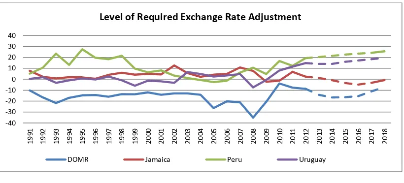
[image:22.612.65.470.574.652.2]

(23)

22 | P a g e Projected Exchange Rate Misalignment

The results indicate periods of strong misalignments, both overvaluation and undervaluation in

all the currencies being evaluated. However, these periods of exchange rates misalignments were

observed to be self-corrective through movements in the macroeconomic fundamentals and

subsequent adjustments in the sustainable current account. This suggests that the misalignment in

the exchange rate is a stationary series and as such is mean reverting. The three unit roots tests

explained in Section 4 above were used to test whether or not this series was explosive. The

results show that this series is stationary at the 5.0 per cent level without a trend, which implies

that misalignment in the current account is self-correcting and does not require excessive policy

action to close. This however occurs due to changes in other macro-economic fundamentals to

equate the underlying and current account norm.

Figure 2 below shows the behavior of the estimated exchange rate adjustment over the sample

period and forecasted to 2018. The forecasted adjustment for Jamaica shows that moving into the

medium term Jamaica will be mildly undervalued; the gap approximately closing in 2018. The

Dominican Republic shows highly significant signs of undervaluation moving into the medium

term, ending at -7.0 per cent in 2018, the major adjustment in 2017 and 2018 highly dependent

and the country correcting its fuel expenditure ratio. Peru and Uruguay both show significant

signs of overvaluation moving into the medium term, with both countries levels of overvaluation

trending upwards and ending at approximately 26.0 per cent and 20.0 per cent respectively in

[image:23.612.73.483.524.710.2]

2018.24

Figure 2: Exchange Rate Misalignment (1990-2018)

24_{The projected path of each countries exchange rate misalignment can be viewed in Table 6 in the Appendices.}

-40 -30 -20 -10 0 10 20 30 40 199 1 199 2 199 3 199 4 199 5 199 6 199 7 199 8 199 9 200 0 200 1 200 2 200 3 200 4 200 5 200 6 200 7 200 8 200 9 201 0 201 1 201 2 201 3 201 4 201 5 201 6 201 7 201 8

Level of Required Exchange Rate Adjustment

(24)

23 | P a g e 5.2Empirical Results: ARDL NATREX Approach

5.2.1 Bounds Test

The estimation of the unrestricted error correction model presented in Section three can be

viewed in Table 8 in the Appendices. In an effort to evaluate whether or not the presented system

is co-integrated, the Pesaran et al (2001) bounds test was utilized. The bounds test suggests

conducting a joint test of significance on the lagged variables in the unrestricted error correction

model. This joint test revealed an F-statistics of F (3, 3) =10.04. This test value was compared to

upper and lower bounds values as outlined in Pesaran, Shin and Smith (2001) in an effort to

determine if the variables included in the system are co-integrated. Pesaran, Shin and Smith

(2001) posit that the asymptotic 1 per cent critical value upper bound for a system with

unrestricted intercept and no trend term is 5.61 where k=3. Narayan (2005) notes that the bounds

presented by Pesaran et al (2001) ought not to be used for small sample sizes and as such he

proposes a smaller upper bound of 5.25 for samples between 30 and 80. Using both upper

bounds, the results confirmed the existence of cointegration at the 1 per cent level of

significance. The next step in the ARDL approach suggests that we estimate the long-run model

as presented in the methodology above.

Long-run Model

The long-run model suggests that the long-run net impact of a 0.1 unit increase in the NFA to

GDP ratio is a 0.02 per cent appreciation of the REER.25 Similarly, a 0.1 unit increase in the

social consumption to GDP ratio of a country appreciates the REER by 0.0011 per cent in the

long-run. Therefore, increase in social consumption has a negligible impact on the REER when

all lagged effects have fully passed through. A one unit increase in the relative productivity index

of a countries labour force appreciates the countries REER index by 0.002 per cent. Surprisingly,

the long-run impact of a 0.1 increase in the fuel expenditure to GDP appreciates the equilibrium

REER by 0.08 per cent in the next period.

25

(25)

[image:25.612.69.414.100.297.2]

24 | P a g e Table 4: Long-run Model

The results above therefore suggest that when a country imports more fuel, increases private or

public spending or becomes less indebted, then their currency will become less competitive

relative to their trading partners. The result also implies that an increase in a countries labour

productivity, relative to its trading partners, may result in a loss in external competitiveness. This

is can be intuitively explained with economic theory. A country‟s NFA improves capital inflows relative to capital outflows, which implies that there is more purchase of foreign assets by

domestic investors relative to foreign investors demand for domestic assets. This improves the

domestic country‟s ability to sustain a stronger REER. The result of the social consumption parameter is suggestive of the Balassa-Samuelson effect whereby increased social expenditure in

the non-tradable sectors relative to the tradable sector resulted in an appreciation of a country‟s currency. However, it is possible that this long-run impact may be different for the varying

countries in the sample and as such future work should focus on country-specific results. The

fuel expenditure impact is also ambiguous and may be panel sensitive. This figure may be due to

the fact that in some countries within the panel, namely Peru, increases in fuel imports are

accompanied by higher levels of fuel exports and higher levels of overall tradable goods exports.

As a result, there are a number of periods of trade surpluses for Peru which may change the

long-run panel impact of this variable. The short long-run impact of all these variables were however

consistent with the literature.

Independent Variables: DV: LN(REER)

NFA 0.572**

Social Consumption 0.185*

RPI 0.00160***

Lagt-1 Fuel Expenditure 0.813**

Lagt-1 NFA -0.414*

Lagt-1 Social Consumption -0.174

Lagt-1 LN(REER) 0.477*

Constant 2.262*

Observations 80

Number of Country Code 4

R-squared 0.429

(26)

25 | P a g e Short Run Dynamics: The Error Correction Term

The error correction term from the short run dynamics model highlighted that the speed of

convergence of exchange rate deviations from its long-run equilibrium following a shock is

approximately 46.2 per cent each year. This is suggestive that the fundamentals which help to

determine the equilibrium exchange rate are automatically manipulated by market conditions to

ensure that exchange rate misalignments are partially corrected within the year. The short run

dynamics regression was estimated with country specific error correction terms and the results

suggested that only Uruguay and Jamaica had a statistically significant speed of adjustment in

the exchange rate when there is a shock to the system. In the country specific equation, the

results suggest that 21.2 per cent and 60.0 per cent of the misalignment in the exchange rate for

Uruguay and Jamaica respectively is corrected per year. For the panel, the half-life deviation

procedure suggests that the length of time it takes the exchange rate to adjust by half following a

shock to the economy was 1.12 years. When the country specific error correction terms were

used, the estimated half-life adjustments were 0.8 years for Jamaica and 2.9 years for Uruguay.

The adjustment suggested by the insignificant half-life parameters of the Dominican Republic

and Peru were 45 years and 145 years respectively. This suggests no adjustment in the exchange

rate following a shock to these economies. This can be explained by the fact that this approach

estimated these currencies as being closely aligned over the sample period.26 The half-life speed

of adjustment found for Jamaica in this study (that is between 0.76 and 1.12 years) coincides

with the finding of Robinson (2010) who found a half-life adjustment between 0.5-1.08 years

using three approaches to calculate the equilibrium RER. Zalduendo (2006) andMacDonald and

Ricci (2003) found a half-life speed of adjust of 2.5 years for Venezuela and South Africa

Respectively. They however note that the speed of adjustment is dependent on the structure of

the economy and the performance of the macroeconomic fundamentals. The result from this

holds critical policy implications since it suggests that if left to itself, exchange rate

misalignments are self-corrective and furthermore, that self-correction is completed over the

short run.

26

(27)

[image:27.612.68.379.96.293.2]

26 | P a g e Table 5: Short Run Dynamics: Full Panel

Independent Variables: DV: Δ LN(REER)

Lagt-1 ECM -0.462**

Δ NFA 0.535**

Δ Social Consumption 0.604** Δ Fuel Expenditure -1.372*

Δ RPI 0.00328*

Lagt-1Δ Fuel Expenditure -0.302

Lagt-1Δ Social Consumption -0.152

Constant 0.0109**

Observations 76

Number of Country Code 4

R-squared 0.467

*** p<0.01, ** p<0.05, * p<0.1

Comparison of Empirical Findings: NATREX and Macro-Balance Approach

The results from the NATREX and the MB approaches are not readily comparable because of

the nature of the underlying assumptions of the two methodologies. The NATREX estimates a

dynamic long-run equilibrium exchange rate that is consistent with macroeconomic

fundamentals while the MB approach estimates the exchange rate misalignment over the medium

term that would ensure internal and external balance simultaneously. Additionally, while the

NATREX is a direct approach to calculating the EREER, the MB approach utilizes an indirect

methodology to calculate exchange rate misalignment. Nevertheless, the two approaches were

consistent in showing that there have been several intervals of misalignment and exchange rate

adjustment over the sample period. Most of the factors which were found to significantly

influence the current account norm, were also found to have long-run relationships with the

REER. The most consistent and important findings between the two approaches is that exchange

rate misalignment is a stationary series which is largely self-corrective. This implies that in the

long-run, there should be no misalignment in the exchange rate since macroeconomic

fundamentals will adjust to ensure that both exchange rate and current account gaps are closed.

Finally, the resulting equilibrium exchange rates were highly similar using the two approaches,

with deviations occurring mainly between recessionary periods.27

27

(28)

27 | P a g e 6. Conclusion and Policy Implications

The study found that the critical factors influencing the sustainable levels of the current account

included a country‟s NFA to GDP ratio, relative productivity growth, labour force participation and fuel to GDP ratio. World economic crisis periods were also found to significantly reduce the

sustainable levels of the current account, which can be explained by shocks to the flow of capital

during these periods. The results from this study also revealed that there have been a number of

years over the sample period where the current account for the various countries has been

significantly misaligned. As a result, the MB approach has found that the exchange rates for each

of the countries in the study have had significant periods of misalignment from the ERER. The

required level of exchange rate adjustment was found to be a stationary series over the sample

period, which confirmed the assumption that in the long-run, a current account misalignment and

by extension an exchange rate misalignment from its equilibrium positions, should be

self-corrective.

The NATREX approach similar to the MB approach found that the EREER was determined by a

country‟s net assets, the level of government and foreign consumption, the effectiveness of the labour force and the fuel expenditure of the country. Shocks to the EREER were found to be

self-corrective for all countries in the sample (negative error correction term) but significant

corrections were only found for Jamaica and Uruguay. The speed of adjustment was found to be

relatively quick based on both the half-life deviation and the error correction term.

These findings hold a plethora of implications for policy discussions moving forward. The most

notable among these is the self-corrective nature of exchange rate misalignment found by both

procedures. The implication of this is that since the real exchange rate is determined by long-run

macroeconomic fundamentals, exchange rate misalignment will be corrected through the

behaviour of these variables. The second notable implication is that less emphasis should be

placed on exchange rate misalignment as the sole factor influencing current account

misalignment. The results implicitly show that a current account misalignment may also rest on

the macroeconomic fundamentals which determined the sustainable levels of the current account.

Consequently, the question which policy makers should carefully examine is the extent to which

these fundamentals are performing optimally and whether price adjustment is the only factor

(29)

28 | P a g e findings of this study suggests that price competitiveness is by no means the only factor which

produces a favorable current account. This is seen by the fact that the countries in the sample

have had several periods of both undervaluation and overvaluation. However, the current account

has not responded to these periods of misalignment. In the case of Jamaica for example, the

current account has steadily deteriorated despite fluctuations in the REER and periods of

misalignments in both direction. Therefore, the structural factors influencing the current account

must be evaluated rather than looking to price competitiveness as the only means of restoring

(30)

29 | P a g e References

Pineda, E., Cashin, P., Sun, Y., & International Monetary Fund. (2009). Assessing exchange rate competitiveness in the eastern Caribbean currency union. Washington, D.C.: International Monetary Fund.

Coudert, V. & Couharde, C.. (2005). Real equilibrium exchange rate in China. Paris: CEPII.

Driver, R. L., Westaway, P., & Bank of England. (2004). Concepts of equilibrium exchange rates. London: Bank of England.

Dunaway, S. V., Li, X., & International Monetary Fund. (2005). Estimating China's "equilibrium" real exchange rate. Washington, D.C.: International Monetary Fund, Asia and Pacific Dept. and Policy Development and Review Dept.

Eckstein, Z & Friedman, A. (2011). The equilibrium real exchange rate for Israel. Bank of Israel: Papers No 57.

Edwards, S. (1989). Real exchange rates devaluation and adjustment. London: MIT Press.

gert, . Halpern, L. (2005). Equilibrium exchange rates in Central and Eastern Europe. London: Centre for Economic Policy Research.

gert, ., Halpern, L., MacDonald, R., Oesterreichische Nationalbank. (2005). Equilibrium exchange rates in transition economies: Taking stock of the issues. Vienna: Oesterreichische Nationalbank.

Fida, B et al. 2012. 'Estimating Equilibrium Real Exchange Rate through NATREX Approach: A case of Pakistan. Journal of Basic and Applied Scientific Research 2(4) p. 3642-3645.

Graham, J and Steekamp, D. (2012). Extending the Reserve ank‟s macroeconomic balance

model of the exchange rate. Retrieved from

http://www.rbnz.govt.nz/research_and_publications/analytical_notes/2012/an2012_08.pd f on July 20, 2013.

Henry and Longmore. (2003). Current Account Dynamics and the Real Effective Exchange Rate. Research and Economic Planning Division: Bank of Jamaica.

Hojman, D. (July 01, 1989). Fundamental Equilibrium Exchange Rates under Contractionary Devaluation: A Peruvian Model. Journal of Economic Studies, 16, 3.)

Husted, S. L., & Melvin, M. (1990). International economics. New York: Harper & Row.

IMF. (April 2013). World Economic Outlook Database. Retrieved from

(31)

30 | P a g e IMF. (2008). De Facto Classification of Exchange Rate Regimes and Monetary Policy

Frameworks. Retrieved from

https://www.imf.org/external/np/mfd/er/2008/eng/0408.htm on June 13, 2013.

Isard, P et al. (2001). Methodology for current account and exchange rate assessments. Washington, DC: International Monetary Fund.

Karadi, Peter. (2003). Structural and Single Equation Estimation of the NATREX Equilibrium Real Exchange Rate, Central Bank of Hungary, Working Paper.

Lee, J et al. (2006). Methodologies for CGER exchange rates assessment. Washington, DC: International Monetary Fund.

Levin, A., C.-F. Lin, and C.-S. J. Chu. 2002. Unit root tests in panel data: Asymptotic and finite-sample properties. Journal of Econometrics 108: 1–24.

MacDonald, R., and L. Ricci. (2003). Estimation of the Equilibrium Real Exchange Rate for South Africa. IMF Working Paper 03/44 (Washington: International Monetary Fund).

Maddala, G. S., & Wu, S. (January 01, 1999). A Comparative Study of Unit Root Tests with Panel Data and a New Simple Test. Oxford Bulletin of Economics and Statistics, 61, 631.

Montiel, P., & United Nations. (2007). Equilibrium real exchange rates, misalignment and competitiveness in the Southern Cone. Santiago Chile: Naciones Unidas, CEPAL, Economic Development Division.

Narayan, P.K., (2005), “The saving and investment nexus for China: Evidence from cointegration tests”. Applied Economics, 37: 1979–1990.

Nowak-Lehmann D., Felicitas, Herzer, Dierk, Vollmer, Sebastian, Mart nez-Zarzoso, Inmaculada. (2011). Modelling the Dynamics of Market Shares in a Pooled Data Setting.

Pesaran, M. H., Shin, Y., & Smith, R. J. (2001). Bounds Testing Approaches to the Analysis of level Relationships. Dae Working Papers, 7.

Robinson, J. (2010). Determining the Equilibrium Exchange Rate for Jamaica: A fundamentalist approach. Research and Economic Planning Division: Bank of Jamaica.

Siregar, R. Y., & South-East Asian Central Banks. (2011). The concepts of equilibrium exchange rate: A survey of literature. Kuala Lumpur: South East Asian Central Banks (SEACEN) Research and Training Centre.

(32)

31 | P a g e STATA. (2011). LONGITUDINALDATA/PANEL DATA REFERENCE MANUAL. STATA Press: Texas.

Stein, J. L. (2005). The transition economies: A NATREX evaluation of research. M nchen:

CESifo.

Stein, J. L. (2001). The equilibrium value of the Euro, $ US exchange rate: An evaluation of research. Munich: Univ., Center for Economic Studies.

Stein, J.L. (1994). “The Natural Real Exchange Rate of the US Dollar and Determinants of

Capital Flows” in J. Williamson (ed.), Estimating Equilibrium Exchange Rates,

Washington, D.C.: Institute for International Economics.

United Nations Statistics Division. (2013). UNDATA. Retrieved from

http://data.un.org/Default.aspx on June 13, 2013.

Williams, P. (June 2008). Estimating Jamaica’s Real Equilibrium Exchange Rate. Bank of

Jamaica Working paper retrieved from

http://www.boj.org.jm/publications/research_papers.php on June 11, 2013.

Williamson, J. (1994), “Estimates of FEERs,” in J. Williamson (ed.), Estimating Equilibrium Exchange Rates, Washington, D.C.: Institute for International Economics.

(33)

[image:33.612.114.500.144.366.2]

32 | P a g e Appendices

Figure 3: Trends in Selective Economic Data: Jamaica

Figure 4: Trends in Selective Economic Data: Peru

-30 -20 -10 0 10 20 30

0 20 40 60 80 100 120 140 160

Jamaica's REER, Exports and CAB Trends

REER INX (LHS) CAB_%GDP (RHS)

Oil Expen. % GDP (RHS) Export % GDP (RHS)

-15 -10 -5 0 5 10 15 20 25 30

0 20 40 60 80 100 120 140