A Simple Jerky Dynamics, Genesio System
Ömür Umut, Serpil Yaşar
Department of Mathematics, Faculty of Arts & Sciences, Abant Izzet Baysal University, Bolu, Turkey Email: [email protected], [email protected]
Received October 31, 2012; revised December 10, 2012; accepted December 19,2012
ABSTRACT
The third order explicit autonomous differential equations named as jerk equations represent an interesting subclass of dynamical systems that can exhibit many major features of the regular and chaotic motion. In this paper, we show that an algebraically simple system, the Genesio system can be recast into a jerky dynamics and its jerk equation can be de- rived from one-dimensional Newtonian equation. We also investigate the global dynamical properties of the corre- sponding jerk system.
Keywords: Genesio System; Algebraically Simple Systems; Jerky Dynamics; Newtonian Jerky Dynamics; Dynamical Properties
1. Introduction
The term jerk [1], i.e., the third derivative of displace- ment, x, has attracted some attention because of its relevance to the theory of chaos [2-11]. Some papers appeared in response to a question [2] posed by Gottlieb concerning simple jerk functions which may lead to cha- otic phenomena. Sprott [3,4] found several simple non- linear jerk functions which gave strange attractor for ap- propriate choices of equation parameters and initial con- ditions. Linz [5,6] introduced the idea and conditions for Newtonian jerky dynamics, derivable by differentiation of a (one-space dimension) Newtonian equation of mo- tion for x, and analyzed the jerky dynamics for one- variable obtained from several familiar autonomous sys- tems of three simultaneous first-order ordinary differen- tial equations which are known to have chaotic solutions. He also allowed for the possibility of a memory or tem- poral history integral term in the force function. Coinci- dentally, Maccari [7] had considered such generalized oscillators, with nonlocal force terms, which obeyed an integro-differential equation and which were equivalent to an autonomous third-order nonlinear differential equa- tion. His interests there were in periodic and quasi-peri- odic solutions.
As jerky dynamics can be considered a subclass of three-dimensional dynamical systems an interesting ques- tion [5] is which three-dimensional systems are equiva- lent to jerky dynamics. In [8], a class of three-dimen- sional nonlinear dynamical systems is studied which can be transformed into jerky dynamics. Most of the models of minimal chaotic dynamics considered in [8] belong to this class and can be transformed into jerky dynamics.
The transformations used have the restriction that the variable in the scalar differential equation is the same as the system. A consequence is that a linear transformation is sometimes not possible; the resulting transformation is nonlinear. In [9], it is shown that by removing this re- striction, these models can be transformed to jerky dy- namics via an affine transformation.
In [8], Eichhorn et al. used the method of Gröbner bases and showed that fifteen of Sprott’s chaotic flows [4] can be recast into a jerk form. They also showed that these fifteen models, Sprott’s minimal chaotic flow [4] and the Rössler toroidal model [10] can be arranged into seven classes (referred as JD1 to JD7) of jerky dynamics
as a hierarchy of quadratic jerk equations with increas- ingly many terms as seen in Table 1. Such a classifica- tion provides simple means to compare the functional complexity of different systems and also demonstrate the equivalence of cases not otherwise apparent. In a subse- quent study, Eichhorn et al. [11] examined the simplest cases of JD1 and JD2 in more detail and identified the
regions of parameter space over which they exhibit chaos. In this paper, we show that the Genesio system can be recast into a jerky dynamics by an affine transformation and the resulting form belongs to class JD2. Moreover it
is derived from one-dimensional Newtonian equation that is, it is a Newtonian jerky dynamics. Furthermore we investigate the global dynamics of that jerk equation and also show that it shares the common route to chaos as systems in class JD2.
2. Jerky Dynamics
CTable 1. Basic classes of dissipative jerky dynamics.
Model Basic classes coefficients = values for which there is irregular behavior Transformation
JD1 k1k2 k3
I k1 1 k2 2 0.4 8
2
3 2 0.0
k 2y
J k1 2 k2 4 k31 4 2y 1
L k1 1 k2 3.9 k3 2 8.19 2x
N k1 2 k2 4 k3 2 4 2z
R k1 1 k2 0.9 k3 0.4 x
SJ k1 A 2.017 k2 1 k30 v
JD2 k1k2 2k3
M k1 1 k2 1.7
2
3 4 2.4225
k
2 x
Q k1 1 0.5 k2 2.6
2
3 4 2.4025
k
2 y
S k1 1 k2 4
2
3 16
k z
TR k1 0.2 k2 1
2 3
1 4 0.0858 k
1 2 y
GS k1 c k2 b
2
3 4
a k
2 a x
JD3 k1k2k32k4
F k1 1 0.5 2
1 1 2.5
k
k3 2 0.25
4
1 1
2 k
2x 1
G k1 1 0.6 2
1
1 1.85 2
k
k3 0.4 4
1 0.625 4 k
1
2 x
H k1 1 0.5 2
1 1 2.5
k
k3 2 0.25
4
1 1
2 k
2z 1
JD4 k1k2k32k4
O 1
1 2
k k2 1 1.7 k3 1 4
1 4
k 1
2 x
JD5 k1k22k32
D k1 1 k2 1 k3 3 x
JD6 k1k2k32k42k5
.7
P k1 1 k2 1 1 3
1 2
k k41 5
1 2
k 2y1
JD7 k1k2k32k42k5 k6
K 1
1 1
2 2.37
k
2
1 1
2 3.53
k
3 0.3
k k41 k5 2 1.7 6
1 0.83 4 k
1
2 y
scalar ordinary differential equations:
n f
, , , , 1
n
(1)where n is the order and n denotes the nth derivative
of the scalar state variable . Clearly an nth order scalar ODE can be written as a system of n first order ODEs. On the other hand, the following systems of equations can be rewritten as a scalar ODE:
0 1 1
0 0 1
. 0 0 1
n f x
p p p
x x
For third order
n3 scalar ODEs, where is position, is the change in acceleration which is gen- erally called the jerk, and the resulting dynamics are called jerky dynamics. In [8], a class of three-dimen- sional dynamical systems is considered whose members are topologically conjugate to jerky dynamics.Theorem 2.1 Consider a three-dimensional system of the form
A
x x n x (2) where x3, A3 3
, 1, 2,3
is a matrix with constant coeffi-
cients ij and
a three-dimensional vector solely nonlinear functions in x, y, z that are twice differentiable and do not contain addi- tive constants. If
a i j n x
n1
x ,n2 x ,n3 x
T
12 2 13 3 , 12 13
a n x a n x f x a y a z (3) and
2 2
12 23 13 32 12 13 33 22 0
a a a a a a a a (4)
then the system is topologically conjugate to a jerky dy- namics via a state transformation.
The state transformation in Theorem 2.1 has the re- striction that the state variable in the corresponding jerky dynamics f
, ,
is equal to one of the state variables in Equation (2). It was shown that 16 out of 20 simple chaotic systems considered in [8] fall into this class and thus are equivalent to jerky dynamics. For some of these systems, the corresponding state transfor- mations are necessarily nonlinear. This is due to the above restriction on the state transformation. In [9] it was shown that without this restriction, simple linear trans- formations can be found which transform these systems into jerky dynamics. In particular, the following result gives sufficient conditions under which an n-dimensional system is topologically conjugate to a scalar ODE via an affine state transformation.Definition 2.1. Let A be an n by n matrix and b be an n by 1 vector. The pair
A,b is controllable if the matrix
,
| | 2 | | n1
K Ab b Ab A b A b
is nonsingular. The matrix K is called the controllability matrix.
Theorem 2.2. Consider the system
A f
x x b x c
(5)
where A is an n by n matrix, b, c are n by 1 vectors and f is a real-valued function. If is controllable, then the system is topologically conjugate to a scalar ODE via an affine transformation.
A,bIt is possible that a dynamical system that is contained in the class specified by Equation (5) can be converted simultaneously into two or three jerky dynamics in dif- ferent variables (the jerky dynamics in the certain vari- able is unique, if it exists).
To obtain dynamical systems of the class in Theorem 2.2 with two simultaneously existing jerky dynamics, e.g., in x and y one has to restrict the nonlinear function
2n x such that it is only function of y, i.e., n2
x
2
n y . This follows directly from Equation (2). In addi- tion to the conditions (3) and (4)
12 2 13 3 1 , 12 13
a n y a n x f x a y a z
(6)
2 2
12 23 13 32 12 13 33 22 0
a a a a a a a a (7) that ensure the existence of the jerky dynamics in x, there are also corresponding constraints for the jerky dynamics in y that read explicitly
21 1 23 3 2 , 21 23
a n x a n x f y a x a z (8)
2 2
23 31 21 13 21 23 11 33 0
a a a a a a a a (9) where f1 and f2 are functions of the indicated arguments.
Any dynamical system of functional form (5) with
2 2
n x n y that fulfills the conditions (6)-(9) can be recast into an equivalent jerky dynamics in its variables x and y. For simultaneously existing jerky dynamics in two other variables one has to take into account permutations of variables and indices, respectively.
For dynamical systems that possess simultaneously three jerky dynamics, further constraints apply. Clearly,
3 3
n x n z must hold. Furthermore, in addition to Equations (6)-(9) there is a third condition reading ex- plicitly
31 1 32 2 3 , 31 32
a n x a n y f z a x a y
(10)
2 2
31 12 32 21 31 32 22 11 0
a a a a a a a a (11) If a jerky dynamics can be derived from one-dimen- sional Newtonian equation by taking its derivative with respect to time we call the dynamics Newtonian jerky. The following theorem [6], states under which conditions a jerky dynamics can be Newtonian jerky:
form
,
,xp x x x q x x
0 (12) with p and q being differentiable and integrable func- tions of their arguments x and x, is Newtonian jerky.
In the qualitative theory of dynamical systems [12,13] gradient systems play an interesting role. For these sys-tems, one can rule out the existence of oscillatory solu-tions just by considering their vector fields. In particular, a dynamical system is a gradient system if its vector field results from the gradient of a scalar potential. In [6], it is shown that there is no elementary criterion that excludes periodic solutions in some classes of Newtonian jerky dynamics.
Theorem 2.4. Newtonian jerky dynamics are not gra- dient systems.
Looking at the functional form of a jerky dynamics, it is highly nontrivial to decide whether it can have chaotic solutions for some parameter ranges or not. For some subclasses of jerky dynamics one can derive a simple criterion under what circumstances aperiodic or chaotic solutions cannot appear. Consider the jerky dynamics (12) with
, ,
q x x r x x x s x x ,
(13)
where r and s are functions of the indicated arguments and r x x
, fulfills the Schwarz condition xp x x
, x . As a consequence the jerky dynamics (12) can
be rewritten as
,r x x
,
,
,xp x x x r x x x s x x
(14) or equivalently,
d , d d , d .
d d
x t
x p x x x s x x
t
t
(15)
Direct integration of Equation (15) yields
, d
, d .x t
x
p x x x
s x x (16) This shows most clearly that the left-hand side of Equation (16) can be interpreted as an oscillator coupled to an internal driving mechanism or feedback (the right- hand side of Equation (16)) that is an integral over the history of its motion. This fact has some consequences for the possible dynamics of the jerky system (15).
Theorem 2.5. [6] If 1) the oscillator on the left-hand side of Equation (16), , possesses only bounded solutions and 2) the integrand of memory term,
, d 0x
x
p x x x
,s x x , on the right-hand side of Equation (16) is either positive semi-definite or negative semi-definite for all x and x, then the jerky dynamics (15) cannot show chaotic behavior.
3. Genesio System as Jerky Dynamics
The Genesio system, which was proposed by Genesio
and Tesi [14], is described by the following simple three- dimensional autonomous system with only one quadratic nonlinear term:
2
, ,
xy yz z ax by cz x (17) where a, b, c are real parameters.
Theorem 3.1. The Genesio system (17) can be recast into a jerky dynamics, and the resulting form belongs to class JD2.
Proof. The Equation (17) can be written as
A f
x x b x c
,
c
(18) where
0 1 0 , 0 0 1
x y A
z a b
x
20 0
0 , 0 , . 1 0
f x x
b c
The matrix
2
0 0 1 , 0 1
1
K A
c c b
b c is nonsin-
gular since det
K 1 0. So, by Definition 2.1 K is the controllability matrix and the pair
A,b
is control- lable. Hence the Genesio system can be recast into a jerky dynamics via an affine transformation by Theorem 2.2.Application of the invertible transformation x y y z
to the Equation (17) yields
2.
x cx bx ax x
(19) Using the linear and invertible transformation
, , 2
a
x x
x (20)
and then replacing by x we write Equation (19) as
2 2
4 a
x cx bx x
(21)
Comparing with Table 1, one can see that the resulting jerk equation belongs to the class JD2 with
2 1 , and2 3 .
4 a k c k b k
Theorem 3.2. Genesio system has no equivalent jerky dynamics in the variables y and z.
Proof. For a simultaneous existence of jerky dynamics in y and/or z first, the following conditions must be satis- fied:
2 2 and or 3 3
For the Equation (16) we have
2 0 and or 3
n x n x 2
3 .
x n z
Since the second equation in (22) does not ho we can concl
ld
ude that the Equation (17) cannot have a jerky dy- namics in z.
From the condition (8) we get
2 2 ,f y z x which is absurd. This follows that the Gene have a jerky dynamics in y also.
Theorem 3.3. The Genesio system is a Newtonian jerky dynamics.
sio system cannot
where
Proof. The Equation (21) can be put in the form (12)
,
, 0xp x x x q x x
,p x x c and
2 2 x , 4 a
q x x bx . Since nd q are dif e and integrable fun
both p a ferentiabl ctions of their arguments x and x the jerky dynamics (21) is Newtonian by Theorem 2.3.
Corollary 3.1. The Genesio system is not a gradient system.
Proof. From Theorem 3.3 we know that the Genesio system is a Newtonian jerky. Since Newtonian jerky dy- namics are not gradient systems by Theorem 2.4, the Genesio system is not a gradient system.
Theorem 3.4. The Genesio system exhibits chaotic so- lutions for some parameter ranges.
Proof. We can write Equation (21) as
2 2 a
x cx bx x
4 (23) Integration of Equation (23) yields
2 2d
t a
x cx x
4
The memory term
2 2 4 ax changes sign as x varies,
th ositive
semi-definite for all x. Therefore the Genesio system can
al Properties
at is, it is neither p semi-definite nor negative
have chaotic solutions for some parameter ranges by Theorem 2.5.
4. Dynamic
Given the jerky dynamics
2
2 0
4 a x cx bx
x (24)
the equilibria can be found by assum
fixed point , , , which leads to ing that it has a x x0 x0
22
, 0, 0 a 0
J x x
4 , or 2
a
x . So there are two
equilibria: ,0,0 2
a E
and ,0,0
. Linearizing
Equation (2 e equilib provides one real and a p plex co values along
2
a E
4) about th rium air of com njuga n
n E te eige with the following characteristic equatio
3 c 2 b a 0
(25) and linearizing the Equation (24) about the other equilib- rium E yields the following characteristic equation
3 c 2 b a 0.
(26) According to Routh-Hurwitz criteria, the equilibrium
is stable (i.e., the real part of all
E roots i
i1, 2,3
of Equation (25) are negative) only if the conditions
0, 0, 0, 0
a b c bc a ) are fulfilled. For bc a a 0, ,
b c 0
(27
, the fixed point becomes unstable and the two compl
axes, while the third r
ex roots of (25) cross the imaginary oot remains real and negative. Therefore at bc a a stable limit cycle arises via a Hopf bifurcation.
E has the same stability characterization. If
0, 0, 0,
a b c bc a 0 (28)
then criteria
and at
Equation (26) satisfies the Routh-Hurwitz bc a a stable limit cycle arises
lume
via a Hopf bi- furcation.
The vo contraction rate of the Equation (24) is
2
2 ,
4
x cx bx x c
a 1 d d V c
V t ,
i.e., which can be solved to yiel d
0 ectV t V tion (24) is that contract at a
. When is positive, the jerky d Equa dissipative with solutions for
c ynamics
t
a limit n exponential rate c onto an attractor of zero volume that may be an equilibrium point, cycle, or a strange attractor. When c 0, is zero and the phase space volume conserved and the dynamical system is conservative. When c is negativ
=
e, is posi- tive and the volume expands exponentially fast and there are only unstable fixed points. Therefore the ynamics diverges for t if the initial value does not lie ex- actly at such unstable set.
The Equati n ( ) has three free parameters a, b and c
and the position of equilib
d
o 24
ria ,0,0 , ,0,0
2 2
a a
E E
o get the parameter inde ransformation
depends on the parameter a. T - pendent equilibria we use the t
2 ,
x x t ct a
(29)
for x and t yielding the new quantities x and t. With the ation (24) becomes substitution of Equation (29), Equ
2 2 3 1
b a
x x x x
c c
2
2, b c
3
2
a c
introducing as new pa meters and
dropping the overbars we write
tionary points ra
x21 .
(30)Equation (30) possesses two sta x x x
1
x ,
0
x
, characte
0
x
. Analyzing their stabi
is stable only for
lity leads to the ristic equation
3 2 2 0.
(31) It follows that x1 0 ,
0
and 2
viaand it becomes unstable at the line
2 0, 0 a Hopf bifurcation. Sim
1
is stable only for 0
x , 0 and ilarly, 2
becom he line 2
0, 0
and it es unstable at t
. These stability properties of fixed o reflect the symmetry of the Genesio system.
s invariant under via a Hopf bifurcation
points als
Equation (30) i x x and . Therefore, knowing the solution of x t
of Equation (30) for a certain value of parameter and certain ini- tial values, the dynamics of the correspondingverted
sign in-
and initial values is given by x t
.Summarizing the results, we conclud that possibly interesting dynamics of the Genesio system (17) is de- scribed by Equation (30). Due to the discussed symmetry of this equation, we need only to consid
e
er initial values close to one of the two stationary points. Then the most interesting region of the
,
-parameter plane is the one for 2 and positive . From the studies in [11,15,16], we also know that this parameter region con- tains homoclinic orbits of the other stationary point1
x , x0
, x0
, which here is also a saddle- focus.
5. Numerical Results
Besides the local stability and Hopf bifurcation analysis of Equation (30), we also computed the set of all Ly-
ent values of parameters apunov exponents for differ
and and use to determine and classify the long-time dynamics of the Genesio system. Numerical calculations are performed using Mathematica and iDMC softwares, and RKF45 and RK2Imp are used as numerical algo- rithms with step size 0.001. The initial values are chosen as x1.005, x0.05
, x0.05
which are close to the fixed point x1, x0
, x0
.
For the parameter regions 0 or 0, no bounded solutions have been found. This suggests that the Gene- sio system does probab posse s at all a stable at- tractor in thes io r gi
ly not s
e reg ns. Fo the re on 0 and
0
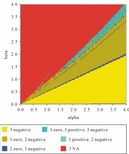
[image:6.595.311.534.82.347.2] the resulting Lyapunov spectra are shown in Figure 1. The fixed point domain is followed by a large limit cycle region and a structured chaotic region. How- ever the chaotic region is not present for 1.6. At
Figure 1. Lyapunov spectra for the jerky dynamics Equa- tion (30).
its boundary is formed by two tongues tha
e only finds chaotic points at
1.6
t
reach into the limit cycle domain. For smaller parameter
values on 0.75 and
0.71
. Moreover there are islands with y- namics
urcation gram wh
bounded d (limit cycles and strange attractors) located with- in the diverging region.
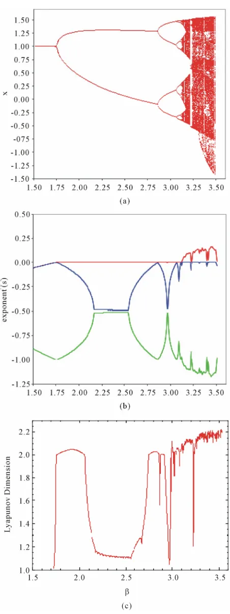
In Figure 2(a), we have shown the bif dia- ich is the plot of successive maxima of the long time evolution of x t
as a function of system parame- ter for fixed value of the parameter 3.5pf bifur
. By Fig- ure 2(a), it becomes clear that the jerk dynamical system Equation (30) having quadratic nonlinearity shows the chaos with a cas of period-doubling bifurcations which is initiated by a supercritical Ho cation at the line 2
cade
. Therefore the limit cycle domain that follows the fixed point region
1.5 1.75
, consists of periodic attractors with period 2n
nN
, 1.75 < < 3.142.
This re onsists of an infinite series of period- doubling bifurcations. It also y narrow windows, which are called limit cycle windows. As
gion c
contains man
is further increased the limit cycle windows break an
down d eventually disappear. In Figure 2(b), the Lyapunov exponents as a function of the parameter is for the same range as that of the bifurcation plot. In Figure 2(c the Lyapunov dimension is for the same range of
),
as
where the bifurcation diagram shows the limit cycle so- lutions, the largest Lyapunov exponent is negative as well as the dimension of the attractor is two. However, for the values of the parameter where the bifurcation plot shows the existence of aperiodic behavior (chaotic), the largest Lyapunov exponent is positive as well as the dimension of the attractor is a non-integer 2.15119 be- tween two and three for the parameter values 3.5
and 3.46.
For a computed value of , we record the successive local maxima of x t
for a trajectory on the strange attractor. Figure 3 shows xn1 vs xn, where xno de
e nth r all
l tain
r - notes th local maximum. The data points f nearly on a one-dimensiona curve. These one-dimen- sional maps are ob ed to compare the different dy- namics on a dynamical system. Such maps with pa abola like maxima are well-known for the generation of the chaotic solution through period-doubling route and it gives us a clue the route to chaos in the jerk dynamical systems under consideration.
Figure 4 shows two-dimensional projections of the system’s attractor for different values of (with
3.5
held fixed). At 2.5 the attractor is a stable limit cycle. As is decreased to 3.0, the limit cycle goes around twice before closing, and its period is ap- proximately twice that of the original cycle. This is what peri oubling looks like ontinuous-time system. In fact, somewhere between 2.5
od-d in a c
and 3.0, a period- doubling bifurcation of cycles must have occurred. An- other period-doubling bifurcation creates the four-loop cycle shown at 3.1. After an infinite cascade of fur- ther period-doublings, we obtain strange attractor at
3.46
the
[image:7.595.59.285.78.681.2] .
Figure 2. Behavior of the jerk dynamical system having quadratic nonlinearity Equation (30) for a fixed value of the parameter α = 3.5. (a) The bifurcation diagram; (b) The Lyapunov exponents; (c) The Lyapunov dimension of th
[image:7.595.308.540.493.730.2]β = 2.5 β = 3.0 β = 3.1
[image:8.595.59.289.85.219.2]β = 3.12 β= 3.23 β = 3.46
Figure 4. Two-dimensional projections of the attractor of the Equation (30) for different values of β.
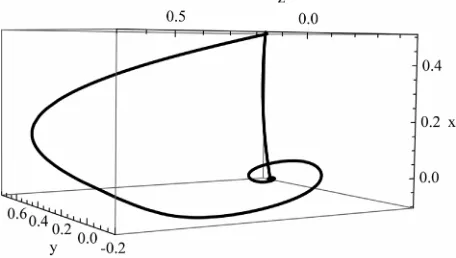
Figure 5. Homoclinic orbit of the Equation (30).
The underlying variety of dynamical behavior can be related to the occurrence of homoclinic orbits as sh in Eichhorn et al. [11] and Glendinning and Sparrow
[15] le
em is likely rmined by the interactions between the stable and un-stable manifolds of the single stationary point leading, finally, to homoclinicity.
6. Discussion
In this paper, we showed that Genesio system is one the functionally simplest polynomial classes of jerky dynamics, JD2 and it is a Newtonian jerky dynamics.
also investigated some aspects of the dynamical pr ties of the Genesio system and we have found for this system there are not only few parameters but wide ra g of parameter values that lead to chaotic long time dy-
namic
pre-nt where the long time attractor of the dynamics si
is associated with the appear- ance of various homoclinic orbits as in the works of
1], Glendinning and Sparrow [15] and
own , . In fact, with a numerical search we have been ab to detect homoclinic orbits as depicted in Figure 5. Hence the dynamics of the Genesio syst de- te
of
We oper-
n es
s. Moreover, also large parameter regions are
se con-
sts of stable limit cycles. The route to chaos is deter- mined by a period doubling cascade (for appropriately varied system parameters) that is initiated by a Hopf bi- furcation. Varying the initial conditions, we are also able to detect several coexisting stable attractors. Therefore, despite its functional simplicity, the Genesio system
shows a rich diversity of dynamical behavior.
We have seen that the complexity and diversity of the dynamics of Equation (30)
Eichhorn et al. [1 Arneodo et al. [16].
REFERENCES
[1] S. H. Schot, “Jerk: The Time Derivative of Change of Acceleration,” American Journal of Physics, Vol. 46, No. 11, 1978, pp. 1090-1094. doi:10.1119/1.11504
[2] H. P. W. Gottlieb, “Question #38. What Is the Simplest Jerk Function That Gives Chaos?” American Journal of Physics, Vol. 64, No. 5, 1996, p. 525.
doi:10.1119/1.18276
[3] J. C. Sprott, “Some Simple Chaotic Jerk Functions,”
American Journal of Physics, Vol. 65, No. 6, 1997, pp. 537-543. doi:10.1119/1.18585
[4] J. C. Sprott, “Simplest Dissipative Chaotic Flow,” Phys- ics Letters A, Vol. 228, No. 4-5, 1997, pp. 271-274.
doi:10.1016/S0375-9601(97)00088-1
[5] S. J. Linz, “Nonlinear Dynamics and Jerky Motion,”
American Journal of Physics, Vol. 65, No. 6, 1997, pp. 523-526. doi:10.1119/1.18594
[6] S. J. Linz, “Newtonian Jerky Dynamics: Some General Properties,” American Journal of Physics, Vol. 66, No. 12, 1998, pp. 1109-1114. doi:10.1119/1.19052
[7] A. Maccari, “T ,” Nuovo Cimento
B, Vol. 111, N
he Non-Local Oscillator o. 8, 1996, pp. 917-930.
doi:10.1007/BF02743288
[8] R. Eichhorn, S. J. Linz and P. Hanggi, “Transformations of Nonlinear Dynamical Systems to Jerky Motion and Its Application to Minimal Chaotic Flows,” Physical Review E, Vol. 58, No. 6, 1998, pp. 7151-7164.
doi:10.1103/PhysRevE.58.7151
[9] C. W. Wu, “On Nonlinear Dynamical Systems Topologi- cally Conjugate to Jerky Motion via a Linear Transforma- tion,” Physics Letters A, Vol. 296, No. 2-3, 2002, pp. 105-108. doi:10.1016/S0375-9601(02)00267-0
[10] O. E. Rössler, “Continuous Chaos: Four Prototype Equa- tions,” Annals of the New York Academy of Sciences, Vol. 316, No. 1, 1979, pp. 376-392.
doi:10.1111/j.1749-6632.1979.tb29482.x
2002, pp. 1-15.
[11] R. Eichhorn, S. J. Linz and P. Hanggi, “Simple Polyno- mial Classes of Chaotic Jerky Dynamics,” Chaos, Soli- tons & Fractals, Vol. 13, No. 1,
doi:10.1016/S0960-0779(00)00237-X
[12] L. Perko, “Differential Equations and Dynamical Sys- tems,” Springer-Verlag, New York, 1991.
doi:10.1007/978-1-4684-0392-3
[13] J. Hubbard and B. West, “Differential Equation
namical Systems Approach,” Springer-Verlag, New York, s: A Dy- 1995. doi:10.1007/978-1-4612-4192-8
[14] R. Genesio and A. Tesi, “Harmonic Balance Methods for the Analysis of Chaotic Dynamics in Nonlinear Systems,”
[image:8.595.58.286.262.391.2]-H doi:10.1016/0005-1098(92)90177
[15] P. Glendinning and C. Sparrow, “Local and Global Be- havior near Homoclinic Orbits,” Journal of Statistical Physics, Vol. 35, No. 5-6, 1984, pp. 645-696.
doi:10.1007/BF01010828