Munich Personal RePEc Archive
The Impact of Minimum Wage on
Average Earnings in the Caribbean using
Two-Selected Countries, Trinidad and
Tobago and Jamaica (1980-2011 and
1997-2011)
Bamikole, Oluwafemi
The University of the West Indies, Caribbean Policy Research
Institute
10 January 2013
Online at
https://mpra.ub.uni-muenchen.de/57363/
1
The Impact of Minimum Wage on Average Earnings in the Caribbean using Two-Selected Countries, Trinidad and Tobago and Jamaica (1980-2011 and 1997-2011)
Oluwafemi O. Bamikole1
January, 2013
…it is no kindness to the workers in a trade to merely turn them out (H.B. Lees Smith: 560)
Abstract
This paper examines the impact of minimum wages on average wage earnings in two selected countries, Trinidad and Tobago and Jamaica using a time-series data for the latter and a panel data for both. The methodology of GMM time-series estimation is used on the Jamaican data (1980-2011) and a Two Stage Least Square Regression model is used for the panel data (1997-2011). The impacts of minimum wage on average earnings are mixed. In the time-series model, the real minimum wage has a negative and significant impact on the real average earnings, a unit change in the minimum wage decreases earnings by $2. However, in the panel model, the
minimum wage positively impacts the real average wage by the same amount. Thus, the
minimum wage alone cannot be used to boost average earnings; emphasis needs to be placed on the productivity of workers and the cost of doing business in the Caribbean.
JEL codes: B23, C23, C26, E24
Keywords: GMM, Two-Stage Least Squares, Minimum Wage, Average Earnings
1
E mail: oluwafemi.bamikole@hotmail.com. The work originated from a research project given to me at the Caribbean Policy Research Institute. The author is grateful to Dr. D. King, Dr. A. Abdulkadri, Dr. P.N Whitely, Ms. Laura Levy and Kimoy Sloley for their huge support in drafting this paper.
2 1. Introduction
The debate on the minimum wage policy especially as it relates to its employment/
disemployment effects started in early 1980s with the seminal work of Brown, Gilroy and
Kowen (1982) who asserted that the labour market at that time was competitive and these
authors did think it was not logical for firms to pay their workers more when the minimum wage
rose since such a hike in the minimum wage would act as a disincentive for the employers of
labour. The relationship between minimum wage and average earnings has been hotly debated by
labour economists. Especially, since the empirical works of Card and Krueger (1994), Katz and
Krueger (1992), Hamermesh (2000), Neumark and Wascher (2006), Downes (2000), Addison et
al (2008), these economists have all contributed immensely to the debate of how an effective
minimum wage could be designed. More importantly, these erudite scholars critically examine
the disemployment effects minimum wage has on the economy. An important aspect of the
minimum wage research is its applications in sociological research, for example, Hamermesh
found out that beauty has a statistically significant impact on the wage that females are paid.
Moreover, researches that deal with minimum wage policy have been restricted to
county-level, state-level, firm-level panel data analyses using mostly fixed and random effects
estimation techniques. There is a dearth of research in country-wide panel data estimations and
greater emphasis has been placed on the theoretical construct of the minimum wage. Few
economists have actually made use of other estimation techniques to empirically test the
relationship between average earnings and minimum wage.
This study has been deemed necessary as an attempt to bridge the gap that has been left
3
bias minimum wage has on real average earnings and seeks avenues through the use of GMM
and TSLS to overcome such a problem. First, all the variables are deflated with the consumer
price index to express them in real terms and to be able to analyze the real impact of minimum
wage, conditioned on the its lags, the lags of other independent variables, some interaction terms
and square terms, on average earnings. The results derived when this is done are mixed, in the
GMM time-series model, the minimum wage positively impacts the average earnings and in the
two- stage least squares model, average earnings fall when the minimum wage changes. This
indicates that a policy instrument such as minimum wage cannot be used at this time to reduce
poverty, unemployment or boost income. Greater emphasis has to be placed by the Government
of Jamaica on reducing the debt-to-GDP ratio, improving productivity and inducing workers to
choose appropriate levels of effort.
However, it could be said that if both Jamaica and Trinidad & Tobago pool resources
together, the minimum wage along with other welfare-improving policies, should be used to
raise real average earnings in both countries, but the possibility of such cooperation is limited at
this time. The government of the twin-islands of Trinidad and Tobago may not accept to pay
down some of the debt owed by the Jamaican government consequently a possibility of debt
reduction arrangements between both countries is not feasible.
The study is divided into five sections, section one deals with the introduction of the
study, section 2 reviews relevant literature, section 3 looks at the model specification and data
sources, section 4 attempts to empirically test the model and offer economic explanations for the
results. Section 5 concludes the paper and makes stylized recommendations. An appendix is
included at the end of the paper where the estimation methods are discussed; also, kernel density
4
Section 2: Literature Review and Theoretical Framework
The literature on the impact of minimum wage went as far back as the 1980s when there
was just an orthodox view about the correlation between minimum wage and earnings. Most of
the studies agreed that there was indeed a disemployment effect brought about by increases in
the minimum wage. Most of the analyses were done for counties in the U.S., manufacturing
sub-sectors such as the beer industry, retail sub-sectors, and some target groups who were directly
affected by minimum wage policies for example youths, production workers and shop assistants.
Brown, Gilroy and Kohen (1982) found that there was a modest but statistically significant
negative effect of minimum wage on employment using a time-series data to test the impact of
minimum wage on youth employment and unemployment (Edagbami, 2006). Panel studies that
were done in the 1990s to the 2000s challenged some of the findings especially as it relates to the
impact minimum wage has on unemployment although there has not been a consensus on the
employment/disemployment effects of minimum wages.
Overall, there have been mixed results in the literature on minimum wages, employment
and earnings. Addison, Blackburn and Cotti (2008) find little evidence of disemployment effects
in the United States, rather they admit that their results suggest positive employment effects of
minimum wage, the fixed effect estimation framework these authors use shows that a 10%
increase in the minimum wage is estimated to generate 1-2% increase in employment in the
sectors considered. Oswald and Blanchflower (2006) are the first to empirical prove that the
wage curve elasticity (logarithm of unemployment with respect to the logarithm of the average
earnings) of -0.1 applies to counties in the US and European Union member countries, more
importantly, they allude to the fact that non-competitive theories of labour market validate the
5
“if unemployment is high and firms decide not to increase the wages of their workers, workers
would not give up their jobs because they know jobs do not exist elsewhere, therefore these
workers have to settle for low wages”. Neumark and Wascher (2006) review several studies on
the link between minimum wages, earnings and employment and report that in spite of the fact
that the orthodox theory of minimum wage has not been in tandem with current findings, there is
still no consensus concerning the wage-employment nexus.
Downes (2000) specifies a dynamic labour demand function which takes into
consideration regulations in the labour market, labour cost (wage) and other non-regulatory
measures for Jamaica, Trinidad and Tobago and Barbados, he asserts using co-integration and
error-correction modelling that all the variables have long run relationships.
Hamermesh and Biddle (1993) add a new twist to the minimum wage literature by
empirically testing the correlation of beauty with the rate of pay, the authors assert that better
looking people are more likely to sort into occupations where beauty is likely to be more
productive. They find that 9% of working men in the United States who are viewed as being
below average in terms of looks are penalized about 10% in hourly earnings, 32% of men who
are viewed as above average in looks receive earnings premium of 5%. For women, the penalty
for bad looks (among the lowest 8% of working women) is 5%. Overall, there is 7 to 10%
penalty for being in the lowest 10% in terms of looks among all workers and 5% premium for
being in the top 30%.
Aaronson, D., et al (2009) affirm that following a minimum wage hike, households buy
vehicles. However, vehicle purchases increase faster than income among impacted households.
6
certainty equivalent life cycle model. The response is however consistent with a model in which
households face collateral constraints. Spending response is too large to be consistent with the
permanent income hypothesis. Moreover, the authors confirm that a $1 increase in the minimum
wage raises spending by over $800 in the near term, this exceeds roughly $300 per quarter
increase in family income following a minimum wage increase of similar size. All told,
minimum wage hikes increase lifetime income by roughly $1500. If households were spreading
that income gain over their lifetimes, the short-run spending increase should be an order of
magnitude smaller than what is actually observed.
Moreover, Aaronson, et al (2009) further state that so long as minimum wage hikes are
known in advance, the permanent income hypothesis implies that minimum wage earning
households should increase spending before the hike. However, if households are unable to
borrow against future income in order to finance current spending, spending will not rise until
the minimum wage increases. The authors find that the minimum wage has small effects on
income and spending of workers making 120 to 200% of the minimum wage and no effect on
workers who are earning at least double of the minimum wage. In their closing remarks, the
authors ascertain that minimum wage increases only have large effects on the incomes of
minimum wage workers, at least in the short-run
Cotti and Tefft (2012), employing a two stage least squares regression function, use the
minimum wage to control for the effects of rising food prices in the US on obesity and they find
that fast food price changes do not necessarily affect BMI (Body Mass Index) or obesity
prevalence. Aaronson (2001) is quoted by the authors, he demonstrates that there may be lagged
7
that firm output prices may not instantaneously respond to input costs. This justifies the inclusion
of lagged and contemporaneous minimum wage.
Maloney and Mendez (2003) purport that the minimum wage impacts beyond those
contemplated in the advanced countries. The authors agree with Neumark (2001) who
empirically shows that earned incomes of low-wage workers decrease and poverty actually
increases when there is a hike in the minimum wage. Kernel estimators are used by these authors
to investigate the nature of wage distribution functions for Brazil, Chile and some other Latin
American countries.
Porter and Vitek (2003) assert that the increase in the minimum wage affecting only 20%
of employees would amplify output volatility by 0.2% to 9.2% and employment volatility by
-1.2% to 7.8%. A fixed wage or indexation to unit labour cost or wage inflation is preferable,
largely protecting the flexibility of the labour market. A Dynamic Stochastic General
Equilibrium model2 is employed by the authors which depicts that government needs to balance
the design of a minimum wage policy with several other factors such as inflation,
competitiveness, business operations and employment. Hong Kong SAR is considerably exposed
to shocks transmitted via trade and financial channels and for the economy to be flexible enough;
asset prices and the product market must not be perturbed. The same thing could be said of
Trinidad and Tobago and Jamaica, because these are small-island economies that have large
exposures to external shocks.
2
8
The main argument in Porter and Vitek’s article is that the minimum wage should be
introduced in a way that aids domestic price flexibility. Skilled individuals participate in flexible
labour market, unskilled persons are paid a binding legislated minimum wage thus they
essentially do not have much bargaining power. The skilled persons can often optimize the
wages they are paid regularly to reflect their marginal product. There are five types of minimum
indexation considered by the authors, these include: no indexation (fixed minimum wage),
indexation to aggregate wage inflation, indexation to unit labour cost, indexation to consumer
price inflation and average labour productivity growth.
Moreover, Porter and Vitek (2003) further assert that inequality needs to be considered in
improving the efficacy of the minimum wage. “A minimum wage does not with certainty mean
inequality will fall, it might remain high”. This is evident in Hong Kong SAR and similar
sentiments could be expressed for countries like Jamaica and T&T. Income distribution in Hong
Kong is bimodal reflecting apparent segmentation in the country between skilled and unskilled
labour. Also, T&T and Jamaica have bimodal income distribution curves as well (Kernel density
curves in the appendix). Introducing a minimum wage without indexing it is estimated to inflate
business cycle volatility by 9.2% at 20% coverage level and employment by 6.6%. However,
indexation of the minimum wage to aggregate wage inflation restores output and labour market
efficiency more rapidly in response to shocks than alternative mechanisms. The authors, in their
concluding remarks, note that by lessening income inequality, introducing a minimum wage may
be expected to promote social stability. However, by reducing labour market flexibility, it also
has the potential to elevate macroeconomic volatility and distort dynamic response of the
economy to shocks. Choosing the minimum wage is a social choice and must be supplemented
9
Based on analysis of micro-founded employment functions in contrast to predictions of
the textbook analysis; Ragacs (2003) shows in his article that no significant negative effect of
minimum wages on employment is found. Focusing on human capital formation, minimum
wages could internalize parts of the external effects yielding increased skills accumulation
inducing higher economic growth, and in some models, even increased employment. The author
makes use of co-integration analysis. High correlation is found between minimum wage and
average wages.
Wallis (2002) uses a simultaneous equation model and Zellner’s seemingly unrelated
equations approach to investigate the impact of skill shortages on real wage growth and
unemployment. It is confirmed that skill shortages have a significant positive effect on the real
wage growth and a negative effect on unemployment.
Wilson (2012) empirically shows that minimum wage policies stifle job opportunities for
low-skilled workers, youths and minorities which are groups policymakers often try to help with
these policies. If government requires that certain workers be paid higher wages, then businesses
make adjustments for the added costs, such as reducing hiring, cutting employee work hours,
reducing benefits and charging higher prices. The author further asserts that many minimum
wage workers live in families with incomes above the poverty level and there are some working
poor persons who actually earn above the minimum wage, thus targeting poor persons with a
minimum wage policy must be done with care.
In addition, Wallis puts forward three theories that have, over the years, explored the
effects of minimum wages, these include: monopsony, competitive and institutional. In
10
high-skilled workers into the market with the prospect of earning such a wage, this leads to a
decrease in the employment which consequently shuts out the lower-skilled persons. In the
monopsony model, there are few big firms who have monopoly power thus they face an upward
sloping supply curve of labour, such firms have the right discretion in setting wages. Also, the
institutional model looks at the costs of minimum wage increases which are generally offset by
reducing organizational slack and increasing productivity, costs that cannot be absorbed by firms
are passed on to customers through high prices.
Zavodny (1998) asserts that several time series studies of the minimum wage effects on
teen employment rates do not find that higher wages are associated with significantly lower
employment rates (Neumark and Wascher, 2006; Card, Katz and Krueger, 1994, Wellington,
1991). However, Brown, Gilroy and Cohen (1982) confirm that teen employment rates fell at
least by 1% when the minimum wage rises by 10%. More so, Card and Krueger (1995) further
validate the result of the latter (Brown, Gilroy and Kohen’s results) by suggesting that
methodological problems biased the results in earlier studies. Zavodny further corroborates his
argument by stressing that when employment falls, GDP falls and prices rise and if the demand
curve for labour is inelastic, price increases offset the fall in employment as a result of wage
increase.
Acemoglu (1996) asserts, using a search-theoretic modelling framework, that the
composition of jobs improve considerably in response to higher minimum wages and generous
unemployment benefits consequently improving welfare. He however points out that the
composition of jobs is always suboptimal and that there are too many low wage/bad jobs.
Different types of jobs have different capital costs and those which cost more will have to pay
11
In an unregulated labour market, the composition of jobs is biased towards bad jobs. The reason
for this inefficiency is that good jobs cost more to create but firms do not necessarily receive the
full marginal product of their investments because with higher productivity, they have to pay
higher wages.
Shapiro and Stiglitz (1984) argue that equilibrium unemployment could always to be
used as a device of ensuring that workers do not shirk while working. They argue that in the
competitive paradigm, all workers are paid at the ‘going wage’ and if a worker shirks and is
fired, he can easily be rehired by another firm and there is no penalty for his misdemeanour.
However, if a firm raises wages above the ‘going wage’ and one of its workers shirks, such a
worker faces a heavy penalty and he or she will therefore not shirk. Moreover, if a firm raises its
wages, it will benefit other firms to do the same and the no-shirking incentive disappears again.
Once all firms raise wages, the demand for labour falls and workers do not have an incentive to
shirk because if they are caught shirking and fired, they cannot immediately find jobs elsewhere.
Yellen (1984) does a critique of the literature of efficiency-wage models of unemployment and
also looks at the micro-foundations of the efficiency wage model such as adverse selection and
labour turnover. She asserts that if labour productivity depends on real wage then cutting wages
may raise labour costs
Gindling and Terrell (2011) use individual-level panel data to study the impact of legal
changes in minimum wage on a host of other labour market outcomes such as transitions into and
out of poverty, wages and employment and transition of workers across jobs. These economists
purport that changes in the minimum wage only affect those workers whose income level before
the change is close to the minimum. Also, the estimates from the employment transition the two
12
layoffs and reductions in hiring. Moreover, these two authors admit increases in the legal
minimum wage raise the probability that a poor worker’s family move out of poverty if such
increases impact the head of the household rather than the non-head.
Raff and Summers (1987) purported that an introduction of a $5 day programme in 1914
by Henry Ford validated the efficiency wage theory and this substantially lowered absenteeism,
turnover and increased productivity and consequently profits.
According to Bellante (1994), the concept of efficiency wage posits a positive
relationship between wages and productivity over some range. Up to some point, raising wages
might lower per unit cost. What inevitably motivates workers is the extent to which the wage at
the firm in question exceeds wages obtainable elsewhere that is the market wage conditioned on
the probability of obtaining it. If a firm faces a decrease in demand, it will not take advantage of
the seeming opportunity to reduce the wage cost because lowering such cost will eventually raise
its per unit cost. The level of unemployment is not even affected by the shape of the demand
curve for labour- only the average wage level is affected by its shape.
Bellante (1994) further supports his argument by pointing out that real wages have
actually doubled without consequential impact on average unemployment rates. The wage (w) to
which workers compare their received wage is the wage rate elsewhere (also w) but discounted
by the probability of receiving it (1-u) where (u) is the unemployment rate. In this manner, the
wage, w, can be uniform across firms and workers can still receive a premium that will induce
them to avoid shirking and stay with the firm.
Ryska and Prusa (2012) believe that if the labour markets are modeled as fully
13
though the two-efficiency wage models, Solow’s (1979) generic efficiency wage model and
Shapiro-Stiglitz (1984) shirking model differ in the degree of wage rigidity, they both lead to
involuntary unemployment. However, Ryska and Prusa empirically prove that there is no
voluntary unemployment because of the following reasons: One, price per unit of effort (that is
effort wage) at which workers can compete is a voluntary decision based on their preferences.
Given that the effort function is fully determined by workers’ preferences, there exists no room
for voluntary unemployment. Equilibrium must be attained insofar as the neoclassical
assumptions in the individual submarkets are met. This is not to say that fractions do not exist in
these markets. It is merely to show that effort or quality variations of labour do not generate
disequilibrium.
Carmichael (1985) affirms that workers who do not work at w* can simply post a bond
to pay for their jobs, this reduces their valuation of the job and so they are indifferent between
working and being unemployed therefore unemployment is involuntary. Shapiro and Stiglitz
(1985) provide an answer to Carmichael’s question of the existence of involuntary
unemployment. They argue that entry fees lead to a double moral hazard problem. Individuals
will be concerned about putting money up front, less the firm take their money and either fire
them or make their jobs so unpleasant to induce them to quit.
Meer and West (2012) assert that the effect of minimum wage should be more apparent
in employment dynamics than levels. Minimum wage reduces gross hiring of new employees,
but there is no effect on gross separations; increases in legal minimum wage reduce job growth.
Yellen (1984) reviews the dual labour markets theory of efficiency wage and shows that
14
of workers by firms of wages in excess of market clearing are features of this sector. However, in
the secondary sector, where the wage-productivity nexus is weak or non-existent, there should be
observed a fairly neoclassical behaviour. The market in the secondary sector therefore clears and
people can take up jobs easily albeit at a lower wage. The existence of the secondary sector does
not, however, eliminate involuntary unemployment (Hall, 1975) because the wage differential
between the primary and the secondary sector jobs will induce unemployment among job seekers
who seek to wait for primary-sector job openings.
Hall (2003) develops a wage friction model (a friction can be interpreted in terms of
wage norm that provides the equilibrium selection function) where he supports the sticky-wage
model of fluctuations. The friction in his model arises in an economic equilibrium and satisfies
the condition that no worker-employer pair has an unexploited opportunity for mutual
improvement. Hall further states that the friction neither interferes with the efficient formation of
job matches nor causes inefficient job losses. When the wage is relatively high – closer to the
employer’s maximum--- the employer anticipates loss of surplus from new matches and puts
correspondingly less effort into recruiting workers. Jobs become hard to find, unemployment
rises and employment falls. The friction is plausible because it occurs only within the range
where the wage does not block efficient bargain from being struck and maintained. The outcome
of the bargain between worker and employer is fundamentally indeterminate and the wage
friction is an equilibrium selection mechanism.
Zenou and Jellal (1999) introduce the quality of job matching into the effort function in
order to calculate the efficiency wage. There are two cases that allow the evaluation of the
impact of job matching on the effort function to be done. In the first case, the authors consider a
15
the equilibrium unemployment level is due to both high wages and mismatch. In the second case,
job matching is a random variable that is (nature picks what it will be) and it is shown that there
are some regions in which the efficiency wage generates an effort greater than the initial wage
and others where the reverse is the case.
Akerlof and Yellen (1986) purport that there is a positive relationship between wage and
effort; this implies that firms can exactly measure the impact of their wage setting on effort.
Profit maximizing firms set an efficiency wage such that the effort-wage elasticity is unity
(Solow, 1979). Employment level is determined by setting this efficiency wage to marginal
productivity of labour e (w*) F’ (e (w*, N) = w*, where, e, is the effort, w is the going wage, N
is the total supply of labour. e(w*) is independent of the firm’s technology, equality of labour
supply and demand and the structure of the product market. It is only determined by productivity
and efficiency.
Zenou and Jellal (1999) however argue that if jobs are simple so that job matching is
rather good, firms can perfectly motivate their workers by using pecuniary compensations in this
case (efficiency wages) such that the effort-wage elasticity is equal to one; unemployment is too
high and wages are rigid downward. However, if jobs are complex, the job matching is less
obvious and the firm has to use non-pecuniary attributes of the job to motivate workers.
Effort-wage elasticity is less than one; however, since a job is mostly defined by its technology which is
in general not under firms’ control (at least in the short run) firms just have to motivate workers
by using only monetary compensations. In addition, the authors advocate that firms need not set
wages too high since they cannot evaluate the consequences of their wage policy on the workers’
motivation. Effort-elasticity of wage is lower than or greater than one depending on the trade-off
16
Lazear (1981) shows, in providing a way out of the involuntary unemployment trap, that
the use of seniority wages solves the incentive to work problem; in his model, he argues that
initially workers are initially paid less than their marginal productivity and as they work harder
or work effectively over time within the firm, earnings increase until they exceed marginal
productivity. The upward tilt in the earnings profile provides the incentive to avoid shirking and
the present-value of wages can fall to the market clearing level consequently avoiding
involuntary unemployment. However, this creates a moral hazard problem on the employer’s
side because a firm can declare falsely that a worker shirks or a firm may lay off old workers
(paid above marginal product) and hire new workers at a lower wage (credibility problem).
Moreover, the seriousness of the moral hazard problem depends on the extent to which effort can
be monitored by external auditors which may discipline employers from cheating. Reputation
and credibility effects can do the same job as well.
Leonard (1999) argues that minimum wage research has come to be a test of the
applicability of neoclassical price theory to the determination of wages and employment. The
modern minimum wage controversy is not just a technical quarrel about the sign and magnitude
of wage-elasticity coefficients; it is according to the author, the latest chapter in a long
methodological discourse over whether and in which domains neoclassical theory can be applied.
More importantly, the author asserts that welfare effects depend on wage elasticity of demand.
Some workers will receive higher wages and be better off while other workers whose product is
less than the new minimum will be laid off, or will work for fewer hours. In his words, “if the
quantity of labour refers to employment, then the wage gains of those who keep their jobs must
17
Schmitt and Rosnick (2011) use Card and Krueger’s studies of the 1992 New Jersey state
minimum wage increase. Their results show, for fast food, food services, retail and low wage
establishments in San Francisco and Santa Fe, that city-wide minimum wage increase can raise
the earnings of low-wage workers, without a discernible impact on their employment.
Rosen and Moen (2006) argue that efficiency wages and unemployment may arise in
equilibrium when output is contractible. In their model, firms offer wage contracts to workers
who have private information about their match-specific productivity and effort choice. Firms
face a trade-off between inducing more effort and conceding rents. Because hiring is costly,
firms choose a contract such that workers with below a maximum match-specific productivity
remain employed. The infra-marginal workers obtain information rents and these rents translate
to equilibrium unemployment because they do not have any social value in equilibrium as these
rents are offset by the corresponding social cost of unemployment.
Shimer, Rogerson and Wright (2004) survey search-theoretic models of labour markets
and discuss their usefulness in the analysis of labour market dynamics, labour turnover and
wages. Emphasis is placed by these authors on job creation, job destruction and wages.
These are just a few of the large literature on the employment and disemployment effects of the
18
Section 3: Methodology, Model Specification and Data Sources (Generalized Method of
Moments and Two Stage Least Squares)
a. Two- Stage Least Squares (TSLS)
An important assumption of regression analysis is that the right hand side variables or the
regressors are uncorrelated with the error term; if this assumption is violated, OLS (Ordinary
Least Squares) and WLS (Weighted Least Squares) estimates become biased and inconsistent.
Two things might make the error term to be correlated with the independent variables: one, if the
independent variables are endogenous and two, if the independent variables are measured with
the error term. The problem of endogeneity of the independent variables can be solved by
introducing instrumental variables that are truly exogenous that is E(Z, u) = 0 such that Z and X
are n x k matrices; however, these instrumental variables must be correlated with the endogenous
independent variables that is E (Z1...Zn, X1....Xn) ≠ 0. The instrumental variablesi are then used to
eliminate the correlation between the right-hand side variables and the disturbances. As the name
(TSLS) suggests, there are two distinct stages of regressions involved. First, an OLS regression
of each of the variable (endogenous) is done on the set of instruments. The second stage is a
regression of the original equation with all the variables (independent) replaced by the fitted
values from the first stage of regressions. The outcome of these two simultaneous regressions
19
Formal Representation of the TSLS
Let Z represent a matrix of instruments and let Y and X be the dependent and independent
variables respectively. X and Z are both n x k matrices and Y is a n x 1 matrix. Then the
coefficients computed in the two-stages are given by:
)
)
(
)
)
(
(
1 1 1Y
Z
Z
Z
Z
X
X
Z
Z
Z
Z
X
b
TSLS
Where the Z-terms represent the projector matrix3
x
(
x
x
)
1x
. The estimated covariancematrix of the coefficients is given by:
1 1 2
)
)
(
'
(
X
Z
Z
Z
Z
X
s
wheres
2 is the estimated residual variance (square of the standarderror of the TSLS regression).
b. Generalized Method of Moments4
The starting point of GMM estimation is a theoretical relation that the parameters should
satisfy. The aim of GMM modelling is to choose the parameter estimates so that the theoretical
relation is satisfied as “closely as possible”. The theoretical relation has to be replaced by its
sample counterpart and the estimators are then chosen to minimize the weighted distance
between the theoretical and actual values. GMM is a robust estimator because unlike MLE, it
does not need the information about the exact disturbances and it encapsulates the
heteroskedasticity, unit root and autocorrelation tests5. The theoretical relation that the
3This shows that the x’s (endogenous variables) are regressed on the instruments. 4
More details are provided in the appendix
5
20
parameters should satisfy are usually othorgonality conditions between some possibly
(non-linear) function of parameters
f
(
)
and a set of instrumental variables Zt :E
(
f
(
)
Z
)
0
,this is the orthogonality condition. The GMM therefore selects parameter estimates that ensure
the sample correlations between the instruments and the function
f
as defined by the criterionfunction which is:
J
(
)
(
m
(
)
)
Am
(
)
wherem
(
)
=f
(
)
Z
and A is a weightingmatrix, is strong. Thus
J
(
)
(
f
(
)
Z
)
Af
(
)
Z
. Any symmetric positive definite matrixwill yield consistent estimate of q. However, a necessary but not sufficient method to obtain an
(asymptotically) efficient estimate of q is to set the weighting matrix to the inverse of the
covariance matrix of sample moments (m)
An Hausmann test has to be performed to decide on which model (FE or RE) would be
desirable. The null hypothesis of a random effect is tested against a fixed effect, if the
Chi-Square coefficient is greater than 1 and the probability is less than 0.05, a fixed effects model
21 Section 3(c): The Model and Data Sources6
For a proper model specification to be done, we have to take into consideration the fact
that the minimum wage might impact the average earnings, unemployment and GDP with a lag
as discussed by the economists whose works are reviewed in this study. The reasons for the lag
in response of minimum wage to average earnings and the other variables are as follows:
1. Firms do not instantaneously respond to a minimum wage hike by increasing prices and
this may distort labour market flexibility.
2. Theories have shown that unemployment rates rise when the minimum wage increases
but this cannot happen instantaneously; there is a likelihood of slow response due to
firm’s capacity to absorb costs and productivity.
3. Interactions can take place between some of the variables; it is possible for the real GDP
to influence the minimum wage and for the business cycle (proxied by the GDP) to
impact unemployment rate.
4. Some of the variables may not necessarily be linear. Studies have shown that GDP,
unemployment rate may be quadratic, thus including square terms could correct for
biasedness in the parameter estimates.
For the time-series GMM model:
t t
t t
t t
t
RMW
RGDP
UE
RMW
UE
AR
RAWE
1
2
3
4*
5(
1
)
7
6
RMW, RAWE, RGDP are real minimum wage, real average wage and real GDP respectively in J$ while UE represents unemployment. RMWUS, RAWEUS, RGDPUS represent the aforementioned variables respectively in US$.
7
22
The Instruments used are : two lags each of the real minimum wage, real average wage earnings
and unemployment rate. The a-priori expectations are
1,
2 > 0,
3< 0,
4 and
5> 0 ; inother words, changes in the real minimum wage and the real GDP are expected to increase the
real average wage earnings while a change in the unemployment rate will likely lead to a decline
in the real average warnings over time. Also, the interaction term between real minimum wage
and unemployment is expected to be positive to correct for the bias in the sign of unemployment.
For the panel model:
it it
it
X
Y
Where Y represents the dependent variable, i and t represent cross-sections and time
respectively. In our model i = 2 and t = 308. X is the number of independent variables in the
model and
is the disturbance term which also has a cross-section dimension. X is a n x kmatrix, Y is a n x 1 matrix and the disturbance term is also a n x 1 matrix.
For the TSLS model9:
it it it it it it it
it
RGDPUS
RMWUS
UE
UE
RMWUS
RGDPUS
RAWEUS
5*
2 4 3
2 1
The a-priori expectations are similar to those of the GMM model except that
4 > 0 and5
< 0 and these two coefficients are expected to be statistically significant to correct for theAutocorrelation Correction option (HAC). In addition, Pre-Whitening runs a preliminary VAR(1) model prior to estimation to remove the correlations in the moment conditions.
8
The sample size should have been larger than 30, however, a minimum wage legislation in Trinidad and Tobago did not come into effect until 1997 and a fixed minimum wage has been used since then.
9
23
upward bias in unemployment and downward bias in the real GDP. As it will be shown later the
square and interaction terms ensure that the a-priori expectations hold.
The data of the minimum wage in Trinidad and Tobago come directly from the Ministry
of Labour, Small and Micro-Enterprise; however the Jamaican data are derived from the
Statistical Institute of Jamaica. The average wage earnings index is an all industry index (food
processing, drink and tobacco, textile garments and footwear; printing, publishing and paper
converters; assembly-type and related industries and others). The AWE data in Jamaica are
derived from Earnings in Major Establishments Report while the Trinidadian data come from the
Central Statistical Office, Abstract of Statistics.
The gross domestic product at market prices is the total value added output of all sectors
plus taxes less subsidies. The Jamaican and the Trinidadian data come from index mundi,a data
portal that gathers facts and statistics from multiple sources and turns them into easy to use
visuals. Also to derive the consumer price index, one calculates the prices of the basket of goods
households purchase and uses a base year to deflate the data in order to account for inflation. The
CPI index for both countries is derived from CSO office and STATIN office. Unemployment
rate data for Trinidad and Tobago are derived from Index Mundi and the Jamaican data are
24
[image:25.612.67.549.183.495.2]Section Four: Model Estimation and Interpretation of Results
Table 1: The GMM Time-Series Model
Dependent Variable: RAWE
Variable Coefficient Standard error T-Value Significance
RGDP 6.4359*10 1.8468 3.4848 0.0018
RMW -1.4619* 0.5573 -2.6231 0.0146
UE -22.6899**11 45.5299 -0.4984 0.6226
RMW*UE 0.2121* 0.0516 4.1122 0.0004
AR(1) 0.2741* 0.1096 2.5015 0.0193
J-Statistic 0.1198* Null hypothesis
of exogeneity of
the instruments
accepted
Durbin Watson 1.9890
Source: Author’s computations
10
Significant at 1% significance level
11
25 Table 2: The TSLS Panel Data Model
Effect Specification: Cross section fixed (dummy variables)
Dependent Variable: RAWE
Variable Coefficient Standard error T-Value Significance
RGDPUS 0.000734** 0.009013 0.081426 0.9360
RMWUS 2.048578* 0.365614 5.603118 0.0000
UE -28.13754* 10.52452 -2.673522 0.0150
UE2 1.537513* 0.435514 3.530342 0.0022
RMWUS*RGDPUS -0.000117** 0.000165 -0.707361 0.4879
Durbin Watson 1.503574
Instrument Rank 11.00000
Standard error of
coefficient
10.89444
Source: Author’s computations
Economic Implications of Results
From the GMM estimation results, a unit change in the real minimum wage yields a
decrease of J$2 in the mean of the real average earnings (even though nominal wages may rise)
when all the other explanatory variables are zero, this indicates that a hike in the minimum wage
increases the costs of Jamaican firms who already face huge cost constraints. It is therefore not
surprising that, due to the inability of firms to absorb costs, such costs are passed on to
26
of their earnings. This indicates that workers who are in the production and ancillary sub-sectors
earn less directly because Jamaican firms reduce their income and indirectly such workers and
the average Jamaican consumer will have to expend more on goods and services. In addition, the
IMF agreement that is still not in place has led to the continuous slide of the Jamaican dollar
because of the government’s inability to source for funds for development from bilateral and
multilateral institutions, the consequence of this is that net international reserves have been on a
downward trajectory and firms’ import costs have gone up, this neutralizes the positive impact of
an increase in minimum wage if introduced.
In addition, a unit change in the real GDP produces approximately $6 boost in real
average earnings. This is clearly expected; high real income raises real average earnings and as
the economy grows in real terms average incomes grow in real terms as well. However, just a $6
increase in the real average earnings given a change in the real GDP is too minute because the
Government of Jamaica spends a lot on servicing debt and paying for capital goods. The first
attempt at running the GMM, without an interaction term between unemployment and real
minimum wage, shows that a unit change in the unemployment rate increases real average wage,
this result does not lend itself to economic theory. However, the inclusion of an interaction term
between the real minimum wage and unemployment corrects for this bias. After the inclusion of
the interaction term, a unit change in the unemployment rate does not affect the real average
earnings.
The problem of autocorrelation in the GMM model, after using HAC and Pre-Whitening
options, makes it mandatory to include an AR(1) (Autoregressive process of order (1) to correct
the positive correlated errors. The AR(1) coefficient is indeed statistically significant. From the
27
real GDP and the real minimum wage, has a minute positive but insignificant impact on the real
average wage in both countries when the data are pooled together. A unit change in the real GDP
does not have any impact on the real average wage. This clearly shows that a high real GDP does
not guarantee that real average earnings will increase in both countries, it all depends on how
productive and efficient firms and workers are. In terms of the real minimum wage, a unit change
in this variable brings about a US$2 dollar increase in the real average wage when the other
explanatory variables are zero. This clearly indicates that Jamaican and Trinidadian production
workers and shop keepers who earn below the average wage will see a boost of $2 in their
average wage following a minimum wage hike if implemented. In addition, the governments of
both countries need not contemplate about raising the minimum wage now. Boosting the
productive capacity of firms and improving workers’ productivity is a more attractive policy
measure that should be introduced now and then a minimum wage policy may be used thereafter.
When a preliminary TSLS model without a square unemployment term was executed, a
unit change in the unemployment rate raises real average wage, but when I introduce a square
term, the upward bias of the unemployment coefficient is corrected. A unit change in
unemployment rate yields a US$28 decrease in the real average wage; this decrease clearly
outweighs just a US$2 increase in the real average wage following a unit change in the minimum
wage. Consequently, targeting the unemployment rate is a more viable option for the
governments of Trinidad & Tobago and Jamaica rather than raising the wage floor, raising the
minimum wage could actually increase the unemployment rate as predicted by the competitive
28
Section V: Summary, Conclusion and Recommendations for Further Studies
The analyses done so far have shown that there are mixed results about the impact of a
minimum wage policy on average earnings. The GMM estimation shows a unit change in the
real minimum wage reduces average earnings of workers in Jamaica; however, the Two Stage
Least Squares regression results indicate that real average earnings in both countries actually
increase as the minimum wage rises. The question that must be raised is why is there a disparity
in the effects of the minimum wage? One obvious answer is that Jamaica had been using the
minimum wage since the 1980s but Trinidad just started using this policy in 1997 and more so,
because the Jamaican economy is not as big as the Trinidadian economy. In addition, firms in
both countries have different capacities of absorbing the costs of a minimum wage hike. In
Jamaica, firms are already cost-strapped but Trinidadian firms have larger capacities and more
resources at their disposal to absorb the sudden surprise of a wage hike. Trinidad has oil and
refineries but Jamaica imports oil, consequently firms in Trinidad can decide to pay their
workers more when minimum wage rises and still make reasonable profit but Jamaican firms
will simply respond to such hike by cutting back on employment immediately. This difference in
averseness to a minimum wage hike in both countries is therefore not surprising.
It is recommended that this study be replicated for other Caribbean countries in order to
fully come to an agreement about the overall effect of minimum wage on real average earnings
in the Caribbean. Two, unemployment rates in both countries must fall for workers to realize a
reasonable increase in their real average earnings. The inflation rates in Jamaica and Trinidad
have to be kept lower than they are presently to hedge against a slide in the purchasing power of
29
efficiency and productivity. Real GDP growth has been at low ebb in Jamaica, urgent action is
30 References
Aaronson, D., et al (2009). The Spending and Debt Response to Minimum Wage Hikes.
Retrieved from http://faculty.chicagobooth.edu/erik.hurst/teaching/minwageecons160.pdf
Acemoglu, D. (1996) Good Jobs versus Bad Jobs: Theory and Some Evidence. Retrieved from
http://espace.mit.edu/bitstream/handle/1721.1/63687/doodjobsversusba00acem.pdf?seque nce=1
Addison, et al (2008) New Estimates of the Effects of Minimum Wages in the U.S. Retail Trade
Sector. Institute for the Study of Labour (IZA) retrieved from
http://ftp.iza.org/dp3597.pdf
Akerlof, G. & Yellen, J. (1986). Efficiency Wage Models of the Labour Market.Cambridge:
Cambridge University Press.
Bellante, D. (1994), “Sticky Wages, Efficiency Wages, and Market Processes”. The Review of
Austrian Economics, Vol.8, No.1: 21-33
Blanchflower, D.S. and Oswald, A.J. (1994). The Wage Curve: An Entry into the New Palgrave
2nd edition retrieved from http://www.andrewoswald.com/docs/palgravewcfeb06.pdf
Brown, T.C., Gilroy, C., and Kohen, A. (1982) “The Effect of the Minimum Wage on
Employment and Unemployment”, Journal of Economic Literature, Vol. 20 (2), 482-528
Card, D., Krueger, A. (1994). “Minimum Wages and Employment: A Case Study of the Fast-
Food Industry in New Jersey and Pennyslvania”. American Economic Review, Vol.84, No.5, pp.772-93.
Carmichael, L. (1985) “Can Unemployment be Involuntary? Comment”. American Economic
Review 75, No.5:1213-1214
Cotti, C. & Tefft, N. (2012). Fast Food Prices, Obesity and the Minimum Wage. Retrieved from
http://www.bates.edu/economics/files/2012
Downes, A.S. et al (2000). Labour Market Regulation and Employment in the Caribbean.
Inter-American Development Bank Research Working Paper #R-388 retrieved from
31
Edagbami, O. (2006) The Employment Effects of the Minimum Wage: A Review of Literature.
Canadian Policy Research Networks ,
retrieved from http://www.cprn.org/documents/42718_en.pdf
Gindling, T.H., & Terrell, K. (2011). The Impact of Minimum Wages on Wages, Work and
Poverty in Nicaragua. Institute for the Study of Labour. Discussion Paper No. 5702
Grossberg, A.J., & Sicilian, P. (1999), “Minimum Wages on-the Job Training and Wage
Growth”. Southern Economic Journal Vol. 65, No.3, pp. 539-56
Hall, R. (2003). Wage Determination and Employment Fluctuations. National Bureau of
Economic Research. Retrieved from
http://cowles.econ.yale.edu/lec-lun/2003/hall-030926.pdf
Hall, R. (1975) “The Rigidity of Wages and the Persistence of Unemployment”, Brookings
Papers on Economic Activity , 2 : 301-35
Hamermesh, D.S. and Biddle, J.E. (1994), “Beauty and the Labour Market”. The American Economic Review, Vol.84, No.5 pp. 1174-1194.
Hansen, L.P. (1982) “Large Sample Properties of Generalized Method of Moments Estimators”.
Econometrica Vol.50, pp.1029-1054.
Jellal, M. & Zenou, Y. (1999) “Efficiency Wages and the Quality of Job Matching”. Journal of
Economic Behaviour and Organization, Vol. 39, pp. 201-217.
Katz, L.F. & Krueger, A.B. (1992). The Effect of Minimum Wage on the Fast Food Industry.
NBER Working Paper Series. Working Paper No. 3997, retrieved from
http://www.nber.org/papers/w3997.pdf
Lazear, E.P. (1981) “Agency, Earnings Profiles, Productivity and Hours Restrictions”. American
Economic Review 71:606-20
Leonard, T. (1999). The Very Idea of Applying Economics: The Modern Minimum Wage
Controversy and its Antecedents. Retrieved from
32
Maloney, W.F., & Mendez, J.N. (2003). Measuring the Impact of Minimum Wages: Evidence
from Latin America. Massachusetts: National Bureau of Economic Research.
Meer, J., & West, J. (2012). Effects of the Minimum Wage on Employment Dynamics. Retrieved
from http://econweb.tamu.edu/jmeer/Meer_West_Minimum Wage.pdf
Neumark, D. & Wascher, W. (2006). Minimum Wages and Employment: A Review of
Evidence from the New Minimum Wage Research. National Bureau of Economic
Research, Working Paper 12663. Retrieved from http://www.nber.org/papers/12663.pdf
Porter, N., Vitek, F. (2008). The Impact of Introducing a Minimum Wage on Business Cycle
Volatility: A Structural Analysis for Hong Kong SAR. New York: International Monetary Fund WP/08/285.
Raff, M.G. & Summers, L.H. (1987). Did Henry Ford Pay Efficiency Wages? Retrieved from
http://www.nber.org/papers/w2101.pdf?new_window=1
Ragacs, C. (2003). On The Empirics of Minimum Wages and Employment: Stylized Facts for
The Austrian Industry. Working Paper No.24 retrieved from
http://epub.wu.ac.at/596/1/documen.pdf
Rogerson, R., Shimer, R., & Wright, R. (2004). Search-Theoretic Models of the Labour Market:
A Survey. National Bureau of Economic Research Working Paper Series.
Working paper 10655.
Rosen, A. & Moen, E.R. (2006), “Equilibrium Incentive Contracts and Efficiency Wages”,
Journal of the European Economic Association, 4(6): 1165-1192.
Ryska, P., & Prusa, J. (2012). Efficiency Wages and Involuntary Unemployment Revisited.
Quarterly Journal of Austrian Economics.Vol.15 No.3: 277-303.
Schmitt, J. & Rosnick, D. (2011). The Wage and Employment of Minimum-Wage Laws in Three
Cities, Centre for Economic & Policy Research, Washington, D.C.
Shapiro, C., & Stiglitz, J. (1984), “Equilibrium Unemployment as a Worker Discipline Device”.
American Economic Review, 74, 433-444.
33
Smith, H.B.L. (1907) “Economic Theory and Proposals for a Legal Minimum Wage”, Economic
Journal, 17: 507-512
Solow, R.M. (1979) “Another Possible Source of Wage Stickiness”. Journal of Macroeconomics
1, 79-82
Wallis, G. (2002). The Effect of Skill Shortages on Unemployment and Real Wage Growth: A Simultaneous Equation Approach. Retrieved from
http://eprints.ucl.ac.uk/18595/1/18595.pdf
Wilson, M. (2012). Negative Effects of Minimum Wage Laws. Policy Analysis. Retrieved from
http://cato.org/pubs/pas/PA701.pdf
34 APPENDICES
The generalized method of moments was made popular by Hansen (1982) who showed that the basic idea underlying the GMM was to obtain a set of moment conditions that the
parameter of interest θ should satisfy. These conditions are denoted as:
0
))
,
(
(
m
y
E
The method of moments estimator is replaced with its sample analog:
0
/
))
,
(
(
m
y
T
t
t
*The condition in equation * will not be satisfied for any θ if there are more restrictions (m) than are parameters θ. To allow for such over-identification, the GMM is defined by minimizing the following criteria function:
)
(
)
(
)
,
(
t,
t,
t
t
A
y
m
y
y
m
--- (1)Equation 1 estimates the distance between m and θ and A is a weighting matrix that weights each moment condition. If one writes the equation as an orthogonality condition between the residuals of a regression equation:
u
(
y
,
,
X
)
and a set of instrumental variables Z, so that:)
,
,
(
)
,
,
,
(
y
X
Z
Z
u
y
X
m
The OLS is then obtained as a GMM estimator with the orthogonality conditions:
0
)
(
y
X
X
. An important aspect of specifying a GMM problem is the choice of aweighting matrix A. An optimal A=
ˆ
1.
ˆ
is the estimated covariance matrix of the sample moments (m). Consistent TSLS estimates for the initial estimate of θ is used to form the estimate of
.White’s section heteroskedasticity consistent covariance matrix for the
cross-section is specified as:
ˆ
ˆ
(
0
)
1
/
(
)
1 t T t t tw
T
K
Z
u
u
where u is the vector ofresiduals and Zt is a k x p matrix such that p moment conditions at (t) may be written as
)
,
,
(
)
,
,
,
(
y
tX
tZ
tZ
tu
y
tX
tm
The Heteroskedasticity and Autocorrelation Consistent option is used to correct for both autocorrelation and hetereoskedasticity in the data. The following is a specification of this option:
1 1))
(
ˆ
)
(
ˆ
)(
,
(
)
0
(
ˆ
ˆ
T JHAC
k
j
q
j
j
Where
T j l t j t t jt
u
u
Z
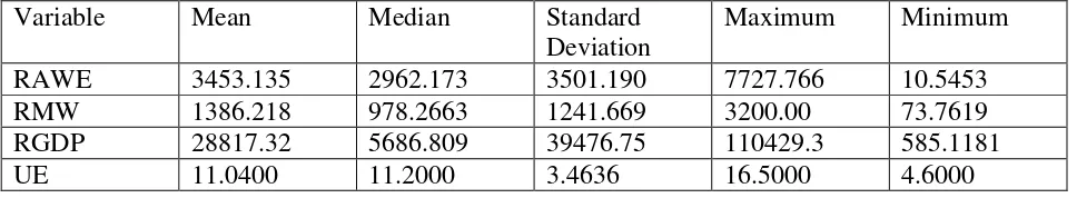
35 Table 3: Descriptive Statistics (Panel Data)
Variable Mean Median Standard Deviation
Maximum Minimum
RGPDUS 4517.079 860.6690 6278.405 17557.92 7.0562 RAWEUS 67.8389 39.2614 71.8022 208.1571 1.6868 RMWUS 39.0143 44.8730 15.6030 65.0492 11.7086 UE 11.0400 11.2000 3.4637 16.5000 4.6000
Table 4: Descriptive Statistics (Time Series Data)
Variable Mean Median Standard Deviation
Maximum Minimum
[image:36.612.66.550.275.364.2]36
Figure 1(i): KERNEL DENSITY PLOTS FOR TIME-SERIES DATA (JAMAICA)
.0000 .0005 .0010 .0015 .0020 .0025 .0030 .0035
200 300 400 500 600 700 800
RGDP
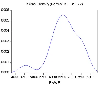
[image:37.612.84.419.125.398.2]37 Figure 1 (ii)
.0000 .0001 .0002 .0003 .0004 .0005 .0006
4000 4500 5000 5500 6000 6500 7000 7500 8000
RAWE
[image:38.612.85.413.117.404.2]38 Figure 1 (iii)
.00 .01 .02 .03 .04 .05 .06 .07 .08 .09
8 12 16 20 24 28
UE
[image:39.612.82.401.135.414.2]39 Figure 1 (iv)
.0000 .0001 .0002 .0003 .0004 .0005 .0006
500 1000 1500 2000 2500 3000 3500
RMW
[image:40.612.84.413.121.381.2]40
Figure 2 (i): KERNEL DENSITY GRAPHS FOR THE PANEL DATA
.000 .001 .002 .003 .004 .005 .006 .007
-40 0 40 80 120 160 200 240
RAWEUS
[image:41.612.84.408.124.399.2]41 Figure 2(ii)
.00000 .00002 .00004 .00006 .00008 .00010
-5000 0 5000 10000 15000 20000
RGDPUS
[image:42.612.81.420.99.396.2]42 Figure 2(iii)
i
The GMM and the TSLS methods are similar in that both make use of instrumental variables; however, the interpretation of tests of significance are somewhat different. TSLS uses the total number of observations multiplied by the TSLS R2 (this is the calculated test statistic for the overall model), this is compared with a chi-square distribution at 5% significance level with l – k degrees of freedom (l is the number of instruments and k is the number of parameters). If the tabled chi square value is less than the calculated value, the null hypothesis of exogeneity is failed to be accepted. A regression without a constant renders the coefficient of variation useless. In
contrast, The GMM test statistic for the model is T multiplied by the Hansen’s J-Statistic, if this statistic is less than
.000 .005 .010 .015 .020 .025 .030 .035
0 10 20 30 40 50 60 70
RMWUS
[image:43.612.84.407.90.385.2]43
the chi-square statistic at 5% significance level with l- k degrees of freedom, the null hypothesis cannot be