ISSN Online: 2333-9721 ISSN Print: 2333-9705
Properties of the Maximum Likelihood
Estimates and Bias Reduction for Logistic
Regression Model
Nuri H. Salem Badi
Mathematics Department, Faculty of Art and Science—Alabyar, University of Benghazi, Benghazi, Libya
Abstract
A frequent problem in estimating logistic regression models is a failure of the likelihood maximization algorithm to converge. Although popular and ex-tremely well established in bias correction for maximum likelihood estimates of the parameters for logistic regression, the behaviour and properties of the maximum likelihood method are less investigated. The main aim of this paper is to examine the behaviour and properties of the parameters estimates me-thods with reduction technique. We will focus on a method used a modified score function to reduce the bias of the maximum likelihood estimates. We also present new and interesting examples by simulation data with different cases of sample size and percentage of the probability of outcome variable.
Subject Areas
Applied Statistical Mathematics
Keywords
Logistic Regression Model, Maximum Likelihood Method, Convergence Problems, Bias Reduction Technique
1. Introduction
The logistic regression methods are often used to interpret the statistical analysis of dichotomous outcome variables. It is commonly applied procedure for describing the relationship between a binary outcome variable. The general method of estimating the logistic regression parameter is maximum likelihood (ML). In a very general sense the ML method yields values for the unknown parameters that maximize the probability of the observed set of data. The commonly problem with using ML method is convergence problem, which
How to cite this paper: Badi, N.H.S. (2017) Properties of the Maximum Likeli- hood Estimates and Bias Reduction for Logistic Regression Model. Open Access Li- brary Journal, 4: e3625.
https://doi.org/10.4236/oalib.1103625
Received: April 21, 2017 Accepted: May 21, 2017 Published: May 24, 2017
Copyright © 2017 by author and Open Access Library Inc.
This work is licensed under the Creative Commons Attribution International License (CC BY 4.0).
http://creativecommons.org/licenses/by/4.0/
occurs when the maximum likelihood estimates (MLE) do not exist. The subject of the assessment behaviour of MLE for logistic regression model is important, as the logistic model is widely used in medical statistics. Much work discusses on logistic regression model address converges problem like [1] or the bias reduction like [2][3]. Many assumptions and more details considered about the distribution of the coefficients estimated by MLE approach and bias reduction technique, and also for more application and effects of the sample size, see [4] [5]. However, the behavior and properties of bias correction methods are less investigated. A recent paper takes the bias correction technique proposed by [2] to achieve the MLE existing. In the present paper, it centers to evaluate the behavior and properties of the bias reduction method by simulated data with different sample sizes and parameters. The next section, explains the shape and fits the logistic regression model. Section 3 discusses clearly the ML convergence problem. Application on modified score function in logistic regression model will discuss in Section 4 and it illustrates special case of modified function to give two equations that are used to estimate the parameters. Section 5 investi- gates the asymptotic properties for logistic regression model with making compression between estimated parameters with ML method and reduction technique by simulated data. The discussion, conclusion and some general remarks about the results are in Section 6.
2. The Logistic Regression Model
The goal of a logistic regression analysis is to find the best fitting model to describe the relationship between an outcome and covariates where the outcome is dichotomous. [6] considered the logistic regression model is a member of the class of the generalized linear models. For more details of logistic model see [7] [8][9] also [10][11][12].
The Model
Suppose now yi~ binomial
(
mi,πi)
where y ii, =1, , n is a responsevariable. Suppose that yi∈
{
0,1, , mi}
and πi are related to a collection ofcovariates
(
x x
i1, , ,
i2x
ip)
according to the equation T1
log 1
p i
j ij i
j i
x x
π β β
π =
= =
−
∑
(1)We consider the special case mi=1 so yi ~ binomial 1,
(
πi)
where πi isthe probability of success for each i=1, , n. We also define T
i xi
η =β so that
( )
log1 i
i i
i
g π π η
π
= =
−
(2)
and
( )
( )
exp 1 exp i
i
i
η π
η
=
+ (3)
Here g
( )
. is called the logit link function and T 1p
i j j ijx xi
There are some other link functions which can also be used, instead of the logit link function such as the probit link function
( )
( )
1
η
= Φ−π
↔ = Φπ
η
and the complementary log-log link function
(
)
(
)
( )
log log 1
1 exp e
ηη
=
−
−
π
↔ = −
π
−
Fitting The Model
The logistic model when yi~ binomial
(
mi,πi)
with mi=1 can be fittedusing the method of maximum likelihood to estimate the parameters. The first step is to construct the likelihood function which is a function of the unknown parameters. we choose those values of the parameters that maximize this function. The probability function of the model is
( )
(
)
11
ii y
y
i i i
f y
=
π
−
π
− (4) where the likelihood function is(
)
(
)
1
| n |
i i i i
i
L
π
y f yπ
=
=
∏
(5)Since the observations are independent, the likelihood function is as follows:
(
)
(
)
11
| n yi 1 yi
i i i i
i
L
π
yπ
π
−=
=
∏
− (6)The maximum likelihood estimate of
β
is the value which maximizes thelikelihood function. In general the log likelihood function is easier to work with mathematically and is:
( ) (
) (
)
1 log 1 log 1
n
i i i i
i
l y
π
yπ
=
=
∑
+ − − (7)2.1. Special Case of the Logistic Model with Two Covariates
In this case the logistic regression model with two covariates, thus,
p
=
2
, with one the general mean. So, we have β0 and β1, such that( )
i i 0 1 ig π =η =β +β x (8)
where xi is now a scalar covariate and
(
)
(
0 0 11)
exp 1 exp
i i
i
x x
β β
π
β β
+ =
+ + (9)
Therefore we can write the log-likelihood function as:
(
0 1)
(
0 1)
(
0 1)
1
, n i i log 1 exp i
i
l
β β
yβ
β
xβ
β
x=
=
∑
+ − + + (10)To estimate the values of β0 and β1 we differentiate l
(
β β0, 1)
in terms of0
β and β1 respectively as:
(
)
(
0 1)
(
)
1 1
0 0 1
exp 1 exp
n n
i
i i i
i i i
x
l y y
x
β β π
β = β β =
+
∂ = − = −
(
)
(
)
(
0 1)
(
)
1 1
1 0 1
exp 1 exp
n i i n
i i i i i
i i i
x x
l y x y x
x
β
β
π
β
=β
β
=+
∂ = − = −
∂
∑
+ +∑
(12)Now we set
0
0
l
β
∂ =∂ and 1 0
l
β
∂ =∂ and so the maximum likelihood estimates
of β0 and
β
1 are the solution of the following equations1 1
n n
i i
i y i
π
= =
=
∑
∑
(13)and
1 1
n n
i i i i
i y x i x
π
= =
=
∑
∑
(14)and will be denoted as βˆ0 and βˆ1. We know that for the logistic regression the
last two equations are non linear in β0 and β1, and we need to use a
numerical method for their solution, such as Newton-Raphson method.
2.2. The Asymptotic Distribution of the (MLE)
The estimated parameters βˆ=
(
β βˆ ˆ0, 1)
′, have an asymptotic distribution whichis given by βˆ ~N
(
β,I( )
β −1)
where I
( )
β is Fisher’s information matrix defined as( )
2 2 2 0 1 0 2 2 21 0 1
l l I E l l β β β β
β β β
∂ ∂ ∂ ∂ ∂ = − ∂ ∂ ∂ ∂ ∂ (15)
where the matrix is evaluated at the MLE. For the logistic regression the estimated Fisher Information matrix can be writen as
( )
(
)
(
)
(
)
(
)
1 1
2
1 1
ˆ 1 ˆ ˆ 1 ˆ
ˆ
ˆ 1 ˆ ˆ 1 ˆ
n n
i i i i i
i i
n n
i i i i i i
i i
x I
x x
π π π π
β
π π π π
= = = = − − = − −
∑
∑
∑
∑
(16)where ˆ exp
( )
ˆ( )
ˆ 1 exp i η π η =+ and η βˆ= ˆ0+βˆ1xi. The variance of βˆ is approximated
defined by Var
( ) ( )
βˆ =I βˆ −1.3. Maximum Likelihood Convergence Problems
A problem occurs in estimating logistic regression models when the maximum likelihood estimates do not exist and one or more components of βˆ are infinite. The one case of the occurrence of this problem is when all of the observations have the same response. For example, suppose that mi=1 and
that all of the response variables equal zero i.e., 1
0
ni i=
y
=
∑
. In this case the log-likelihood function is(
0 1)
(
0 1)
1
, n log 1 exp i
i
l
β β
β
β
x=
Now differentiating l
(
β β0, 1)
in terms of β0 and β1 respectively andsetting equal to zero gives
(
)
(
0 1)
1 1 0 1
ˆ ˆ
exp
0
ˆ ˆ
1 exp
n n i
i
i i i
x x
β β
π
β β
= =
+
= =
+ +
∑
∑
(18)and
(
)
(
0 1)
1 1 0 1
ˆ ˆ
exp
0
ˆ ˆ
1 exp
n n i
i i i
i i i
x
x x
x
β β
π
β β
= =
+
= =
+ +
∑
∑
(19)The first equation has no solution because it is the sum of positive quantities and so cannot be equal to zero and satisfy the equation. To make this equation equal to zero we need to make β0 larger and negative i.e. tend to −∞.
However, if precisely one of the response variable equal 1, the result maximum likelihood equation become
1
1
n i i
π
==
∑
(20)1 1
n i i
i x x
π
==
∑
(21)where we have assumed the numbers such that y1 =1. Here the maximum
likelihood estimates is exist and the convergence of the MLE is achieved. Because the two previous equations are sum of positive quantities equal positive values. So as in first equation, if parameter is large and positive, then the sum is larger than one as well as if it is large and negative, then the sum is smaller than one and will not satisfy the equation, then we can find finite estimate of parameters which satisfy the equation.
4. Modified Score Function
Firth [2] proposed a method to reduce bias in MLE. The maximum likelihood convergence problem does not exist with the modified score function. The idea that extend and focus on two standard approaches have been extensively studied in the literature. The computationally-intensive jackknife method proposed by [13] [14]. The second approach simply substitutes βˆ for the unknown
β
in( )
bn β
. The point that discussed in case of small size sets of data, it is not uncommon that βˆ is infinite in some samples of logistic regression models [15][16]. We know that the maximum likelihood approach is dependent on the derivative the log-likelihood function as a solution to the score equation
( )
( )
0
l β U
β β
∂
= =
∂ (22)
[2] proposed that instead, we solve U*
( )
β =0, where the appropriatemodification to U
( )
β is:( )
( ) ( ) ( )
*
and the expected value of βˆ proposed by [3], is given by:
( )
ˆ( )
ˆ( )
1E β = +β b β +O n− (24)
where
( )
2 3
2 3
2 2
2
2
2
l l l
E E
b
l E
β β
β
β
β
∂ ∂ + ∂ ∂ ∂ ∂
=
∂
∂
The variance of βˆ is approximated defined by Var
( ) ( )
βˆ I βˆ −1.4.1. Modified Function with Logistic Regression Model
In this part we will apply the modified score function to simple logistic regression model. We know that the
O n
( )
−1 bias vector given in the form(
T)
1 Tb= X WX − X W
ξ
which proposed by [17]. HereW
ξ
has ith element1 2
i i
h
π
− and hi is the ith diagonal element of the hat matrix
(
)
11 2 T T 1 2.
H W X X WX= − X W
where
W diag
=
(
π
i(
1
−
π
i)
)
and X is the design matrix. Then, the modified score function is written as* T
U =U X Wξ− (25) In this case, the modified score function *
(
* *)
0
,
1U
=
U U
gives two equations(
)
* 0
1 2 1 0
n
i
i i i
i
h
U y h π
=
= + − + =
∑
(26)and
(
)
* 1
1 2 1 0
n
i
i i i i
i
h
U y h π x
=
= + − + =
∑
(27)These are used to estimate the parameters.
4.2. Special Case of Modified Function
For more evaluation, we will discuss the behaviour of the adjusted score function when all the observation have the same response i.e. 1
0
n i i=
y
=
∑
. As a special case, suppose we have one explanatory variable xi taking values 0 or 1. Beforewe calculate the adjusted score function, first calculate the form of hi which we
obtain from H. Here, hi is the diagonal element of the H matrix and is
(
)
(
2)
2 1 0
1 2
i i i i
i
X x X x X
h =π −π − +
∆ (28)
where 2
0 2 1
X X X
∆ = − , X0=n0 0π
(
1−π0)
+n1 1π(
1−π1)
, X1=n1 1π(
1−π1)
and X2=n1 1π
(
1−π1)
, where n0 and n1 are the number of observations of xequal to 0 and 1 respectively. Hence
(
)
(
)
0 0 1 1 1
0
1 n 1
h =π −π π −π
and
(
)
(
)
1 1 0 0 0
1
1 n 1
h =π −π π −π
∆ (30)
Therefore, when we set the adjusted score function
(
U U
*0,
1*)
=
0
with1
0
n i i=
y
=
∑
we have(
)
* 1 1 1 0 2 n ii i i
i
h
U h
π
x=
= − + =
∑
(31)This gives
(
)
1 1 1 1 0 2h h
π
− + =
(32)
and
(
1)
1 1 2 1 h h π =
+ (33)
Now,
(
)
* 0 1 1 0 2 n i i i i hU h
π
=
= − + =
∑
(34)and so
(
)
0(
)
1
1n2 1 1 1 1 0n2 0 1 0 0 0
h n h
π
h n hπ
− + + − + =
(35)
we get
(
0)
0 0 2 1 h h π =
+ (36)
Before calculate π0 and π1 we can consider the following way to calculate 0
h and h1. Let A n= 1 1π
(
1−π1)
and B n= 0 0π(
1−π0)
. Then, X0= +A B,1
X =A and X2=A, so, we can write ∆ as
(
)
(
)
2 2 2
0 2 1 1 1 1 1 0 0 1 0
X X X A AB A AB n
π
π
nπ
π
∆ = − = + − = = − − (37)
Therefore, h0 and h1 can be written as
(
)
(
)
(
)
(
)
0 0 1 1 1
0
0
1 1 1 0 0 0
1 1 1
1 1
n h
n
n n
π π π π
π π π π
− −
= =
− −
(38)
and
(
)
(
)
(
)
(
)
1 1 0 0 0
1
1
1 1 1 0 0 0
1 1 1
1 1
n h
n
n n
π π π π
π π π π
− −
= =
− −
(39)
Then, we obtain
(
0)
(
0)
(
)
0
0 0 0
1 1
2 1 2 1 1 2 1
h n
h n n
π = = =
+ + + (40)
and
(
1)
(
1)
(
)
1
1 1 1
1 1
2 1 2 1 1 2 1
h n
h n n
π = = =
As a result of this example with x=0,1 when
∑
ni=1y
=
0
, we can say that, the estimate of parameters are finite. The modified function works well and the problem of convergence does not exist.5. Simulation Study
The follow discussion are the simulation plan and the designs used in generating the data to identify the effect of sample size and proportion of events (the percentage of
y
=
1
ory
=
0
) on estimation of parameters. We will examine the precision of the estimation by calculating the variance of parameters obtained by simulation for the two approaches, MLE and Firth, and compare those withI
( )
β
−1evaluated at the known values of
β
. The simulation study is designed as follows:1) Thre sample sizes have been used n=40, n=120 and n=500.
2) For each sample size we choose xi as a draw from N
( )
0,1 . The x variablesare fixed at these values throughout the simulation.
3) We choose β0 and β1 to give three cases. Choose β =1 0.2 and adjust 0
β so that over the covariates pr
(
y=1)
is approximately (a) 0.5, (b) 0.1, (c)0.05.
4) For each sample size and set of parameter values we perform 100,000 simulation.
5) Two approaches are used to estimate the parameters, MLE and the bias- reduced estimator Firth.
5.1. Results and Discussion of Sample Size
n
= 500
The simulation reported the accuracy of the estimation of Var
( )
βˆ using the information matrix. We calculate Var( )
βˆ0 and Var( )
βˆ1 for the simulatedvalues of βˆ0, βˆ1 and also by evaluating I
( )
β at the known values ofβ
. Theresults in the Table 1, which shows the three cases of the proportion of
y
=
1
, achieved the convergence of likelihood maximization alogrithm.As can be seen in Table 1, VarβˆL Sim and VarβˆF Sim are the variance of
the parameters estimated by MLE and Firth method respectively. Ratio L and Ratio F denote the ratio of the variance estimated by MLE and Firth’s method, respectively. The results showed that, both the variance of the parameters calculated from the simulation and the variance calculated by evaluating the information matrix at the known values of
β
are almost the same. We notethat the ratio in the first case when pr
(
y=1)
is 0.5 appeared nearly close toone but in the second case and the last case the ratio appeared slightly larger than in the first case.
The variance of parameters calculated by Firth’s method were smaller than when calculated by MLE and the ratio in general was close to 1. Moreover, the bias (β βˆ -F ) was smaller.
5.2. Results and Discussion of Sample Size
n
= 120
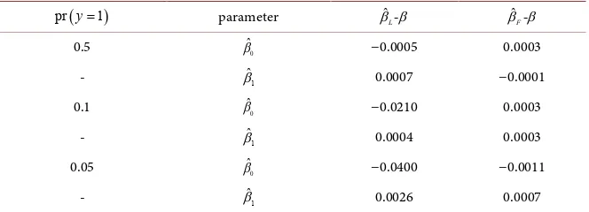
Table 1. Results of 100,000 simulations with sample size n = 500 and (0.5, 0.1, 0.05) propotion of y = 1.
(a)
(
)
pr y=1 parameter VarβˆL Sim VarβˆF Sim Varβˆ Inf Ratio L Ratio F
0.5 βˆ0 0.00804 0.00813 0.00809 0.99 1.005 - βˆ1 0.00869 0.00862 0.00858 1.01 1.04 0.1 βˆ0 0.02407 0.02359 0.02312 1.04 1.02 - βˆ1 0.02455 0.02439 0.02390 1.03 1.02 0.05 βˆ0 0.04938 0.04560 0.04411 1.12 1.03 - βˆ1 0.04725 0.04656 0.04525 1.04 1.03
The variance of the parameters estimated by MLE and Firth with (0.5, 0.1, 0.05) propotion of y = 1.
(b)
(
)
pr y=1 parameter β βˆ -L β βˆ -F
0.5 βˆ0 −0.0005 0.0003
- βˆ1 0.0007 −0.0001
0.1 βˆ0 −0.0210 0.0003
- βˆ1 0.0004 0.0003
0.05 βˆ0 −0.0400 −0.0011
- βˆ1 0.0026 0.0007
The bias value with (0.5, 0.1, 0.05) propotion of y = 1.
results of simulation are shown in Table 2. Maximum likelihood convergence problems occurred (when pr
(
y= =1)
0.05). Note that, there are many situationsin which the likelihood function has no maximum, in which case we say that the maximum likelihood estimate does not exist. Consider the simulation which generating the data set 100,000 times, in some cases the coefficients reach to infinite in the final iterations and so, we have not results of the estimation βˆ0
and βˆ1, that result in at which point the algorithm has not converged. In our
simulation we consider the cases that not achieved the converges algorithm. Here for only 99,806 (99%) of the data sets was it possible to obtain finite estimates of β0 and β1 converged. Moreover, the variance of the parameters
0
ˆ
β and βˆ1 is large. This is because even though convergence is achieved when
1
1
n i i=
y
=
∑
, There are some very large negative values of βˆ. In the other two cases of pr(
y=1) (
= 0.5,0.1)
we achieved ML convergence in every simulation.We note that the ratio is nearly one but is a bit high when compared with case of
500
n= . Firth’s approach showed reasonable results, all cases achieved the maximum likelihood convergence. Moreover, the ratio was better than MLE approach as well as the bias β βˆ -F .
5.3. Results and Discussion of Sample Size
n
= 40
We used the same analysis as in the previous cases with n=40. As can be seen
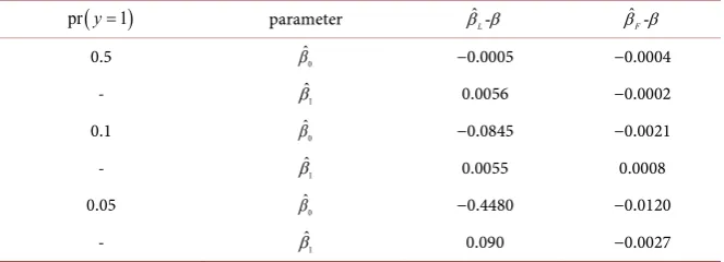
Table 2. Results of 100,000 simulations with sample size n = 120 and (0.5, 0.1, 0.05) propotion of y = 1.
(a)
(
)
pr y=1 parameter Varˆ
L
β Sim VarβˆF Sim Var Inf Ratio L Ratio F
0.5 βˆ0 0.034 0.0335 0.0337 1.04 0.99 - βˆ1 0.035 0.0331 0.0326 1.07 1.01 0.1 βˆ0 0.125 0.1037 0.0951 1.32 1.09 - βˆ1 0.105 0.0942 0.0885 1.27 1.06 0.05 βˆ0 230.94 0.2377 0.1811 - 1.31 - βˆ1 37.96 0.2003 0.1669 - 1.20
The variance of the parameters estimated by MLE and Firth with (0.5, 0.1, 0.05) propotion of y = 1.
(b)
(
)
pr y=1 parameter β βˆ -L β βˆ -F
0.5 βˆ0 −0.0005 −0.0004
- βˆ1 0.0056 −0.0002
0.1 βˆ0 −0.0845 −0.0021
- βˆ1 0.0055 0.0008
0.05 βˆ0 −0.4480 −0.0120
- βˆ1 0.090 −0.0027
The bias value with (0.5, 0.1, 0.05) propotion of y = 1.
Table 3. Results of 100,000 simulations with sample size n = 40 and (0.5, 0.1, 0.05) propotion of y = 1.
(a)
(
)
pr y=1 parameter VarβˆL Sim VarβˆF Sim Var Inf Ratio L Ratio F
0.5 βˆ0 0.12184 0.1076 0.10780 1.13 0.99 - βˆ1 0.14889 0.1222 0.11766 1.22 1.04 0.1 βˆ0 215.38 0.3702 0.29139 - 1.27 - βˆ1 81.22 0.3962 0.34304 - 1.16 0.05 βˆ0 820.47 0.5080 0.55184 - 0.92 - βˆ1 295.64 0.5936 0.65309 - 0.91
The variance of the parameters estimated by MLE and Firth with (0.5, 0.1, 0.05) propotion of y = 1.
(b)
(
)
pr y=1 parameter β βˆ -L β βˆ -F
0.5 βˆ0 0.0029 −0.0001
- βˆ1 0.0220 −0.0010
0.1 βˆ0 −1.2000 −0.0150
- βˆ1 0.3830 −0.014
0.05 βˆ0 −3.9900 0.0440
- βˆ1 1.288 −0.0940
[image:10.595.208.539.607.722.2]98,273 (98%) and 85,967 (86%) of data sets achieved ML convergence when
(
)
pr y=1 was (0.1, 0.05), respectively. Convergence was only achieved in every
simulation in the case of pr
(
y=1)
=0.5, where the ratio was nearly close to one, but is a bit high from previous cases. Moreover, we found the same problem as discussed in the case of n=120, in that the variance of the parameters βˆ0and βˆ1 is large. However, when we use Firth’s approach, all data sets achieved
M.L convergence. Moreover, the ratio was better than M.L.E approach as well as the bias β βˆ -F being smaller.
6. Conclusion
Attention has been directed in this work to determine the behaviour of the asymptotic estimation of parameters by two methods—MLE and bias reduction technique compared with the result of the information matrix. In fact in regular convergence problem the modified score function appeared appropriate behaviour, which denoted that the bias form may be removed from the MLE by reduction bias term. The asymptotic variance of the MLE may be appeared as strange behaviour, and the results shown variance of the parameters were large in some cases, even though convergence is achieved. It is denoted that there are some very large negative values of βˆ, as shown in results section. We can report that the small sample size and the value of pr
(
y=1)
have an effect onbehaviour estimation of parameters when using MLE. Clearly, we found conver- gence problem for some combinations of sample size and pr
(
y=1)
. Theapproach of Firth appeared a moderate results that the data sets in all cases of sample size and pr
(
y=1)
achieved ML convergence. Overall, we can considerthe bias reduction technique is worked well and has a moderate behaviour almost with all cases which have been investigated. Moreover, the convergence problem is not only effective on behaviour of the MLE, and although the convergence is achieved, the variance of the parameters estimates appeared large value.
References
[1] Cox, D.R. and Hinkley, D.V. (1974) Theoretical Statistics. Chapman and Hall, London.
[2] Firth, D. (1993) Bias Reduction of Maximum Likelihood Estimates. Biometrika, 80, 27-38. https://doi.org/10.1093/biomet/80.1.27
[3] Anderson, J.A. and Richardson, C. (1979) Logistic Discrimination and Bias Correc-tion in Maximum Likelihood EstimaCorrec-tion. Technometrics, 21, 71-78.
[4] McCullagh, P. (1986) The Conditional Distribution of Goodness-of-Fit Statistics for Discrete Data. Journal of the American Statistical Association, 81, 104-107. https://doi.org/10.1080/01621459.1986.10478244
[5] Shenton, L.R. and Bowman, K.O. (1977) Maximum Likelihood Estimation in Small Samples. Griffin’s Statistical Monograph No. 38, London.
[6] Nelder, J.A. and Wedderburn, R.W.M. (1972) Generalized Linear Models. Journal of the Royal Statistical Society, Series A, 135, 370-384.
[7] Dobson, A. (1990) An Introduction to Generalized Linear Models. Chapman and Hall, London.
[8] Dobson, A.J. and Barnett, A.G. (2008) An Introduction to Generalized Linear Mod-els. 3rd Edition, Chapman and Hall, New York.
[9] Kleinbaum, D.G. (1994) Logistic Regression: A Self-Learning Text. Springer-Verlag, New York. https://doi.org/10.1007/978-1-4757-4108-7
[10] Hilbe, J.M. (2009) Logistic Regression Model. Chapman and Hall, New York. [11] Hosmer, D.W. and Lemeshow, S. (2000) Applied Logistic Regression. Wiley, Chi-
chester. https://doi.org/10.1002/0471722146
[12] Hosmer, D., Lemeshow, S. and Sturdivant, R.X. (2013) Applied Logistic Regression. 3rd Edition, Wiley, Chichester. https://doi.org/10.1002/9781118548387
[13] Quenouille, M.H. (1949) Approximate Tests of Correlation in Time-Series. Journal of the Royal Statistical Society: Series B, 11, 68-84.
[14] Quenouille, M.H. (1956) Notes on Bias in Estimation. Biometrika, 43, 353-360. https://doi.org/10.1093/biomet/43.3-4.353
[15] Albert, A. and Anderson, J.A. (1984) On the Existence of Maximum Likelihood Es-timates in Logistic Regression Models. Biometrika, 71, 1-10.
https://doi.org/10.1093/biomet/71.1.1
[16] Clogg, C.C., Rubin, D.B., Schenker, N., Schultz, B. and Weidman, L. (1991) Multiple Imputation of Industry and Occupation Codes in Census Public-Use Samples Using Bayesian Logistic Regression. Journal of the American Statistical Association, 86, 68-78. https://doi.org/10.1080/01621459.1991.10475005
[17] McCullagh, P. and Nelder, J.A. (1989) Linear Models. 2nd Edition, Chapman and Hall, London.
Submit or recommend next manuscript to OALib Journal and we will pro-vide best service for you:
Publication frequency: Monthly
9 subject areas of science, technology and medicine Fair and rigorous peer-review system
Fast publication process
Article promotion in various social networking sites (LinkedIn, Facebook, Twitter, etc.)
Maximum dissemination of your research work