Forecasting Time Varying Correlation using the Dynamic Conditional Correlation (DCC) Model

(1)

Munich Personal RePEc Archive

Forecasting Time-Varying Correlation

using the Dynamic Conditional

Correlation (DCC) Model

Mapa, Dennis S. and Paz, Nino Joseph I. and Eustaquio,

John D. and Mindanao, Miguel Antonio C.

School of Statistics, University of the Philippines Diliman

2014

Online at

https://mpra.ub.uni-muenchen.de/55861/

(2)

Forecasting Time-Varying Correlation using the Dynamic Conditional Correlation (DCC) Model Dennis S. Mapa, Niño Joseph I. Paz, John D.Eustaquio and Miguel Antonio C. Mindanao

School of Statistics, University of the Philippines Diliman

ABSTRACT

Hedging strategies have become more and more complicated as assets being traded have become more interrelated to each other. Thus, the estimation of risks for optimal hedging does not involve only the quantification of individual volatilities but also include their pairwise correlations. Therefore a model to capture the dynamic relationships is necessary to estimate and forecast correlations of returns through time. Engle’s dynamic conditional correlation (DCC) model is compared with other models of correlation. Performance of the correlation models are evaluated in this paper using only the daily log returns of the closing prices of the Peso-Dollar Exchange Rate and Philippine Stock Exchange index. Ultimately, Engle’s DCC model is adopted because of its consistency with expectations. Though generally negative, correlation between these two returns is not really constant as the results indicated. The forecast evaluation of the models was divided into in-sample and out-of-sample forecast performance with short-term (i.e., 22-day, 60-day, and 125-day) and medium-term (250-day and 500-day) rolling window correlations, or realized correlations, as proxies for the actual correlation. Based on the root mean squared error and mean absolute error, the integrated DCC model showed optimal forecast performance for the in-sample correlation patterns while the mean-reverting DCC model had the most desirable forecast properties for dynamic long-run forecasts. Also, the Diebold-Mariano tests showed that the integrated DCC has greater predictive accuracy in terms of the 3-month realized correlations than the rest of the models.

(3)

1

I. Introduction

Correlations are vital inputs for many of the tasks of financial risk management. Forecasts of future correlations and volatilities are the basis of any pricing formula for financial instruments or strategy that would aid an investor or a company in mitigating unnecessary risks. Thus, it has been a tale of the tape to efficiently and accurately forecast financial correlations for risk planning and policy-making purposes. Several models have already been developed to capture the correlation pattern of financial time series. Some of the most common models are the constant conditional correlation model, the diagonal VECH model, and the diagonal BEKK model, which are multivariate GARCH methods readily estimated in latest versions of most software packages. However, Engle (2001) proposed a model that addresses the structural and empirical weaknesses of the latter models and attempts to accurately and parsimoniously pin down the dynamic pattern of the correlation which is why it is aptly name as the dynamic conditional correlation (DCC) model. This paper aims to assess the performance of the DCC model in forecasting the correlations between the returns of two Philippine financial series – the Philippine Stock Exchange Index (PSEi) and the nominal Peso-Dollar exchange rate– and see how the results compare with other correlation models.

Philippine Financial Markets

(4)

2

It is generally regarded that all risks should be avoided since it can cause much uncertainty and trouble in any financial arrangement. However, if the investor can precisely pinpoint the direction and magnitude of movements in price levels, say of the PSEi or the Peso-Dollar exchange rate, then the investor can make a position that can be rewarding for his or her part. However, this strategy takes on the risks of sudden changes in markets due to misguided expectations or a misspecification of a forecasting method. Moreover, it would be desirable for investors to enter into risky investments but be protected from the possible pitfalls at the same time.

Hedging Problem

One way that investors and institutions can manage the risks they’re entering is through hedging, that is entering into another transaction whose sensitivity to fluctuations in prices counterbalances the sensitivity of their main transaction to such variations. A common hedging strategy is optimization of portfolio allocation. This entails minimizing the variance of the portfolio as it measures the level of risk of a pool of investments. The variance of a given portfolio is a function of the individual variability of each investment and their correlations with each other. Another hedging strategy commonly employed is the use of derivatives. Derivatives are basically contracts that are valued based on the price of other assets. They protect the holder of the contract by giving a payoff once a stipulated event occurs, usually a significant drop of the price level relevant to the main transaction, at a specific point of time. This protection however, comes with a premium to be paid at the commencement of the derivative, thus this financial instrument are almost synonymous with insurance.

(5)

3

the investor was able to insure himself for the possible downfall. However, a seller determining a fair price for the quanto involves information on several financial parameters such as volatilities, interest rates, exchange rates, and most importantly, the correlation between the PSE index and the Peso-Dollar exchange rate.

Economics of Correlations

Movements in the levels of financial series such as the PSEi and the Peso-Dollar exchange rate are very much determined by internal and external news that are relevant to them. This news includes government policy implementations, interventions in markets, inside information, and recessionary movements. Prices of assets constantly change in response to news and in anticipation of future performance. Moreover, if news affecting both assets are correlated, then the prices of these assets will also be correlated. Then, both the volatilities of and correlations between asset returns or prices will depend on the information to update their distribution (Samuelson, 1965). Because of the existence of this correlation, one can generally dictate how the price or return of an asset will move based on the movement of the other asset. However, the nature of the news that affect both assets also vary across time. Thus, it is proper to think that the correlations between these assets are also varying across time. It should also be noted that forward-looking correlations are considered more important for an investor as this will dictate how the investment should be structured so that expected future payoffs will be realized. Thus, it might be of advantageous to investors if accurate long-term correlations could be forecasted so that proper strategies can be employed.

(6)

4

Forecasting Correlations

In order to quantitatively capture the time-varying correlations between asset returns, several statistical models have been proposed various literatures. First and foremost, the parameters of interest are denoted as:

= | = ℎ , , ℎ , , ℎ , , ℎ , ,

the conditional covariance of two asset returns at time t

= , = the conditional correlation matrix of two asset returns at time t

The Constant Conditional Correlation model (Bollerslev, 1990) is a class of multivariate GARCH models which restricts the correlation matrix to be time invariant such that =

. Though the estimation is simple, one major drawback is that nothing much can be learned about the dynamics of the correlations while assuming they are constant, though some studies have pointed out a constant correlation pattern in some short-term periods. A more popular class of multivariate GARCH models is the diagonal multivariate GARCH or diagonal vector GARCH (diagonal VECH) which formulates the , element of the covariance matrix as the product of the prior and returns (Bollerslev, Engle, & Wooldridge, 1988). The first-order diagonal VECH model is given by:

ℎ, , = , + , , + ℎ, ,

However, the diagonal VECH model does not guarantee the positive definiteness of the resulting covariance matrices. The diagonal vector GARCH model was eventually modified to guarantee positive semi-definiteness of the covariance matrices by imposing a simple restriction for all the ’s to be the same and all the ’s to be the same, and requires that the matrix containing the elements _, to be positive definite. The model is called the diagonal BEKK vector GARCH model (Engle & Kroner, 1995) and it is given by:

(7)

5

It should be noted that for the diagonal VECH and diagonal BEKK models, the model specifies the dynamic pattern of the covariances, not the correlations, though they can be computed as an ad hoc procedure.

A model that directly estimates the conditional correlation is the dynamic conditional correlation model (Engle, 2002).This model formulates the volatilities of returns in one set of equations and the correlations between them in another set thus, treating them as independent stochastic processes, entailing more flexibility and different parameterizations. From the Monte Carlo simulations and real data context applications of the DCC model, it yielded the smallest mean absolute error among the vector GARCH and vector BEKK models, pinning much promise as to the quality of the results and simplicity of the method.

Many authors have used the DCC model to investigate the correlations of several macroeconomic variables. Bautista (2003) used the model to analyze the dynamic relationship between interest rate and exchange rate in the Philippines and saw that the correlations are mainly due to the effects of policies to exogenous events. Also, Vargas (2008) used a DCC model with an exogenous predictor to determine the key drivers of correlations between equity returns and exchange rate in select countries in Europe. Results show that interest rate differentials and capital flows were significant in explaining correlations between equity returns and exchange rate.

Significance and Limitations of the Study

One of the major motivations of this paper is that the correlations between assets are not constant through time. Testing data for constant correlation has proven to be a dilemma, as testing for dynamic correlation with data that have time-varying volatilities can result in misleading conclusions and lead to rejecting constant correlation when it is true due to incorrectly specified volatility models. This test only requires a consistent estimate of the constant conditional correlation, and can be implemented using a vector autoregression.

(8)

6

Due to the lack of access to previous data because the Manila Stock Exchange started the computerization of its operations and production of a One Price-One Market Exchange only in 1994 and fully implementing it during the third quarter of 2006, the researchers used the PSEi data from 2000-2010 to acquire a sufficient number of data points in a time series analysis.

Descriptive Analysis of Data

Daily data of the Philippine stock exchange index closing price and the Peso-Dollar exchange rate were used in the analysis. The PSEi data was obtained from Yahoo! Finance as provided by Commodity Systems, Inc., while the exchange rate data was taken from the Bangko Sentral ng Pilipinas.

Both time series were cleaned to have matching dates, which range from July 2, 1997 to February 26, 2010. The result is an irregular time series with 3,116 observations. However, the estimation period started from January 3, 2000 because of the irregular patterns of the series during the 1998 Asian crisis and so these observations were excluded from the analysis, leaving 2213 observations.

The analysis of the models was divided into in-sample and out-of-sample. The data that was used for the in-sample was from January 3, 2000 to December 24, 2008 while the out-of-sample consisted of the data from January 5, 2009 to February 26, 2010.

(9)

7

Government response to the crisis. The exchange rate also exhibited volatility with the Peso depreciating by 16.6 percent between March 1, 2008 and November 30, 2008 after appreciating by 39 percent against the US dollar between September 20, 2005 and February 29, 2008. Between July 2008 and January 2009—which is the relevant period for monitoring the immediate impact of the financial crisis—the Peso depreciated by only 3. Similar to stock prices the Peso was one of the currencies least affected by the crisis. Much could be learned from the model due to this partitioning of the data. This could also assess the adequacy of the model if the results from the forecasted out-of-sample jive with the general trend of the correlations.

The Dynamic Conditional Correlation Model

The DCC was used to model the time-varying correlations between the returns of the PSEi and the exchange rate. This model is commonly used to understand changes in correlations in asset returns by treating them as random processes. In this model, the correlation estimates are updated every time new information on volatility-adjusted returns arrives (Engle, 2002).

The first-difference of the logarithm of the prices of each asset was taken to extract the log returns of the PSEi and exchange rate. The DCC model requires the standardized residuals from the mean-variance specification of each return series. For stationary return series, the autoregressive moving average (ARMA) models can be used to model the mean while the generalized autoregressive conditional heteroskedasticity (GARCH) models can be used to capture the time-varying volatilities of each return series. To check whether there is a leverage effect on the volatilities of either series, a Threshold GARCH (TGARCH) model can be estimated. But first, stationarity of the return series should be tested using the Dickey-Fuller GLS (ERS) test of unit root before proceeding to the joint estimation of the ARMA-GARCH models.

After the estimation of the mean variance specification, the standardized residualof the ith

asset at time t is given by the formula:

, = , − ̂,

(10)

8

where _, is the actual return, ̂_, is the estimated mean return using the ARMA model, and ℎ_, is the estimated conditional variance using the GARCH model. The elements of the standardized residual vector,# for both the series is given by _, and _, .

For this study, two versions of the DCC model are used. Under the assumption that the changes in the correlations are mean-reverting and temporary, the mean-reverting DCC model is employed. First, a matrix Qt, called the quasi-correlation matrix, is postulated by the following

specification:

$ = % + # #& _{+ $}

To save up on the parameters in estimating the intercept matrix, correlation targeting is used to estimate the intercept parameters. The intercept estimate using correlation targeting is given by:

%' = 1 − − ), ) =_{+ , # #}1 &

-.

The new form of the mean-reverting DCC model is then given by: $ = ) + # #& _{− ) + $} _{− )}

It is guaranteed to be positive definite as long as the initial parameters α and β are all positive and that α + β< 1.

The integrated DCC model on the other hand assumes that the quasi-correlation matrix has a unit root process that is, the process has no tendency to revert to an unconditional value and is useful in modelling correlations that have structural breaks and are unlikely to be reversed. The specification of the quasi-correlation process under the integrated DCC model is given by:

$ = /# #& _{+ 1 − / $}

(11)

9

= diag4$ 5 67$ diag4$ 5 67

In summary, the estimation of the parameters of the DCC models was done by utilizing a two-step estimator. Since the log-likelihood for multiple series can be expressed as the sum of the log-likelihood of the variance parameters and the log-likelihood of the correlation parameters, the first step of the estimation was done by maximizing the variance part of the likelihood function which is taken care of by the ARMA-GARCH estimation. The standardized residuals were then obtained from the first step and the log-likelihood of the correlation parameters was maximized by the estimation of the DCC specification.

Correlation Proxy

To evaluate the forecast performance of the correlation models, several rolling window correlations were computed as proxy for the true correlations. The number of observations used in the rolling windows was based on common maturity terms of derivative contracts involving correlations, which include 1-month, 3-month, 6-months, 1-year, and 2-year terms. The correlations used to settle these contracts, which are called realized correlations, are basically computed using the daily log returns of the assets for the entire term of the contract. Thus, the computed 22-day, 60-day, 125-day, 250-day, and 500-day rolling window correlations which are used as proxy for the true correlation can be also called the 1-month, 3-month, 6-month, 1-year, and 2-year realized correlations. It should be noted however that these rolling correlations do not necessarily reflect the true value of the actual correlation at a specific day since it can only be computed from intraday data and that the rolling correlations are computed from data spanning several months. The rolling correlations, however, are utilized to observe the general trends and patterns of the actual correlation levels across time in the sense that a good correlation model should efficiently capture the dynamic movements of these proxy correlations.

Results and Discussion

Descriptive Analysis

(12)

10

and bearish periods on 2000 to 2002 and 2007 to 2009. For the earlier periods, the decline of the PSEi is subsequent to the effects of the tech bubble burst in the US. After 2002, a prolonged rebound can be seen as the PSEi rises until 2007 as the US housing bubble burst begins. The decline until 2008 shows its adverse effect to the local economy but 2009 shows signs of recovery as the PSEi levels begin to rise again. A strong evidence of a generally negative correlation is plausible as bullish stock market movements are generally accompanied by appreciative movements in the Peso with respect to the Dollar with the possible exception of the periods from early 2003 to 2004. Taking the viewpoint of Cappielo and De Santis’ uncovered equity return parity condition, the co-movement of the Peso-Dollar exchange rate and PSE index from this period suggests that the Philippines had higher expected equity returns than that of the US during this time which might be coupled to a positive local economy outlook while the US is recovering from the 2000 crisis. Also, the last three quarters of 2007 show both series being positively correlated once again as they both drop steadily. This might be attributed to the adverse effect of the housing bubble burst in the US economy, which caused the depreciation of the Dollar, while the crisis affects the global equity markets.

Moreover, Figure 1b shows the time plot of the log returns for both assets by using the dlog1 transformation. The returns of both assets appear to be stationary but volatility clustering and outliers are evident especially during the end of recessionary periods.

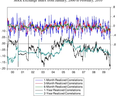
The sample correlation coefficients between the two daily log return series using moving windows of 22 days (i.e., 1 month), 60 days (i.e., 3 months), 125 days (i.e., 6 months), 250 days (i.e., 1 year), and 500 days (i.e., 2 years) are shown in Figure 2. The right and left axis of the graph show the short- (i.e., 1, 3, and 6 months) and medium-term (i.e., 1 and 2 years) moving correlations respectively. It is evident that the correlation changes over time and appears to be decreasing in the most recent periods as the economy recovers from the global financial crisis. The five correlation curves in Figure 2 look quite different from each other. The medium-term correlations are much smoother and easier to interpret over the short-term correlations. The monthly correlations have a great deal of volatility which looks like noise while the 3-month and 6-month correlations appear less fluctuating. However, the medium-term correlations do not

1

dlog(Pt)= log(Pt) – log(Pt-1) ≈ (Pt – Pt-1) / Pt-1, where Pt is the price of the asset at time t and log() is the natural

(13)

11

capture the actual movements since the over-all pattern is most evident. There are no statistical criteria in choosing between these measures thus, in comparing the results of the correlation forecasting models, all of these five measures will be used as points of comparison.

Figures 3a and 3b show the histogram and summary statistics of the prices and log returns respectively of the Peso-Dollar exchange rate and PSEi for both in- and out-of-sample periods. For the in-sample, the levels of the exchange rate and composite index are skewed to the left (Sk=-0.65) and right (Sk=0.89) respectively while the out-of-sample observations exhibit a more symmetric distribution (Sk=-0.24) for the exchange rate and a multi-modal distribution for the index. On the other hand, the distribution of the in-sample log returns for both series are generally asymmetric (Sk=-5.92 for exchange rate returns, Sk=0.58 for PSEi returns) and with excessive kurtosis (K=145.59 and K=19.71) which suggests non-constant conditional volatilities. The out-of-sample log returns for both series are more platykurtic (K=2.70 and K=4.11) and the Jarque-Bera test suggests that the out-of-sample returns for the Peso-Dollar exchange rate are normally distributed (test statistic=1.54, p=0.4623).

Univariate Analysis

The model building process for the mean-variance specification of the Peso-Dollar exchange rate and PSE index log returns will only consider the in-sample observations as the estimation sample. Tables 1a and 1b show the results of the Dickey-Fuller GLS (ERS) test for unit root for the log returns of the Peso-Dollar exchange rate and PSEi respectively. The test equations for the GLS detrended residuals of both log returns all have significant coefficients while the Elliott-Rothenberg-Stock DF-GLS test statistics (i.e., -9.34 and -36.82 for exchange rate and PSEi returns respectively) are both less than the critical values at 1% level of significance (i.e., -3.48). Thus, there is sufficient evidence to conclude that the log returns for both series are stationary2. This result would enable the de-GARCHING process of the DCC model estimation to allow for the modelling of the mean and variance processes with common models such as the ARMA and GARCH respectively.

The Univariate Box and Jenkins model building procedure was done to separately capture the mean and variance processes for each return series. Tables 2a and 2b show the final estimation output for the fitted models.

2

(14)

12

For the log returns of the Peso-Dollar exchange rate, an ARMA(1,3)-TGARCH(1,1) with conditional standardized Student-t (df=6.74) innovations was postulated after analyzing the sample partial autocorrelation function at different lag intervals of the log returns and squared log returns of the exchange rate while refining the equations by adding and dropping autoregressive (AR), moving average (MA), and volatility threshold terms until all the coefficients become significant at the 10% level. The joint estimation results are summarized in Table 2a. The model suggests that the log returns of the Peso-Dollar exchange rate are serially correlated because of the significant AR and MA terms and that its conditional volatility is not constant through time. Because the threshold term (-0.072) is significant, there is sufficient evidence that the effect of negative returns on future volatility is higher compared to positive returns, a phenomenon known as a leverage effect.

The same model building process was done for the log returns of the PSEi which is summarized in Table 2b. An AR(1)-TGARCH(1,1) with conditional standardized Student-t (df=5.12) innovations was jointly estimated as the final model. As with the log returns of the Peso-Dollar exchange rate, the log returns of the composite index exhibit dynamic persistence and serial correlations among returns while having time-varying volatilities with positive leverage effects (0.115).

After capturing the mean and the variance processes, the standardized residuals were obtained for both return series which would serve as the input series in the estimation of the correlation models.

In-Sample Performance

(15)

13

The initial values of alpha (0.05) and beta (0.86) where chosen since these values maximized the log-likelihood function. To see whether the estimation results are robust in terms of the initial values used, several runs of the maximum likelihood estimation were done while varying the initial values of alpha and beta and imposing the condition that their sum should be less than 1 to ensure positive definiteness of the resulting correlation matrices. The contour plots of the log-likelihood and estimated coefficients are shown in Figure 4. From Figure 4a, it can be seen that the maximum likelihood was achieved for the lower alpha and higher beta values, specifically at 0.05 and 0.86 with a log-likelihood of -2299.238. Changing the initial values also has an effect on the estimated alpha and beta coefficients, as evident from Figures 4b and 4c.

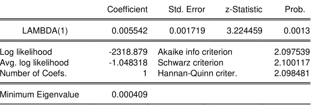
For the integrated dynamic conditional correlation model, the quasi-correlation estimation results are summarized in Table 3b. Unlike the mean-reverting DCC, the integrated DCC has only one parameter to be estimated. The initial value of 0.01 for lambda of the maximum likelihood estimation was chosen in the same manner as that for the mean-reverting DCC. A plot of the initial values of lambda with the log-likelihood and the estimated lambda coefficients appears in Figure 5. The graph shows that the log-likelihood achieves its highest value (-2318.879) for the smallest initial value of lambda (0.01) while the absolute log-likelihood exponentially increases as the initial value increases. The estimated lambda coefficient of 0.005542 (z-statistic=3.224, p=0.0013) is significantly different from zero which indicates a substantial persistence of the correlations from the unconditional level.

It should be noted that although convergence was not achieved for both mean-reverting and integrated DCC, Engle and Sheppard (2001) used only one iteration for the maximum likelihood estimation of the parameters since there is no guarantee that increasing the number of iterations would increase the log-likelihood function.

(16)

14

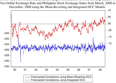
DCC model. However, the range of fluctuations were less pronounced in the mean-reverting model since the forecasted correlations for the period shown were as low as approximately -0.03 and as high as -0.022 while the forecasts of the integrated DCC model ranged from -0.022 to as high as 0.08. For both models, the long-run correlation between the log returns is generally negative which is consistent with literature as a high PSE index return and low exchange rate return is indicative of a healthy economy. However, there are some positive correlations forecasted in 2005 and 2008 from the integrated DCC model due to the co-movements of both Peso-Dollar exchange rate and PSEi in the months leading to these years.

For comparison purposes, several multivariate GARCH models such as the constant conditional correlation, diagonal VECH, and diagonal BEKK models were also estimated, the results of which are summarized in Table 4. As in the DCC models, the standardized residuals for both the log returns of the Peso-Dollar exchange rate and PSEi with zero mean specifications were used as the input series for the estimation of the multivariate GARCH models.

Figure 7a shows the correlation estimates from the multivariate GARCH models with those from the DCC models. Once again, the start-up problem of the integrated DCC model is distorting its overall pattern thus, Figure 7b shows the forecasted correlations once more using the truncated sample. The top part of the graph shows the forecasted correlations from the integrated DCC and diagonal VECH models which show fluctuations near the zero line, although the integrated DCC correlation forecasts are more persistent while the diagonal VECH forecasts are more volatile perhaps due to the non-positive definiteness of the forecasted correlation matrices inherent in the model itself. The bottom part of the graph shows the forecasts using the mean-reverting DCC, CCC, and diagonal BEKK models. The CCC fails to capture any dynamic pattern while being above the unconditional level of the diagonal BEKK and mean-reverting DCC estimates. The diagonal BEKK estimates are also volatile around the same level as the diagonal VECH estimates but have less extreme forecasts.

(17)

15

patterns from the realized correlations. To closely examine the trends of the forecasts, they were also compared to the medium-term realized correlations, as shown in Figure 9, since they have smoother shapes and have lesser fluctuations. From Figure 9b-1, the integrated DCC forecasts for the earlier months were problematic since they were very different but soon recovered, as shown in Figure 9b-2, as it closely follows the trend of the 1-year and 2-year realized correlations. As in Figure 8, the other models failed to capture the persistent pattern of the medium-term realized correlations.

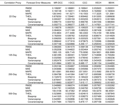
To evaluate the performance of the models in estimating the correlations, forecast error measures such as the root mean squared error, mean absolute error, mean absolute percentage error, Theil inequality coefficient, and the bias, variance, and covariance proportions of the mean squared forecast error are computed for each model as compared to the different realized correlations, which is summarized in Table 5. In comparing forecasts of the same series across different models, the RMSE and MAE are used since these statistics depend on the scale of the dependent variable. From the table, it can be seen that the integrated DCC model yielded the lowest RMSE for the short-term realized correlations while the mean-reverting DCC model is the lowest for the medium-term realized correlations. However, the integrated DCC model yielded the lowest MAE for all the realized correlations. These results are also evident in the plot of the rolling window used in the computation of the realized correlation versus the different forecast error measures for each model, as shown in Figure 10. The integrated DCC model performed best in terms of RMSE for the short-term correlations but performed the worst for medium-term correlations. On the other hand, the integrated DCC model uniformly had the lowest MAE for all rolling window values. This might be attributed to the wild forecasts that the integrated DCC produced during the start-up months and that the RMSE exaggerates its effect since it is a squared error measure unlike the MAE which is an absolute error measure. Thus, it can be said that the integrated DCC model is the model of choice for capturing the patterns in the in-sample correlations between the log returns of the Peso-Dollar exchange rate and PSE index due to its appealing empirical forecast properties.

Out-of-Sample Performance

(18)

16

Rolling Sample Forecasts

Figure 11 shows the 1-day, 2-day, 3-day, 4-day, and 5-day ahead correlation estimates from the DCC and multivariate GARCH models. There is not much difference with these graphs in terms of the forecast horizon since they are closely spaced with each other. Among the models, the integrated DCC model generated a different forecast pattern which is generally declining while the rest of the models still fluctuate around an unconditional level.

The 1-day ahead forecasted correlations from all the models are then compared to the short-term realized correlations which are shown in Figure 12. As in the in-sample results, the integrated DCC model is the only model that closely captured the trend of the declining realized short-term correlations though it doesn’t capture its specific movements. The forecasts of other models were still relatively level and do not reflect the declining correlations. These 1-day ahead forecasts were also compared with the medium-term realized correlations in Figure 13. Once again, the integrated DCC model dominated the rest in following the downward trend of the correlations.

To evaluate the performance of the models in estimating the correlations, forecast error measures as in the in-sample analysis were also computed for each model as compared to the different realized correlations and forecast horizons, which is summarized in Table 6. It can be seen that for the 1-month and 2-month realized correlations, the integrated DCC has the lowest RMSE and MAE across all forecast horizons. On the other hand, the mean-reverting DCC has the lowest RMSE and MAE for the 2-year realized correlations. For the 6-month and 1-year realized correlations, the integrated DCC has the lowest RMSE while the mean-reverting DCC has the lowest MAE.

These results are also evident in the plot of the rolling window used in the computation of the realized correlation versus the different forecast error measures of the 1-day ahead forecasts for each model, as shown in Figure 14. In terms of the RMSE, the integrated DCC model was the lowest for up to a 300-day rolling window and then the mean-reverting DCC became the lowest thereafter. For the MAE, the integrated DCC model performed best just before the 100-day rolling window and the mean-reverting DCC model then performed best for rolling windows greater than 100 days.

(19)

17

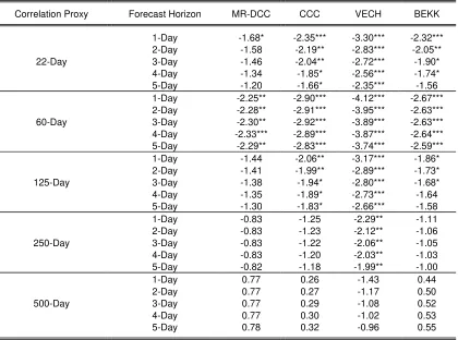
realized correlations. To formally test the predictive accuracy of the DCC model, say the integrated DCC model, several Diebold-Mariano tests using the squared error loss function were done to test whether the integrated DCC model significantly outperforms the other models in forecasting the realized correlations across the different rolling windows and forecast horizons. The results are summarized in Table 7. The Diebold-Mariano test statistics are approximately normally distributed with mean zero and variance one such that a left-tailed test would reject the null hypothesis of equal predictive accuracy if the test statistic is less than -2.32 at the 1% level of significance in favour of the alternative hypothesis that the integrated DCC model has a better predictive accuracy than the other models. The Diebold-Mariano tests results show that there is sufficient evidence to conclude that the integrated DCC model has a significantly greater predictive accuracy in forecasting the 3-month realized correlation across all forecast horizons and other models at 10% level of significance since the test statistics are all less than 1.645. However, the same conclusions cannot be said for the other realized correlations as proxies. In the case of the mean-reverting DCC model, if the alternative hypothesis is reversed such that a right-tailed test rejects the null hypothesis at the 10% level of significance for test statistics greater than 1.645. The table shows that the mean-reverting DCC has the same predictive accuracy across all forecast horizons than the integrated DCC since all the Diebold-Mariano test statistics are all less than 1.645 if the 2-year realized correlations are used as proxy.

(20)

18

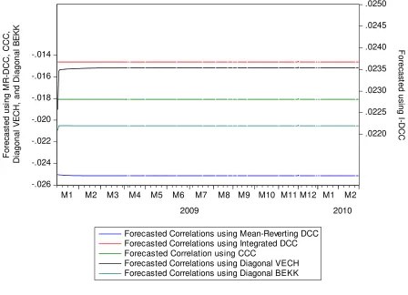
Dynamic Forecasts

For the long-run forecasts of correlations, Figure 15 shows the dynamic out-of-sample forecasts of the five models which are estimated using only the data from the in-sample. Since the coefficients of the integrated DCC model add up to 1, the best forecast of the correlation for all horizons is the forecasted correlation 1-day ahead of the in-sample. Thus, the dynamic forecasted correlations for the integrated DCC model are constant at the onset. But unlike the dynamic forecast of the CCC which is also constant, the integrated DCC forecast is pegged at the 1-day ahead forecast while the CCC forecast reflects the estimated long-run constant correlation. This is especially true for the other mean-reverting models such as the mean-reverting DCC, diagonal VECH, and diagonal BEKK since their dynamic forecasts for further horizons will eventually be constant at the estimated unconditional mean correlation. It can also be seen that for the mean-reverting DCC, diagonal VECH, and diagonal BEKK, the dynamic forecasts continue to change for as long as 5 days ahead before settling at a fixed value.

The forecasted correlations using dynamic forecasting are also compared with the short- and medium-term realized correlations in Figures 16 and 17. Because of the declining pattern of the realized correlations in the out-of-sample, all the models overestimated the correlation patterns but the mean-reverting DCC dynamic forecasts were the one closest to the average level of the realized forecasts.

Table 8 shows the forecast error measures as also computed in the in-sample and rolling sample forecast analysis in each model as compared to the different realized correlations to evaluate the performance of the models in estimating the correlations. The statistics indicate that the mean-reverting DCC model has the lowest RMSE and MAE across all realized correlations in terms of its dynamic correlation forecasts.

(21)

19

Based on the results of the forecast error measures, there is evidence to say that the mean-reverting DCC model is the optimal model in dynamically forecasting the out-of-sample correlation level for the log returns of the Peso-Dollar exchange rate and PSE index.

Conclusions

An understanding in the nature and scope of correlations between the Peso-Dollar exchange rate and PSEi returns is important in the estimation of risks for optimal hedging since it only does not involve only the quantification of individual volatilities but also include their pairwise correlations; as well as perceiving some ways to respond to the challenges in the economy. The dynamic conditional correlation model was used to estimate the correlation between these two returns. By employing both the mean-reverting and integrated DCC model, the results in this paper show that the correlation between the two returns is generally negative and is not really constant, but actually time-varying which is in accordance to the results of economic theories. The DCC models also produced more preferable results as to its flexibility, simplicity, and coherence with literature against other correlation models. Fluctuations in the correlations were caused by news affecting both the foreign exchange and equity markets. The integrated DCC model showed optimal forecast performance for the in-sample correlation patterns and rolling-sample forecasts of 1-day to 5-day horizons in terms of short-term realized correlations. On the other hand, the mean-reverting DCC model had the most desirable forecast properties for dynamic long-run forecasts and 1-day to 5-day rolling sample forecasts in terms of medium-term realized correlations. In terms of the short-run forecasting performance, the integrated DCC model was significantly higher in predictive accuracy than the other models using only the 3-month realized correlations as proxy.

Directions for Further Research

(22)

20

becomingly readily available, further forecast evaluation of the DCC models in this paper should be extended to include daily realized correlations as the basis of comparison and see whether the model can efficiently forecast them.

Acknowledgments

(23)

21 References

Aquino, R. Q. (2005). Exchange Rate Risk and Philippine Stock Returns: Before and After the Asian Financial Crisis. Applied Financial Economics, 15(11), 765-771.

Bautista, C. C. (2003). Interest Rate-Exchange Rate Dynamics in the Philippines: A DCC Analysis. Applied Economics Letters, 10, 107-111.

Bollerslev, T. (1990). Modelling the Coherence in Short-run Nominal Exchange Rates: A Multivariate Generalized ARCH Model. Review of Economics and Statistics, 69, 498-505.

Bollerslev, T., Engle, R. F., & Wooldridge, J. M. (1988). A Capital Asset Pricing Model with Time Varying Covariances. Journal of Political Economy, 96, 116-31.

Cappiello, L., & De Santis, R. A. (2005, September). Explaining Exchange Rate Dynamics: The Uncovered Equity Return Parity Condition. European Central Bank Working Paper Series.

Engle, R. (2009). Anticipating Correlations. Princeton, New Jersey: Princeton University Press. Engle, R. F. (2002). Dynamic Conditional Correlation: A Simple Class of Multivariate

Generalized Autoregressive Conditional Heteroskedasticity Models. Journal of Business and Economic Statistics, 20, 339-350.

(24)

22

[image:24.595.123.476.185.423.2]

Abridged Appendix: Figures and Tables

Figure 1a. Time Plot of the Closing Daily Prices of the Philippine Stock Exchange Index and Peso-Dollar Exchange Rate from January, 2000 to February, 2010

Figure 1b. Time Plot of the Log Returns of the Peso-Dollar Exchange Rate and Philippine Stock Exchange Index from January, 2000 to February, 2010

36 40 44 48 52 56 60

0 1,000 2,000 3,000 4,000

00 01 02 03 04 05 06 07 08 09

Peso-Dollar Exchange Rate Philippine Stock Exchange Index

-.12 -.08 -.04 .00 .04 .08

-.2 -.1 .0 .1 .2

00 01 02 03 04 05 06 07 08 09

[image:24.595.120.476.473.706.2]

(25)

[image:25.595.111.488.152.462.2]

23

Figure 2. Time Plot of the 22-Day (1-Month), 60-Day (3-Month), 125-Day (6-Month), 250-Day (1-Year), and 500-Day (2-Year) Realized Correlations between the

Log Returns of the Peso-Dollar Exchange Rate and Philippine Stock Exchange Index from January, 2000 to February, 2010

-.20 -.15 -.10 -.05 .00 .05 .10

-.8 -.4 .0 .4 .8

00 01 02 03 04 05 06 07 08 09

(26)

[image:26.595.72.412.290.442.2]

24

Table 3a. Estimated Parameters of the Mean-Reverting DCC Model between the Log Returns of Peso-Dollar Exchange Rate and the Log Returns of Philippine Stock Exchange Index with an

ARMA-TGARCH Specification LogL: MR_DCC

Method: Maximum Likelihood (BHHH) Sample: 1/04/2000 12/24/2008 Included observations: 2212 Evaluation order: By observation

Estimation settings: tol= 1.0e-05, derivs=accurate numeric Initial Values: ALPHA(1)=0.05000, BETA(1)=0.86000 Convergence not achieved after 1 iteration

Q = (1 - ALPHA(1) - BETA(1))*R + ALPHA(1)*RESID(-1)*RESID(-1)' + BETA(1)*Q(-1)

Coefficient Std. Error z-Statistic Prob.

R(1,1) 1.012139 -- -- -- R(1,2) -0.026112 -- -- -- R(2,2) 1.066428 -- -- -- ALPHA(1) 0.000386 0.012565 0.030715 0.9755

BETA(1) 0.854088 0.048812 17.49752 0.0000

Log likelihood -2299.238 Akaike info criterion 2.080686 Avg. log likelihood -1.039439 Schwarz criterion 2.085841 Number of Coefs. 2 Hannan-Quinn criter. 2.082569

Minimum Eigenvalue 0.145845

Table 3b. Estimated Parameters of the Integrated DCC Model between the Log Returns of the Peso-Dollar Exchange Rate and the Log Returns of Philippine Stock Exchange Index with an

ARMA-TGARCH Specification LogL: I_DCC

Method: Maximum Likelihood (BHHH) Sample: 1/04/2000 12/24/2008 Included observations: 2212 Evaluation order: By observation

Estimation settings: tol= 1.0e-05, derivs=accurate numeric Initial Values: LAMBDA(1)=0.01000

Convergence not achieved after 1 iteration

Q = LAMBDA(1)*RESID(-1)*RESID(-1)' + (1-LAMBDA(1))*Q(-1)

Coefficient Std. Error z-Statistic Prob.

LAMBDA(1) 0.005542 0.001719 3.224459 0.0013

Log likelihood -2318.879 Akaike info criterion 2.097539 Avg. log likelihood -1.048318 Schwarz criterion 2.100117 Number of Coefs. 1 Hannan-Quinn criter. 2.098481

[image:26.595.72.390.626.734.2]

(27)

[image:27.595.95.494.150.419.2]

25

Figure 6a. Time Plot of the Forecasted In-Sample Correlations between the Log Returns of the Peso-Dollar Exchange Rate and Philippine Stock Exchange Index from January, 2000 to

December, 2008 using the Mean-Reverting and Integrated DCC Models

Figure 6b. Time Plot of the Forecasted In-Sample Correlations between the Log Returns of the Peso-Dollar Exchange Rate and Philippine Stock Exchange Index from March, 2000 to

December, 2008 using the Mean-Reverting and Integrated DCC Models -.032

-.030 -.028 -.026 -.024 -.022 -.020

-.8 -.4 .0 .4 .8

00 01 02 03 04 05 06 07 08

Forecasted Correlations using Mean-Reverting DCC Forecasted Correlations using Integrated DCC

-.032 -.030 -.028 -.026 -.024 -.022 -.020

-.15 -.10 -.05 .00 .05 .10

00 01 02 03 04 05 06 07 08

[image:27.595.97.504.440.732.2]

(28)

[image:28.595.118.480.194.725.2]

26

Figure 7. Time Plots of the Forecasted In-Sample Correlations between the Log Returns of the Peso-Dollar Exchange Rate and the Philippine Stock Exchange Index using the Mean-Reverting

and Integrated Dynamic ConditionalCorrelation Models, Constant Conditional Correlation Model,Diagonal VECH Model, and Diagonal BEKK Model

-.035 -.030 -.025 -.020 -.015 -.010 -.005

-.8 -.4 .0 .4 .8

00 01 02 03 04 05 06 07 08

a. January, 2000 to December, 2008

-.035 -.030 -.025 -.020 -.015 -.010 -.005

-.3 -.2 -.1 .0 .1 .2

00 01 02 03 04 05 06 07 08

Forecasted Correlations using Mean-Reverting DCC Forecasted Correlations using Integrated DCC Forecasted Correlation using CCC

Forecasted Correlations using Diagonal VECH Forecasted Correlations using Diagonal BEKK

(29)

[image:29.595.37.516.201.622.2]

27

Table 5. In-sample Forecasting Performance of the Mean-Reverting DCC, Integrated DCC, CCC, Diagonal VECH, and Diagonal BEKK Models as Compared to the 22-Day, 60-Day, 125-Day, 250-Day, and 500-Day

Realized Correlations

Date: 04/01/11 Time: 10:57

Forecast Sample: 1/04/2000 12/24/2008 Method: Static

Included Observations: 2212

Correlation Proxy Forecast Error Measures MR-DCC I-DCC CCC VECH BEKK

(30)

[image:30.595.81.521.136.739.2]

28

Figure 11. Time Plots of the Forecasted 1-Day, 2-Day, 3-Day, 4-Day, and 5-Day Rolling-Sample Correlations between the Log Returns of the Peso-Dollar Exchange Rate and the Philippine Stock Exchange Index from January, 2009 to February, 2010 using the Mean-Reverting and Integrated Dynamic Conditional Correlation

Models, Constant Conditional Correlation Model, Diagonal VECH Model, and Diagonal BEKK Model

-.10 -.08 -.06 -.04 -.02 .00 .02 .04 .06 .08

2009q1 2009q2 2009q3 2009q4 2010q1 a. 1-Day Ahead

-.10 -.08 -.06 -.04 -.02 .00 .02 .04 .06

2009q1 2009q2 2009q3 2009q4 2010q1 b. 2-Day Ahead

-.10 -.08 -.06 -.04 -.02 .00 .02 .04 .06

2009q1 2009q2 2009q3 2009q4 2010q1 c. 3-Day Ahead

-.10 -.08 -.06 -.04 -.02 .00 .02 .04 .06

2009q1 2009q2 2009q3 2009q4 2010q1 d. 4-Day Ahead

-.10 -.08 -.06 -.04 -.02 .00 .02 .04 .06

2009q1 2009q2 2009q3 2009q4 2010q1

(31)

[image:31.842.72.780.84.534.2]

29

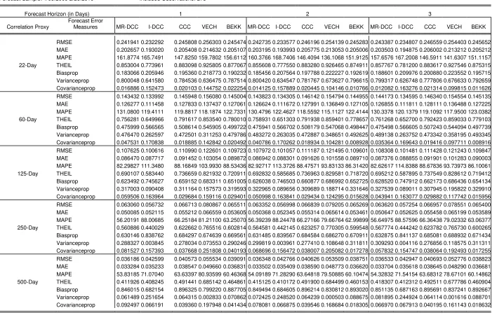
Table 6. Rolling-sample Forecasting Performance of the Mean-Reverting and Integrated DCC, CCC, Diagonal VECH, and Diagonal BEKK Models as Compared to the 22-Day, 60-Day, 125-Day, 250-Day, and 500-Day Realized Correlations for 1-Day to5-Day Forecast Horizons

Forecast Sample: 1/05/2009 2/26/2010 Included Observations: 278

Forecast Horizon (in Days) 1 2 3

Correlation Proxy

Forecast Error

Measures MR-DCC I-DCC CCC VECH BEKK MR-DCC I-DCC CCC VECH BEKK MR-DCC I-DCC CCC VECH BEKK

RMSE 0.241941 0.232292 0.245808 0.256303 0.245474 0.242735 0.233577 0.246196 0.254139 0.245283 0.243387 0.234807 0.246559 0.254403 0.245652

MAE 0.202657 0.193020 0.205408 0.214632 0.205107 0.203195 0.193993 0.205775 0.213053 0.205006 0.203503 0.194875 0.206002 0.213212 0.205212

MAPE 161.8774 165.7491 147.8250 159.7802 156.6112 160.3766 168.7406 146.4094 136.1068 151.9125 157.6576 167.2008 146.5911 141.6307 151.1157

22-Day THEIL 0.853004 0.773961 0.883098 0.925805 0.877067 0.855608 0.777550 0.883280 0.926465 0.874911 0.857767 0.781200 0.883617 0.927546 0.875315

Biasprop 0.183066 0.205946 0.195360 0.218773 0.190232 0.185456 0.207564 0.197788 0.222227 0.192619 0.188601 0.209976 0.200880 0.223552 0.195715

Varianceprop 0.800048 0.641580 0.784536 0.636475 0.787514 0.800420 0.634547 0.781767 0.673627 0.796615 0.799317 0.626748 0.777806 0.676633 0.792659 Covarianceprop 0.016886 0.152473 0.020103 0.144752 0.022254 0.014125 0.157889 0.020445 0.104146 0.010766 0.012082 0.163276 0.021314 0.099815 0.011626

RMSE 0.143432 0.133992 0.145948 0.156080 0.145004 0.143823 0.134305 0.146142 0.154794 0.144955 0.144173 0.134595 0.146340 0.154554 0.145135

MAE 0.126277 0.111458 0.127833 0.137437 0.127061 0.126624 0.111672 0.127991 0.136849 0.127105 0.126855 0.111811 0.128111 0.136488 0.127225

MAPE 131.0800 119.4111 119.8817 118.1874 122.7331 130.4796 122.4627 118.5592 115.1127 122.4144 130.3378 120.1379 119.1092 117.9500 123.0382

60-Day THEIL 0.756281 0.649966 0.791617 0.853540 0.780010 0.758931 0.651303 0.791938 0.859401 0.778657 0.761268 0.652700 0.792423 0.859033 0.779103

Biasprop 0.475999 0.566565 0.508614 0.545905 0.499722 0.475941 0.566702 0.508179 0.547068 0.498447 0.475498 0.566605 0.507243 0.544094 0.497739

RMSE 0.107625 0.100616 0.110990 0.122601 0.109723 0.107972 0.101057 0.111187 0.121495 0.109601 0.108308 0.101481 0.111428 0.121243 0.109847

MAE 0.086470 0.087717 0.091452 0.103054 0.089872 0.086942 0.088301 0.091626 0.101558 0.089710 0.087376 0.088855 0.091901 0.101283 0.090003

MAPE 82.29827 111.3480 88.16849 103.9930 88.53436 82.92717 113.3726 88.47571 93.83133 86.31420 82.62617 114.8388 88.67836 93.73973 86.10061

125-Day THEIL 0.690107 0.583440 0.736659 0.821932 0.720911 0.692832 0.585685 0.736963 0.829581 0.718720 0.695212 0.587895 0.737549 0.828612 0.719412

Biasprop 0.623492 0.745627 0.659152 0.683311 0.651005 0.626038 0.746503 0.660877 0.686992 0.652725 0.628520 0.747912 0.662173 0.686436 0.654134

RMSE 0.063060 0.056732 0.066713 0.080867 0.065511 0.063352 0.056998 0.066839 0.079205 0.065269 0.063620 0.057254 0.066957 0.078551 0.065400

MAE 0.050085 0.052115 0.055212 0.066559 0.053605 0.050368 0.052345 0.055314 0.065614 0.053461 0.050647 0.052625 0.055458 0.065199 0.053589

MAPE 56.20191 88.00685 66.25184 81.21100 63.25070 56.39239 88.24478 66.27166 79.66764 62.99899 56.64975 88.57596 66.36438 79.02332 63.06377

250-Day THEIL 0.560886 0.440029 0.622662 0.765516 0.602814 0.564581 0.442145 0.623257 0.770305 0.599548 0.567774 0.444242 0.623782 0.765730 0.600265

Biasprop 0.630146 0.838762 0.684297 0.674639 0.669561 0.631485 0.839567 0.684584 0.686270 0.670911 0.632875 0.841137 0.685081 0.688932 0.671434

RMSE 0.036186 0.042599 0.040573 0.055534 0.039091 0.036348 0.042766 0.040626 0.053509 0.038751 0.036533 0.042947 0.040693 0.052776 0.038823

MAE 0.033284 0.035233 0.038547 0.049660 0.036831 0.033502 0.035409 0.038590 0.048773 0.036620 0.033704 0.035618 0.038645 0.048290 0.036681

MAPE 53.83185 71.07040 63.63397 80.93599 60.46368 54.09189 71.28290 63.64818 79.50885 60.10474 54.32832 71.54154 63.68312 78.67101 60.14862

500-Day THEIL 0.411926 0.408245 0.491441 0.685142 0.464861 0.415125 0.410172 0.491900 0.684499 0.460153 0.418307 0.412312 0.492511 0.677786 0.460904

Biasprop 0.846015 0.682154 0.896325 0.799220 0.887705 0.849494 0.684605 0.896214 0.830812 0.893020 0.851135 0.687163 0.895691 0.837241 0.892667

(32)

30

Date: 04/02/11 Time: 09:37 Method: Rolling Sample

Forecast Sample: 1/05/2009 2/26/2010 Included Observations: 278

Forecast Horizon (in Days) 4 5

Correlation Proxy Forecast Error Measures MR-DCC I-DCC CCC VECH BEKK MR-DCC I-DCC CCC VECH BEKK

RMSE 0.243950 0.236036 0.246711 0.254366 0.245986 0.244263 0.237160 0.246743 0.253975 0.246089

MAE 0.203839 0.195815 0.205911 0.213144 0.205420 0.203924 0.196594 0.205901 0.212601 0.205364

MAPE 155.2765 163.6263 145.1657 138.3737 150.9919 157.2370 168.1606 146.8039 140.7099 152.4457

22-Day THEIL 0.859475 0.784946 0.883225 0.926630 0.875557 0.860803 0.788964 0.883043 0.924781 0.875607

Biasprop 0.191871 0.212484 0.204387 0.225988 0.198872 0.196556 0.216392 0.209202 0.230269 0.203493

Varianceprop 0.797959 0.619311 0.775276 0.678409 0.788890 0.794592 0.610049 0.770583 0.678519 0.783667

Covarianceprop 0.010170 0.168204 0.020337 0.095603 0.012238 0.008852 0.173559 0.020216 0.091212 0.012840

RMSE 0.144437 0.134762 0.146367 0.154182 0.145268 0.144737 0.135148 0.146529 0.154007 0.145454

MAE 0.127072 0.111911 0.128189 0.136264 0.127301 0.127316 0.112059 0.128322 0.135936 0.127428

MAPE 131.7613 124.4044 119.7189 113.3160 123.3792 131.5127 124.6426 119.3554 111.2964 123.2532

60-Day THEIL 0.763147 0.653766 0.792213 0.856877 0.779432 0.764867 0.655846 0.792507 0.855103 0.779833

Biasprop 0.475024 0.567215 0.507076 0.542979 0.496783 0.474875 0.567039 0.506700 0.541427 0.496184

Varianceprop 0.494504 0.265236 0.475032 0.365098 0.494328 0.498758 0.266109 0.475858 0.370067 0.494958

Covarianceprop 0.030471 0.167549 0.017891 0.091923 0.008889 0.026367 0.166853 0.017442 0.088506 0.008857

RMSE 0.108616 0.101876 0.111610 0.121130 0.110076 0.108913 0.102339 0.111825 0.121031 0.110300

MAE 0.087783 0.089362 0.092033 0.101175 0.090288 0.088228 0.089931 0.092345 0.101093 0.090604

MAPE 82.55399 115.4881 87.72646 94.48875 86.01520 82.39083 116.5598 87.13774 93.16015 86.05260

125-Day THEIL 0.697250 0.590086 0.737818 0.827119 0.719972 0.699014 0.592773 0.738260 0.825132 0.720459

Biasprop 0.631071 0.750056 0.664233 0.686301 0.655553 0.634104 0.752187 0.666479 0.686887 0.657617

Varianceprop 0.331137 0.088676 0.306729 0.199440 0.328276 0.333419 0.088174 0.304937 0.201717 0.326267

Covarianceprop 0.037791 0.161267 0.029038 0.114259 0.016171 0.032477 0.159640 0.028584 0.111395 0.016117

RMSE 0.063916 0.057589 0.067071 0.078264 0.065525 0.064218 0.058018 0.067229 0.077971 0.065670

MAE 0.050905 0.052859 0.055548 0.064933 0.053710 0.051194 0.053194 0.055726 0.064743 0.053881

MAPE 56.82882 88.74503 66.39026 78.41270 63.11558 57.06699 88.93599 66.51929 78.04170 63.24106

250-Day THEIL 0.571014 0.447117 0.624347 0.762782 0.600894 0.574035 0.450776 0.625193 0.758892 0.601599

Biasprop 0.633445 0.841089 0.685909 0.688348 0.671890 0.634732 0.840552 0.687083 0.689489 0.673186

Varianceprop 0.316558 0.004344 0.276555 0.123945 0.310756 0.321462 0.004541 0.275264 0.127854 0.309335

Covarianceprop 0.049997 0.154566 0.037536 0.187706 0.017354 0.043806 0.154907 0.037653 0.182657 0.017479

RMSE 0.036726 0.043134 0.040732 0.052362 0.038881 0.036926 0.043350 0.040811 0.051963 0.038955

MAE 0.033891 0.035847 0.038651 0.047954 0.036731 0.034081 0.036110 0.038711 0.047662 0.036800

MAPE 54.54448 71.83720 63.63067 78.02135 60.18444 54.76577 72.12781 63.66107 77.54149 60.23727

500-Day THEIL 0.421440 0.414697 0.492906 0.672909 0.461467 0.424427 0.417490 0.493705 0.667290 0.462159

Biasprop 0.851561 0.690278 0.896602 0.838727 0.892433 0.851879 0.693864 0.896672 0.841299 0.892407

Varianceprop 0.089972 0.240417 0.064276 0.002482 0.088732 0.096607 0.235193 0.064179 0.003215 0.088539

(33)

[image:33.595.76.496.284.596.2]

31

Table 7. Diebold-Mariano Tests of Predictive Accuracy using the Squared Error Loss of the Integrated Dynamic Conditional Correlation Models versus the Mean-Reverting Dynamic Conditional Correlation Model, Constant Conditional Correlation Model, Diagonal VECH Model, and Diagonal BEKK Model using the 22-Day, 60-Day, 125-Day, 250-Day, ad 500-Day

Realized Correlations as Proxy for the True Correlation

Null Hypothesis: Integrated DCC has equal predictive accuracy as the other model

Alternative Hypothesis: Integrated DCC has greater predictive accuracy than the other model Date: 04/06/11 Time: 07:49

Forecast Sample: 1/05/2009 2/26/2010 Method: Rolling Sample

Correlation Proxy Forecast Horizon MR-DCC CCC VECH BEKK

1-Day -1.68* -2.35*** -3.30*** -2.32*** 2-Day -1.58 -2.19** -2.83*** -2.05** 22-Day 3-Day -1.46 -2.04** -2.72*** -1.90* 4-Day -1.34 -1.85* -2.56*** -1.74* 5-Day -1.20 -1.66* -2.35*** -1.56 1-Day -2.25** -2.90*** -4.12*** -2.67*** 2-Day -2.28** -2.91*** -3.95*** -2.63*** 60-Day 3-Day -2.30** -2.92*** -3.89*** -2.63*** 4-Day -2.33*** -2.89*** -3.87*** -2.64*** 5-Day -2.29** -2.83*** -3.74*** -2.59*** 1-Day -1.44 -2.06** -3.17*** -1.86* 2-Day -1.41 -1.99** -2.89*** -1.73* 125-Day 3-Day -1.38 -1.94* -2.80*** -1.68* 4-Day -1.35 -1.89* -2.73*** -1.64 5-Day -1.30 -1.83* -2.66*** -1.58 1-Day -0.83 -1.25 -2.29** -1.11 2-Day -0.83 -1.23 -2.12** -1.06 250-Day 3-Day -0.83 -1.22 -2.06** -1.05 4-Day -0.83 -1.20 -2.03** -1.03 5-Day -0.82 -1.18 -1.99** -1.00 1-Day 0.77 0.26 -1.43 0.44 2-Day 0.77 0.27 -1.17 0.50 500-Day 3-Day 0.77 0.29 -1.08 0.52 4-Day 0.77 0.30 -1.02 0.53 5-Day 0.78 0.32 -0.96 0.55

(34)

[image:34.595.74.522.194.518.2]

32

Figure 15. Time Plots of the Forecasted Dynamic Out-of-Sample Correlations between the Log Returns of the Peso-Dollar Exchange Rate and the Philippine Stock Exchange Index from January, 2009 to February, 2010 using the Mean-Reverting and Integrated Dynamic Conditional

Correlation Models, Constant Conditional Correlation Model, Diagonal VECH Model, and Diagonal BEKK Model

-.026 -.024 -.022 -.020 -.018 -.016 -.014 .0220 .0225 .0230 .0235 .0240 .0245 .0250

M1 M2 M3 M4 M5 M6 M7 M8 M9 M10 M11 M12 M1 M2

2009 2010

Forecasted Correlations using Mean-Reverting DCC Forecasted Correlations using Integrated DCC Forecasted Correlation using CCC

Forecasted Correlations using Diagonal VECH Forecasted Correlations using Diagonal BEKK

(35)

[image:35.595.76.549.207.622.2]

33

Table 8. Dynamic Forecasting Performance of the Mean-Reverting DCC, Integrated DCC, CCC, Diagonal VECH, and Diagonal BEKK Models as Compared to the 22-Day, 60-Day, 125-Day,

250-Day, and 500-Day Realized Correlations Date: 04/01/11 Time: 11:25

Forecast Sample: 1/05/2009 2/26/2010 Method: Dynamic

Correlation Proxy Forecast Error Measures MR-DCC I-DCC CCC VECH BEKK