Enhancing Estimation for Interest Rate Diffusion Models with Bond Prices

Munich Personal RePEc Archive

Enhancing Estimation for Interest Rate

Diffusion Models with Bond Prices

Zou, Tao and Chen, Song Xi

Peking University, Peking University

January 2014

Online at

https://mpra.ub.uni-muenchen.de/67073/

Enhancing Estimation for Interest Rate

Diffusion Models with Bond Prices

Tao Zou and Song Xi Chen∗

Department of Business Statistics and Econometrics

Guanghua School of Management and Center for Statistical Science

Peking University

Abstract

We consider improving estimating parameters of diffusion processes for interest rates by

incorporating information in bond prices. This is designed to improve the estimation of the

drift parameters, which are known to be subject to large estimation errors. It is shown that

having the bond prices together with the short rates leads to more efficient estimation of all

parameters for the interest rate models. It enhances the estimation efficiency of the maximum

likelihood estimation based on the interest rate dynamics alone. The combined estimation

based on the bond prices and the interest rate dynamics can also provide inference to the

risk premium parameter. Simulation experiments were conducted to confirm the theoretical

properties of the estimators concerned. We analyze the overnight Fed fund rates together

with the U.S. Treasury bond prices.

JEL CLASSIFICATION: C50, C58.

Key words: Interest Rate Models; Affine Term Structure; Bond Prices; Market Price of

Risk; Combined Estimation; Parameter Estimation.

1

Introduction

Interest rate models especially those for the short rates, as basic financial instruments and

mea-sures for the risk-free assets, have attracted much attention in financial and econometric studies.

Modeling the term structure of the interest rates is a focal point of these studies. Diffusion

pro-cesses constitute a popular class of models for the interest rate dynamics. The Vasicek and the

CIR diffusion models, introduced in Vasicek (1977) and Cox, Ingersoll and Ross (1985), and the

much broader affine term structure models (Duffie and Kan, 1996; Dai and Singleton, 2000; Duffee,

2002) are the basic interest rate models for pricing the zero-coupon or coupon bearing bonds and

interest rate derivatives.

It is known that the drift parameters of the diffusion processes are more difficult to estimate

than the diffusion parameters, as shown in Phillips and Yu (2005) and Tang and Chen (2009).

This is because that the drift part contains far less information since it is of a smaller order as

compared to the diffusion part. Despite this understanding, the pricings of bonds and interest rate

derivatives require better estimation of the drift parameters as well as parameters which define

the risk premium process. The latter cannot be identified under the physical measure.

In this paper, we consider estimating parameters of interest rate diffusion processes by utilizing

the interest rate data along with the bond prices. We first analyze the least squares estimation

based on the converted zero-coupon bond prices only under the affine term structure models

without using the interest rate data. Although it is known (Brown and Dybvig, 1986) that the

least squares estimation cannot identify all the parameters due to a collinearity, we provide explicit

descriptions on which linear combination of the original parameters can be identified, and propose

a method that selects the largest number of equations from the redundant least squares estimating

equations.

To utilize the bond prices, we propose a framework that combines the short rate data and the

model with the bond prices to improve the parameter estimation of the short rate parameters. The

combined estimation is designed to achieve two goals. One is to improve the estimation efficiency

goal is to identify all the parameters including those of the risk premium. Since the combined

estimation has the extra bond prices and their model information, it enhances the estimation

based on the interest rates only. This is attractive as it improves the MLE of the drift parameters

which are known to have larger estimation errors (Tang and Chen, 2009). We analyze the Federal

fund overnight rates together with the treasury bond prices from 1972 to 2012 to demonstrate our

proposal.

The paper is structured as follows. Section 2 introduces the interest rate models and the

associated bond pricing. Section 3 analyzes the issues for the least squares estimation based on

the bond prices. Section 4 proposes the combined estimation approach that utilizes both the

interest rates and bond prices, whose theoretical properties are given in Section 5. Numerical

results from simulation experiments which compared different estimators are reported in Section

6. Section 7 analyzes the overnight rates of the Federal Reserve and the U.S. Treasury bond

prices. A conclusion is made in Section 8. Assumptions and theoretical proofs are relegated to

the Appendix.

2

Interest Rate Models and Bond Prices

Let r(t) be the short rate at time t. Under the physical measure Q0, the short rate follows a

diffusion process

dr(t) = µ0{t, r(t);β}dt+σ{t, r(t);β}dW0(t), (2.1)

whereµ0(·) andσ(·) are respectively the drift and diffusion functions, βis aq×1 vector containing

the model parameters and W0(t) is the standard Brownian motion under Q0. The maximum

likelihood estimation (MLE) has been a popular method for parameter estimation. Suppose that

the short rates are stationary and we observe the short rates at equally spaced time interval δ:

r(0), r(δ)_{· · ·} , r(nδ). To simplify notations we write r(tδ) as rt by hiding δ.

physical measure Q0. The log-likelihood function of the parameterβ is ∑nt=1ℓt(β), where

ℓt(β) = logft(rt|rt−1, δ;β). (2.2)

The MLE ˜βn solves the score equation ∑n_t=1∂ℓ_∂βt(β) = 0. If the diffusion process (2.1) is time homogeneous and stationary, the consistency and the asymptotic normality of the MLE have

been well understood; see for instance Chang and Chen (2011). If the diffusion process (2.1) is

time inhomogeneous, the likelihood score is still a sum of martingale differences, but the differences

are no longer identically distributed. The asymptotic normality of the MLE can still be established

based on the martingale central limit theorems (Hall and Heyde, 1980).

Popular models for the short rates include the Vasicek model (Vasicek, 1977) which is dr(t) =

κ_{α₋r(t)_}dt +σdW0(t), namely an Ornstein-Uhlenbeck process under Q0. Cox et al. (1985)

proposed using Feller (1951)’s square root diffusion processdr(t) = κ_{α₋r(t)_}dt+σ√

r(t)dW0(t)

to model the short rates with positive parametersκ, αandσsuch that 2κα/σ2 _{>1. The analytical}

forms of the transition densities for these two processes are known to be the densities of a normal

and a non-central chi-squared ones, respectively, which facilitate the MLEs. For interest rate

diffusion models whose transition densities are unknown, which is often the case, A¨ıt-Sahalia

(1999, 2002)’s approximate MLE can be employed.

Despite the MLE or the approximate MLE being consistent and asymptotically normal, the

estimation for the drift parameters encounters a slower rate of convergence (√nδ) and a large order of bias ((nδ)−1_{) as revealed in Tang and Chen (2009). In contrast, the convergence rate of}

the estimation for the diffusion parameter is √n and the bias is of order n−1_{, which are much}

smaller than those of the drift parameter.

A new initiative is needed to improve the parameter estimation as the pricing of bonds and

interest rate derivatives requires more accurate estimation of the drift parameters as well as

parameters which define the risk premium process. The latter cannot be identified in the short

rate process under the physical measure. Our proposal is to bring in bond prices under an interest

rate diffusion model to produce a more efficient combined estimation of the parameters.

zero-coupon bond at time t that matures at a future time s > t. In order to discuss the bond

pricing theory, the short rate given in (2.1) is considered under the risk-neutral measure Q1:

dr(t) = µ1{t, r(t);θ}dt+σ{t, r(t);θ}dW1(t) (2.3)

= [µ0{t, r(t);β}+σ{t, r(t);β}Λ{t, r(t);λ}]dt+σ{t, r(t);β}dW1(t),

where W1(t) is the standard Brownian motion under Q1, θ = (β′, λ′)′ is a (q +d)×1 vector

of parameters with a new d-dimensional parameter λ that defines the market price of risk, and

Λ(t) := Λ_{t, r(t);λ_} is the market price of risk process relying on the parameter λ. The two measures Q0 and Q1 are connected through the Girsanov change of measure.

If r(t) follows an one-factor affine term structure model, namely

µ1{t, r(t);θ}=K0(t;θ) +K1(t;θ)r(t) and σ2{t, r(t);θ}=H0(t;θ) +H1(t;θ)r(t), (2.4)

for some deterministic functions K0(·), K1(·), H0(·) and H1(·) of t and θ, respectively, then based

on the no-arbitrage pricing theory, the bond priceP(t, s) is shown to satisfy (Duffie, 2001)

−logP(t, s) =A(t, s;θ) +B(t, s;θ)r(t), (2.5) and the pricing functionsA(t, s;θ) andB(t, s;θ) are determined by the Riccati differential equation

∂B(t, s;θ)

∂t =

1

2H1(t;θ)B

2_{(t, s;θ)−K}

1(t;θ)B(t, s;θ)−1; B(s, s;θ) = 0 (2.6)

and an integral equation

A(t, s;θ) = ∫ s

t {

K0(u, θ)B(u, s;θ)−

1

2H0(u;θ)B

2_{(u, s;θ)}

}

du. (2.7)

To illustrate the key ingredients in the affine term structure, we consider two specific affine

mod-els: the Vasicek and CIR models. Under the risk-neutral measureQ1, the Vasicek model follows

(Brigo and Mercurio, 2006)dr(t) = [κ_{α₋r(t)_}+σλr(t)]dt+σdW1(t),whereλis the univariate

market price of risk parameter, while the CIR model admits dr(t) = [κ_{α₋r(t)_}+σλr(t)]dt+ σ√r(t)dW1(t). Both the Vasicek and CIR models have explicit expressions of B(t, s;θ) and

structure models which do not have explicit B(_·) andA(_·), numerical solutions to the differential equation (2.6) and the integral equation (2.7) can be attained, for example using the Runge-Kutta

discretization method in Hairer, Nøersett and Wanner (2006).

3

Generalized Least Squares Estimation

It is worth noting that the observed bonds in a fixed income market are most likely coupon-bearing.

There are methods to convert coupon-bearing bond prices to the zero-coupon bond prices, such

as the bootstrap method of Hull (2009), the parametric method of Nelson and Siegel (1987) and

Svensson (1994), and the spline method of McCulloch (1975, 1993) and Vasicek and Fong (1982).

Suppose that by one of the above conversion methods, at a date t we have M zero-coupon

bonds with time to maturitiesτ1, τ2,· · · , τM which do not depend ont. Letpit =−logP(tδ, tδ+τi) be the transformed zero-coupon bond price at time t with maturity τi. As consequences of the

conversion procedures to get the zero-coupon bond prices and the uncertainty with the models and

the randomness in the observed prices, measurement errors are inevitably present in the observed

bond prices. Hence, pit can deviate from (2.5) such that

pit =Ait(θ0) +Bit(θ0)rt+u0it, fori= 1,· · · , M; t = 1,· · · , n; (3.1) where u0it denotes the pricing error, Ait(θ) := A(tδ, tδ+τi;θ0), Bit(θ) := B(tδ, tδ+τi;θ0) and θ0

is the true parameter. In the above, i is a shorter version of τi. Model (3.1) has been considered

in literatures (Pearson and Sun, 1994; Duffee, 2002; Cheridito, Filipovi´c and Kimmel, 2007;

A¨ıt-Sahalia and Kimmel, 2010) and the number of bonds M used is rather smaller than the sample

size n. Hence we assume M is fixed.

Let pt = (p1t,· · · , pM t)′, At(θ) = (A1t(θ),· · · , AM t(θ))′, Bt(θ) = (B1t(θ),· · · , BM t(θ))′ and u0t= (u01t,· · · , u0M t)′. Then, (3.1) can be written as

pt=At(θ0) +Bt(θ0)rt+u0t. (3.2)

the filtration _{Gt}, where Gt is the σ-algebra generated by {(rl+1, u′0l)′}l≤t. The generalized least squares (GLS) estimator of θ can be attained by minimizing

n ∑

t=1

{pt−At(θ)−Bt(θ)rt}′W{pt−At(θ)−Bt(θ)rt}, (3.3) for an M _×M positive definite weighting matrix W. Then the GLS estimator solves

n ∑

t=1

gt(θ;W) = 0, (3.4)

wheregt(θ;W) = {

∂At(θ)

∂θ′ +

∂Bt(θ)

∂θ′ rt

}′

W ut(θ) for ut(θ) =pt−At(θ)−Bt(θ)rt.

However, (3.4) cannot identify all of the parameters in θ. This is because the dynamics

under the risk neutral measure can be specified with a parameter transformation ϑ=ϑ(θ) whose

dimension is less than that of θ. This implies that Model (2.3) under the risk neutral measure Q1

can be written as

dr(t) = ˜µ1{t, r(t);ϑ}+ ˜σ{t, r(t);ϑ}dW1(t). (3.5)

For instance, the Vasicek and CIR models in Section 2 can be expressed with three parameters

under the risk neutral measure via a new parameterization: b =κ₋σλ, a= κα

κ−σλ and σ, rather than the four parameters in θ = (κ, α, σ, λ)′_{. As a result, the pricing functions A}

t(θ) and Bt(θ) may be written via the smaller set ϑ so that Bt(θ) = ˜Bt(ϑ) and At(θ) = ˜At(ϑ) in (2.6) and

(2.7). This means that (3.4) has redundant equations. The redundancy has been noticed in the

literatures, for instance in Brown and Dybvig (1986). However, what has not been considered in

the literatures is the selection of the non-redundant equations in (3.4) and how to use them to

improve the estimation of parameters. We will investigate these issues in the following section.

4

Combined Estimation

In this section, we propose an estimation method that combines the MLE approach based on the

interest rate dynamics, with the use of the non-redundant equations in the GLS estimation based

the estimation efficiency of the MLE revealed in Section 2, and enable the estimation of the risk

premium parameter, as well as repair the identification issue of the GLS estimation.

If the short rate under (2.1) and (2.3) is time homogenous, then one can show that the transition

density ft(·) as well as At(·) and Bt(·) are time homogeneous too such that ft(rt|rt−1, δ;β) =

f(rt|rt−1, δ;β), At(θ) = A(θ) and Bt(θ) =B(θ). We focus on the time homogeneous case in the following. Extension to the time inhomogeneous case can be made with more involved notations

and technical details, which is discussed in Section 8.

To start with, we select a set of non-redundant equations in (3.4), denoted by_E′_g

t(θ;W) where

E is a matrix consisting ofq† _{columns of the identity matrix I}

q+d and q†< q+d is the maximum number of non-redundant equations. As ∑n

t=1E′gt(θ;W) = 0 can not identify θ, we combine it with the likelihood score to form a combined generalized method of moment (GMM) equations

ht(θ;E, W) = 



∂ℓt(β)

∂β

E′_g

t(θ;W) 

, (4.1)

which hasq+q† _{moment conditions for q+d unknown parameters. It is noted that, atθ}

0,

E{ht(θ0;E, W)}= 0. (4.2)

LetV0 =E(u0tu′0t|Gt−1) =: (vjk)M×M be the conditional covariance matrix of the measurement errors, which is assumed to be of full rank. For a given W, the optimal GMM estimation utilizes

a weighting matrix which is the inverse of the long-run covariance

Σh(θ0;E, W) =: lim

n→∞nVar

{ 1 n

n ∑

t=1

ht(θ0;E, W)

}

. (4.3)

This implies thatq† _{and E should be chosen properly to make Σ}

h(θ0;E, W) invertible.

Let _I0(δ) be the Fisher information matrix associated with the likelihood score for β,

ψ(θ0) :=



 ∂A(θ0)

∂θ′ +

∂B(θ0)

∂θ′ E(rt)

∂B(θ0)

∂θ′

√

Var(rt) 



Proposition 4.1. Under Assumptions 1 - 5 given in Appendix, and for any δ _∈ (0,∆1] where

∆1 >0 is a finite constant, Σh(θ0;E, W) = diag{I0(δ),Ξ0(E, W)}.

The proposition implies that Σh(θ0;E, W) is invertible if and only if both I0(δ) and Ξ0(E, W)

are invertible. Since _I0(δ), V0 and W are nonsingular, we only require ψ(θ0)E to be of full rank

for the largest possible q†_.

We select _E from the following set

{E :ψ(θ0)E form a largest collection of linearly independent columns of ψ(θ0)} (4.4)

where q† _{:= rank{ψ(θ}

0)} = rank{ψ(θ0)E}. As (4.4) has more than one element, different Es in

(4.4) select different non-redundant equations in the score gt(θ;W). Theorem 5.2 will show that

the combined estimators attain the same asymptotic efficiency despite using different _Es in (4.4). For both the Vasicek and CIR models, it is illustrated in the supplementary material that if

there is only one bond available at each t, namely M = 1, _E can be any two columns of I4 with

q† _{= 2; and if there are at least two bonds, namely M ≥ 2, E can consist of three columns of I}

4

which must has the third column of I4, with q† = 3. We note that the third column corresponds

to the diffusion parameter σ for θ = (κ, α, σ, λ)′_{. Since q}† _{is at least 2 which is larger than d= 1}

for the Vasicek and CIR models, the proposed combined estimation is able to identify all the

parameters including the market price of risk parameter.

In order to carry out the GMM estimation, an initial estimation of θ is needed to estimate the

weighting matrix Σ−1

h (θ0;E, W), which is

¯

θn(E, W) = arg min θ∈Θ

{ 1 n

n ∑

t=1

ht(θ;E, W) }′{

1 n

n ∑

t=1

ht(θ;E, W) }

.

Let ˆ_In(β) = 1_n∑nt=1

∂ℓt(β)

∂β ∂ℓt(β)

∂β′ and ˆΞn(θ;E, W) = _n1 ∑nt=1E′gt(θ;W)gt(θ;W)′E. Write ¯θn(E, W) = (¯

βn(E, W)′,λ¯n(E, W)′ )′

. Define the estimated weighting matrix

ˆ

W_{n(E, W) := diag}{_Iˆ−1

n (¯

βn(E, W) )

,Ξˆ−_n1(¯

θn(E, W);E, W )}

The proposed combined (GMM) estimator for θ, consisting of both the interest rate parameter β

and the risk premium parameter λ, is

ˆ

θn(E, W) = arg min θ∈Θ

{ 1 n n ∑ t=1

ht(θ;E, W) }′

ˆ

W_{n(E, W)}

{ 1 n n ∑ t=1

ht(θ;E, W) }

. (4.5)

5

Theoretical Results

The theoretical properties of the combined estimator for θ are presented in this section. We first

need to define a few matrices to convey the asymptotic normality of the combined estimator. Let

G0(E, W) :=E

{ ∂_E′_g

t(θ0;W)

∂θ′

}

=_−E′ψ(θ0)′(I2 ⊗W)ψ(θ0), (5.1)

H0(δ;E, W) :=E

{

∂ht(θ0;E, W)

∂θ′

} =





(_−I0(δ),0q×d) G0(E, W)



 and

Q0(δ;E, W) := H0(δ;E, W)′diag

{

I0−1(δ),Ξ−01(E, W)

}

H0(δ;E, W)

= 



I0(δ) 0q×d 0d×q 0d×d



+G0(E, W)′Ξ0−1(E, W)G0(E, W)

=: 



Q11,0(δ) Q12,0 Q21,0 Q22,0



, say. (5.2)

Furthermore, let

Ω(δ;_E, W) :=_Q11,0(δ)− Q12,0Q−221,0Q21,0, (5.3)

where _Q22,0 is invertible under Assumption 6. It can be checked that Q0(δ;E, W) is invertible

based on Lemma A.4 in the Appendix for any δ_∈(0,∆1] and

Q−01(δ;E, W) =





Ω−1_{(δ;E, W) −Ω}−1_{(δ;E, W)Q}

12,0Q−221,0

−Q22−1,0Q21,0Ω−1(δ;E, W) Q−221,0+Q22−1,0Q21,0Ω−1(δ;E, W)Q12,0Q−221,0



. (5.4)

Theorem 5.1. Under Assumptions 1 - 6 given in Appendix, for any δ _∈(0,∆1] as n → ∞, √

n_Q10/2(δ;E, W)

( ˆ

θn(E, W)−θ0

) _d

Theorem 5.1 implies that the asymptotic variance (Avar) of ˆθn(E, W) is n−1Q−01(δ;E, W). It

is known that the asymptotic variance of the MLE ˜βn based on the short rates only isn−1I0−1(δ).

Write ˆθn(E, W) = (

ˆ

βn(E, W)′,ˆλn(E, W)′ )′

where ˆβn(E, W) is the new estimator of β by the proposed combined estimation and ˆλn(E, W) is the estimator of the risk premium parameter. From (5.4),

Avar(βˆn(E, W) )

=n−1Ω−1(δ;_E, W) and Avar(λˆn(E, W)

)

=n−1_Q−₂₂1_,0+n−1_Q−₂₂1_,0Q21,0Ω−1(δ;E, W)Q12,0Q−221,0 =O

(

n−1δ−1) .

The following corollary shows that the combined inference for β is at least as efficient as the

MLE ˜βn based on the interest rates. The bond information indeed enhances the estimation.

Corollary 5.1. Under Assumptions 1 - 6 given in Appendix, for any positive definite W, and _E satisfying (4.4), then Avar(βˆn(E, W)

)

≤Avar(β˜n )

for any δ _∈(0,∆1].

Recall that different _Es in set (4.4) select different GLS moment restrictions in gt(θ;W). The following theorem shows that different _Es lead to the same asymptotic efficiency as long as they satisfy (4.4).

Theorem 5.2. Under Assumptions 1 - 6 given in Appendix, for any two _E1 ̸=E2 satisfying (4.4),

Avar(θˆn(E1, W) )

=Avar(θˆn(E2, W) )

.

Since usually the number of the moment conditions q +q† _{> q +d (e.g., in both Vasicek}

and CIR models introduced in Section 2), we can perform the over-identification test (theJ-test,

Hansen, 1982) to check on the appropriateness of

H0 :E{ht(θ0;E, W)}= 0 versus H1 :E{ht(θ0;E, W)} ̸= 0. (5.5)

The J-statistic is

Jn=n {

1 n

n ∑

t=1

ht (

ˆ

θn(E, W);E, W )

}′ ˆ

W_{n(E, W)}

{ 1 n

n ∑

t=1

ht (

ˆ

θn(E, W);E, W )

}

,

which can be shown to converge to χ2_q†_−d in distribution under H0 based on Theorem 5.1.

J-test (5.5) is rejected, then the moment condition (4.2), which is decided by different affine term

structure models and the exogeneity of the measurement errors, is not appropriately specified.

Hence the J-test (5.5) provides a model selection criterion to decide which of the affine models

(e.g., Vasicek or CIR) is preferred for the data.

Now let us consider the role of W.

Corollary 5.2. Under Assumptions 1 - 6 given in Appendix, for any δ _∈ (0,∆1], as n → ∞,

Avar(θˆn(E, V0−1)

)

≤Avar(θˆn(E, W) )

for any positive definite W.

Corollary 5.2 implies that choosing W = V−1

0 leads to the efficient estimator of θ for each given E. This is consistent with the theory of the GLS method and implies that gt(θ;V0−1) should be

used if we have the knowledge ofV0.

It is noted that the efficiency lower bound is n−1 _{times the inverse of}

Q0(δ;E, V0−1) =





I0(δ) 0q×d 0d×q 0d×d



+ψ(θ0)′

(

I2⊗V0−1

)

ψ(θ0). (5.6)

Hence, the accuracy of the combined estimation is adversely influenced byV0, the variance of the

measurement errors, although it is still more accurate than the MLEs for β.

We now consider the impact of M, the number of bonds used in the inference.

Corollary 5.3. Under Assumptions 1 - 6 given in Appendix, when the number of bonds M

in-creases, Avar(θˆn(E, V0−1)

)

does not increase for any V0.

Corollary 5.3 means that ifW =V−1

0 , the more bonds we include in the estimating procedure, the

more efficient the estimators are. However, this may not be true ifW _̸=V−1

0 , which is confirmed

in our numerical study reported later, namely the bond prices can improve the efficiency only if

we consider the measurement error structure of the new information.

As V0 is unknown in practice, we consider the following “sample covariance” estimator

ˆ Vn(E) =

1 n

n ∑

t=1

ut (

ˆ

θn(E, IM) )

ut (

ˆ

θn(E, IM) )

It can be shown that under Assumptions 1 - 6 given in Appendix, for any δ_∈(0,∆1]

ˆ Vn(E)

p

−→V0 as n→ ∞. (5.8)

With ˆVn(E), we get ˆθn(E,Vˆn−1(E)) which we call the feasible combined estimator of θ. It can be shown that ˆθn(E,Vˆn−1(E)) attains the same asymptotic efficiency as ˆθn(E, V0−1).

We can also estimate the asymptotic variance n−1_Q−1

0 (δ;E, W) upon given E and W. From

(5.1),

G0(E, W)

= −E′

[ ∂A(θ0)′

∂θ W

∂A(θ0)

∂θ′ +E(rt)

{ ∂A(θ0)′

∂θ W

∂B(θ0)

∂θ′ +

∂B(θ0)′

∂θ W

∂A(θ0)

∂θ′

}

+E(r2 t)

∂B(θ0)′

∂θ W

∂B(θ0)

∂θ′

]

=: G{θ0,E(rt),E(r 2 t);E, W

}

, say.

Let

ˆ

Gn(E, W) = G

{ ˆ

θn(E, W),

1

n n

∑

t=1

rt,

1

n n

∑

t=1

r2_t;_E, W

}

and

ˆ

Qn(_E, W) =

   ˆ In ( ˆ

βn(E, W)

) 0q×d

0d×q 0d×d





+ ˆGn(E, W)

′_Ξˆ−1

n

( ˆ

θ_n(_E, W);_E, W)Gˆ_n(_E, W). (5.9)

It can be shown by a routine derivation that ˆ_Qn(E, W) is a consistent estimator of Q0(δ;E, W),

which can be used in forming confidence intervals and testing hypothesis for each parameter.

Let us summarize the key steps in carrying out the proposed combined estimation. After

having the interest rate data _{rt}nt=0 and the bond prices {pt}nt=1, a model from the affine term

structure models (e.g., Vasicek or CIR) is identified, followed by finding the matrix _{E ∈}R(q+d)×q† from (4.4) to select the maximum non-redundant estimating equations in (3.4). We then carry

out the GMM estimation ˆθn(E, IM) in (4.5) with the initial weight matrix W = IM. Finally, we obtain the efficient GMM estimator ˆθn(E,Vˆn−1(E)) in (4.5) and its estimated standard error via (5.9) by letting W = ˆV−1

6

Simulation Studies

We report results of simulation experiments which were designed to confirm the theoretical findings

in the previous section. We specifically want to check on the efficiency gain of the combined

estimators by comparing with the MLE or the approximate MLE in the context of the Vasicek

and CIR models. The full MLE was employed for the Vasicek model, while the approximate MLE

based on a two-term expansion (A¨ıt-Sahalia, 1999, 2002) was employed for the CIR. The latter

was to evaluate the approximate MLE in our context, though the full MLE for the CIR can be

conducted. The parameters used for both models were (κ, α, σ, λ) = (0.892,0.09,√0.033,0.1), with the monthly sampling interval δ = 1/12. The sample size n was 300, 500, 1000 and 2000,

respectively. All the simulation results were base on 2000 simulations.

The simulated short rates were generated from both processes via their known transition

distributions with the initial value from their known stationary distributions, respectively. In the

simulation of the bond prices, we considered two designs for the maturity. One had fifteen bonds

(M = 15) with the time to maturity ranging from 6 months to 7.5 years; and the other had five

bonds (M = 5) which have the time to maturity ranging from 6 months to 2.5 years. Both settings

had six months between two adjacent maturities. The bond prices were generated according

to (3.2) with the measurement errors _{u0t} iid

∼ N(0, V0). Following the analysis of Cheridito

et al. (2007) and A¨ıt-Sahalia and Kimmel (2010), we designed V0 = diag{v12, v22,· · · , vM2 }, and let vi = 0.001×3τi for i = 1,· · · , M. The specification above implies that the measurement errors were independent ofrtand was homogeneous with respect to the time, and the standard deviations

of the errors increased exponentially with respect toτi. As a consequence of the diagonal form of

V0, we only need to estimate the diagonal elements instead of the estimation in (5.7), namely

ˆ

Vn(E) = diag {

1 n

n ∑

t=1

ut (

ˆ

θn(E, IM) )

ut (

ˆ

θn(E, IM) )

}

.

On the other hand, since we had more than two bonds, we chose _E1 = (e2, e3, e4) and E2 =

(e1, e2, e3) to select the moments for the proposed combined estimators, where the four dimension

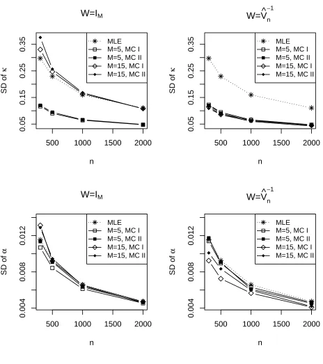
We evaluated the MLEs and the approximate MLEs for β, and the combined estimators for

θ = (β′_{, λ)}′_{. Figures 1 - 3 display the standard deviation and the averaged absolute bias of the}

estimates for the CIR model. The results for the Vasicek model were largely similar and are given

in the supplementary material. We did not report the bias for α and σ since they are of much

smaller order (Tang and Chen, 2009). The most striking feature emerged from these figures are (i)

the feasible combined estimators (withW = ˆV−1

n (E)) offered much improvement in the standard deviations of κ, α and σ, and in the bias ofκ, over those of the MLEs/approximate MLEs. The

amount of improvement offered by the feasible combined estimator varied among the parameters,

with the most improvement registered for κ in both the standard deviation and the bias. This is

very encouraging since the mean reverting parameter is the most difficult to estimate. Another

feature conveyed from these figures is that the combined estimates without using the optimal

weight, namely W = IM, may not be able to produce the best possible performance. However,

when the sample size were increased, the combined estimation with both forms ofW were better

than the MLEs. The estimation error forσ is known (Tang and Chen, 2009) to be much smaller

than the bias of the drift parameters k and α. These were clearly reflected in the vertical scales

of the respective panels for the three parameters.

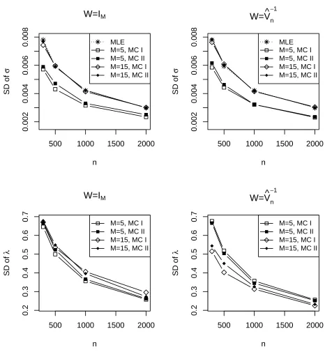
The scale of estimation errors for λ was much larger than those of the other parameters

despite that λ was much smaller than κ and was only slightly larger than α. The reduction in

the estimation errors for λ was quite slow as n was increased. These confirmed the well known

challenge in the estimation of the risk premium parameter. We observed that usingM = 15 bonds

produced smaller standard deviations than those of using M = 5 bonds for the feasible combined

estimator with W = ˆV−1

n (E). This was not necessarily the case for the combined estimator with W =IM. The latter suggested we need to use the feasible estimator to ensure the quality of the

combined estimator when more bond prices are brought into the inference as they may be subject

to more errors along with the increased maturity. We also note that, as the sample size went

7

Case Study

We analyze the US short interest rates in conjunction with the treasury bond prices, and

demon-strate the proposed combined estimation approach. We used the Federal funds overnight rates as

proxies to the short rates. The data series was between January 1972 and December 2012, sampled

at monthly frequency. The source of the overnight rates is the H.15 Federal Reserve Statistical

Release Series. Part of the series (with a different time range) was analyzed in A¨ıt-Sahalia (1999)

who also used the overnight rates as proxies for the short rates. The zero-coupon bond prices

were obtained from the monthly zero-coupon yields over the same time period as the Federal

funds overnight rate series, constructed by G¨urkaynak, Sack and Wright ( 2007) who have been

updating the bond yield data on the Federal Reserve Board Finance and Economics Discussion

Series. There weren = 491 bond prices with the time to maturity ranging from 1 to 15 years. We

grouped the bonds to five categories according to the maturity: 1-3 years, 1-5 years, 1-10 years,

1-15 years and 6-15 years. The combined estimators for each category were conducted to gain

insight on the impact of the maturity on the parameters.

We estimated the parameters of the Vasicek and CIR models introduced in Section 2

respec-tively. The proposed combined estimator with W =IM and W = ˆVn−1(E) were considered. The MLEs for Vasicek and the approximate MLEs for CIR were computed to serve as the

bench-marks of estimation. For the combined estimation, we used _E1 = (e2, e3, e4) (Moment Conditions

I) and _E2 = (e1, e2, e3) (Moment Conditions II). The standard errors of the combined estimates

were obtained by estimating the asymptotic variance via (5.9) in Section 5, and those of the

MLEs/approximate MLEs were obtained by the estimated Fisher information matrices. The

es-timated Fisher information matrix for the approximate MLE under the CIR model was based

on Theorem 4 in Chang and Chen (2011). We also obtained the estimated measurement errors

(estimated residuals) and the covariance of the measurement errors according to (5.7).

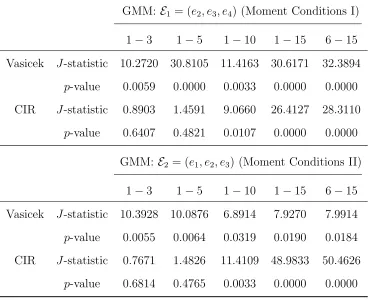
Table 1 reports the p-values of theJ-tests (5.5) for the Vasicek and CIR models with respect

to the five categories of maturity based onW =IM and Moment Conditions I and II. TheJ-tests

found empirical support to the CIR model for shorter maturity of 1-3 years and 1-5 years, as

reflected by the quite large p-values. However, as the maturity range was expanded to more than

10 years, the p-values of the CIR model became quite small, indicating that the model was no

longer reasonable. We recall the work of Chen, Gao and Tang (2008), which conducted

goodness-of-fit tests of the Vasicek and CIR models for the same series of short rates with a different

time range (without considering the bond prices). They found that while the Vasicek model was

severely mis-specified, there was quite some empirical support to the CIR model. This finding was

also consistent with the market segmentation theory that there is a liquidity premium attached to

the bonds with long maturities in additional to the risk premium (Fama, 1976; Langetieg, 1980).

We also report the parameter estimates and their standard errors (in parentheses) for the Vasicek

and CIR models. According to Table 1, the parameter estimates given in Table 2 for the 1-3 years

and 1-5 years maturity under the CIR model were more credible than the other estimates reported

in the same table and the results under the Vasicek model. The results of the Vasicek model are

given in the supplementary material.

The estimates in Table 2 were based on W = ˆV−1

n (E1) with the moment selection E1 =

(e2, e3, e4). The results for the other moment selection were very similar and hence are not reported.

It is observed from the table that there were quite variations among the parameter estimates across

different categories of the time to maturity under the CIR model; and the standard errors of the

combined estimates were smaller than those of the MLEs. Compared with the estimates for κ,

the combined estimates for αand σ were less varying than the MLEs. The combined estimates of

λ varied the most and had the largest standard errors, which were consistent with the simulation

results.

Regarding the Vasicek model’s result in the supplementary material, the combined estimates

for κ tended to be larger than the corresponding MLE for each category of maturity. We would

like to recall the analysis reported in Tang and Chen (2009) which showed that the MLEs based

on the short rates only over-estimatedκunder both Vasicek and CIR models. Hence, the fact that

the Vasicek model was another indication that the Vasicek model was mis-specified. In contrast,

the combined estimates forκ under the CIR model with a shorter range of maturity tended to be

smaller than the MLEs, which were consistent with the findings of Tang and Chen (2009) under

the CIR model. This indicated that the CIR was a better model than the Vasicek for the data.

The over-identification test reported in Table 1 shortly lends some support to this belief too.

As the MLE and approximate MLE cannot identify the risk premium parameter λ, the

pro-posed combined estimates based on the short rates and the bond prices offered viable estimates.

Given theJ-test results discussed above, we would pay more attention on the two estimates under

the CIR with the bond maturity of 1-3 and 1-5 years. The standard errors of the λ-estimates

were quite large relative to the estimates, rendering insignificance for λ being zero versus being

positive. This reflects an often encountered situation regarding the inference for the presence of

the risk premium, for instance in A¨ıt-Sahalia and Kimmel (2007) and A¨ıt-Sahalia and Kimmel

(2010).

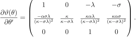
In Section 3, we consider a parameter transformation ϑ = (b, a, σ)′ _{= ϑ(θ) for both of the}

Vasicek and CIR models such that b = κ₋σλ and a = _κ−κα_σλ are the drift parameters under the risk neutral measure, which are more direct to the bond price. Let

∂ϑ(θ) ∂θ′ =



   

1 0 ₋λ ₋σ

−ασλ

(κ−σλ)2 _κ−κ_{σλ (κ−}καλ_σλ)2 _(κ−κασ_σλ)2

0 0 1 0



    .

According to Theorem 5.1 and the delta-method, the plug-in estimator ˆϑn(E, W) = ϑ (

ˆ

θn(E, W) )

is asymptotic normal in that

√

n(ϑˆn(E, W)−ϑ0

) _d

−→N (

0,∂ϑ(θ0) ∂θ′ Q

−1

0 (δ;E, W)

∂ϑ(θ0)′

∂θ )

.

Table 2 also reports the estimates of a and b under the risk neutral measure. It reveals that

despite the rather volatile estimates for the parameters under the physical measure, the parameter

the estimated λ may incur large errors, the estimates for parameters which directly influence the

bond pricing were more reliable.

Table 3 reports the estimated correlation matrix (standardized ˆVn(E1)) of the pricing errors

under the CIR model by using the maturity group of 1-5 years, which has been shown to fit

the CIR model quite well in Table 1. Before standardizing ˆVn(E1), we found that the estimated

standard deviations of the pricing errors were increasing along with the time to maturity almost

linearly. We observe from Table 3 that (i) the dependence in the pricing errors was quite persistent

with the correlation coefficients decaying very gradually as the gap between the maturities was

increased; and (ii) the correlations were consistently positive. The results reveal that it may be

too simplistic to specify a diagonal form forV0.

The sample covariance ˆVn(E1) has been used to estimate V0 ∈ RM×M to obtain the feasible

combined estimators in Table 2. Suggested by a referee, we implemented an alternative

covari-ance estimator suitable for high dimensions. Specifically, we consider the non-negative covaricovari-ance

estimator proposed in Rothman (2012). It is noted that although in our current setting the

dimen-sion M (the number of bonds) is fixed and is smaller than the sample size n, experimenting the

estimator of Rothman (2012) provides insights for higher dimensional situations. Denote

Roth-man (2012)’s covariance estimator as ¯Vn(E1) which was computed using an R package “PDSCE”.

The combined estimates for the CIR model based on ¯Vn(E1) are reported in the supplementary

material. The results also contain the spectral norm of ¯Vn(E1)−Vˆn(E1), which indicates the two

covariance estimators were generally close to each other. Comparing Table 2 with the combined

estimates based on ¯Vn(E1), we observe that although there were some differences in the parameter

estimates using the two covariance estimators, the differences were not significant when considered

in terms of the standard errors. And more importantly, the insights found in Table 2 as discussed

8

Conclusion

Despite the interest rate models are such basics in the modern financial theory and practice,

getting proper models and estimating their parameters have been challenging. A key aspect of

the challenge is rooted in the fact that the short (instantaneous) rates are not directly observable.

There have been two approaches to find approximations to the short rates. One is to use rates

with shorter maturities as proxies to the short rates, as adopted in Chan, Karolyi, Longstaff and

Sanders (1992), Nowman (1997), A¨ıt-Sahalia (1996) and A¨ıt-Sahalia (1999). The other approach,

which we call the implied state variable approach, is to calibrate the short rates via the bond

prices by assuming that one or a few bond prices follow exactly (2.5) without errors whereas

the other bonds are subject to errors; see Chen and Scott (1993), Duffee (2002), Cheridito et al.

(2007), A¨ıt-Sahalia and Kimmel (2010), Joslin, Singleton and Zhu (2011) and Hamilton and Wu

(2014). It is fair to say that both approaches use certain type of proxies to approximate the short

rates. Indeed, while the first approach assumes that there are quality proxies to the short rates,

the implied state variable approach assumes certain numbers of the bond prices are observed

accurately.

We use the first approach in our analysis in this paper. Although we used the over-night Fed

fund rates as proxies to the short rates in the case study, interest rates with other maturities can

be used to avoid the micro-structures of the over-night rates as noted in Filipovi´c (2009). For

instance, A¨ıt-Sahalia (1996) used the 7-day Eurodollar deposit spot rate, bid-ask midpoint as the

proxy of the short rate.

The proposed approach can be viewed as a further development of the bond return method used

in Brown and Dybvig (1986) and Gibbons and Ramaswamy (1993) by considering cross-sectional

prices of bonds as well as the conditional model information of the short rate processes. The

combination of the short rate dynamic information and the bond prices allows for enhancement

of estimation beyond the MLE based on the short rates only and identification of all parameters.

The proposed combined estimation is semiparametric with respect to the measurement errors.

error structure given our findings in the case study that the size of the pricing error was largely

influenced by the maturity, and that there was substantial dependence between errors of different

maturities. The dependence became larger as the time to maturity increased, which indicates

that it would be too simplistic to assume a diagonal form for V0 as assumed in some of the

implementation of the implied state variable approach. The proposed approach avoids directly

specifying the covariance structure of the pricing errors while still achieving good efficiency in the

estimation.

The reason why we focus on the time homogenous affine term structure modeling in this paper

is mainly driven by real applications of interest rates and bond prices (A¨ıt-Sahalia, 2002; Cheridito

et al., 2007; A¨ıt-Sahalia and Kimmel, 2010). Proposed by an anonymous referee, we discuss the

time inhomogeneous scenario in the following. The MLE discussed in Section 2 can be shown

to be asymptotically normal using the martingale convergence theorems (Hall and Heyde, 1980).

Based on the similar technics, we can show that

[

Var {

1 n

n ∑

t=1

ht(θ0;E, W)

}]−1/2 1 n

n ∑

t=1

ht(θ0;E, W)

is asymptotically normal if we impose the similar conditions of Assumptions 1 and 2 in Hall

and Heyde (1980, p. 160). Then our combined estimation approach can be carried out and

the asymptotic normality of the GMM estimator is still valid. However, the range of the time

inhomogeneous processes adapted to the conditions needs to be further investigated in the future

study.

We have considered in this paper one-factor models in our attempt to utilize the bond prices

to enhance the estimation of the parameters of the interest rate processes. Extensions may be

made to the multi-factor affine term structure models, which would require the filtering techniques

to be used. While we leave this extension to future consideration, we note that despite a set of

multi-factor models have been proposed, almost all these models are rejected in the empirical

A

Appendix: Technical Details

Throughout the appendix, we use ∆ to denote a finite positive constant, and denote the spectral

norm of a matrix A= (aij)q×p as∥A∥2 = √

λmax(A′A), where λmax(A′A) is the largest eigenvalue

of A′_{A, and the Frobenius norm ∥A∥ =} √

tr(A′_{A) =} √∑q i=1

∑p

j=1a2ij. For a stationary matrix process{Ft(θ) = (Fij,t(θ))_q×p

}

relying on a finite dimension vectorθ, wherepandqare also finite,

PnFt(θ) := _n1 ∑nt=1Ft(θ). For the first and second derivatives, ˙ℓt(β) := ∂ℓ_∂βt(β), ℓ¨t(β) := ∂

2_ℓ t(β)

∂β∂β′ ,

˙

A(θ) := ∂A_∂θ(θ′),B˙(θ) :=

∂B(θ)

∂θ′ and ˙ht(θ) :=

∂ht(θ)

∂θ′ . We suppress the expressionE and W in ¯θn(E, W)

and ht(θ;E, W), and write them as ¯θn and ht(θ) whenever doing so would not cause confusion. We firstly present the assumptions needed in our analysis. Assumptions used for the

approx-imate MLE of A¨ıt-Sahalia (1999, 2002) are presented as well, as we have used an approach that

can lead to results for both the combined estimation using either the full likelihood scores or the

approximated likelihood scores. Discussions to the assumptions including comparison with the

conditions in the extant literatures are given in the supplementary material.

Assumption 1. (i) θ = (β′_{, λ}′₎′ _{= (θ}

1,· · · , θq+d)′ ∈ Θ which is a compact set in Rq+d, where β = (β1,· · · , βq)′ ∈ B ⊂Rq. (ii) The true value θ0 ∈Θ is an interior point. (iii) β0 is the unique

root ofE{∂ℓt(β)

∂β }

= 0 for every δ. (iv) θ0 is the unique root of E{ht(θ;Iq+d, W)}= 0 for every δ.

Assumption 2. (i) The short rate r(t) follows the time homogeneous diffusion processes (2.1)

and (2.3) under measuresQ0andQ1. Assumption 1 in A¨ıt-Sahalia and Mykland (2004) is satisfied

under the measure Q0, and (2.4) holds under the measureQ1. (ii) The pricing functions in (2.6)

and (2.7) are three times differentiable with respect toθ. (iii) For fixedτ1,· · · , τM and fixedM, the time homogeneous pricing functions A(θ) = (A1(θ),· · · , AM(θ))′ and B(θ) = (B1(θ),· · · , BM(θ))′ satisfy

sup θ∈Θ|

Ai(θ)| ≤M1,sup

θ∈Θ|

Bi(θ)| ≤M1,sup

θ∈Θ

∂l_A i(θ) ∂θj1· · ·∂θjl

≤

M1 and sup

θ∈Θ

∂l_B i(θ) ∂θj1· · ·∂θjl

≤

M1,

for a fixed positive constant M1 > 0 and any i = 1,2,· · · , M, l = 1,2,3 and j1, j2, j3 ∈ {1,2,_{· · ·} , q+d_}.

Assumption 3. (i)_∂β∂ ∫

f(rt|rt−1, δ;β)drt = ∫ _∂

∂βf(rt|rt−1, δ;β)drtand ∂ ∂β

∫ _∂

∫ _∂2

∂β∂β′f(rt|rt−1, δ;β)drt, which imply the Fisher information matrix E {

−∂2ℓt(β0)

∂β∂β′

}

=: _I0(δ). (ii)

For any nonrandom δ >0, _I0(δ) is invertible and

δ

1/2_I−1/2 0 (δ)

2 =O(1).

Assumption 4. The J-term expansion to the log of transition density ℓt(β) in (2.2) is

ℓ(_tJ)(β) = ₋log√2πδ+_A1(rt|rt−1, δ;β) +A2(rt|rt−1, δ;β) +A3(J)(rt|rt−1, δ;β), (A.1)

where _A(₃J)(x_|x0, δ;β) = log

{ ∑J

j=0cj(γ(x;β)|γ(x0;β);β)

δj

j!

}

for J _≥ 1, and the expressions of the functions _A1,_A2, γ and cj can be found in A¨ıt-Sahalia (1999). Let

h(_tJ)(θ;_E, W) = 



∂ℓ(tJ)(β)

∂β

E′_g

t(θ;W) 

 (A.2)

as a approximate forht(θ;E, W) in (4.1) to establish our proposed estimator. Assumptions (A.3), (A.6) and (A.7) in Chang and Chen (2011) hold and there exist finite positive constants νk for

k = 0,1,2,3, and M2 such that ν0 > 3, ν2 > ν1 > 3, ν3 > 1 and for any i1,· · · , i3 ∈ {1,· · · , q},

δ_∈(0,∆],

E  sup β∈B { _∞ ∑ l=0

∂k_c

l(γ(rt;β)|γ(rt−1;β);β)

∂βi1· · ·∂βik

δl l!

}2νk

≤M2. (A.3)

Assumption 5. (i) The measurement error _{u0t} in (3.2) is a martingale difference array with respect to the filtration_{Gt}, whereGtis theσ-algebra generated by{(rl+1, u′0l)′}l≤t. (ii) The short rate and measurement error process _{(rt, u′0t)′} is stationary and satisfies (3.1). (iii) We assume

{(rt, u′0t)′} is ρ-mixing with the ρ-mixing coefficient ρ(k) := sup

Z1∈L2(F−∞0 ),Z2∈L2(Fk+∞)

|Corr(Z1, Z2)| ≤C1e−C2k, (A.4)

where_F0

−∞is theσ-algebra generated by{(rl, u0′l)′}l≤0,F

∞

k is theσ-algebra generated by{(rl, u′0l)′}l≥k, and C1, C2 are positive constants. (iv) E(r4t) <∞ and E(u40it) <∞. (v) E(u0tu′0t|Gt−1) =:V0 =

(vjk)M×M is of full rank and W is an M ×M nonrandom positive definite matrix.

Assumption 6. (i) q†

≥ d. (ii) Based on the definition of _E in (4.4), there exists a q†

×(q+d) nonrandom matrixZ(θ0) which depends only on θ0 and τ1· · · , τM, such that

The q†

×d matrix Zλ(θ0) :=Z(θ0)(0d×q, Id)′ satisfies rank{Zλ(θ0)}=d.

In the following we present the lemmas as well as the proofs of the propositions and theorems by

using these lemmas. The proofs of the lemmas and some corollaries are left in the supplementary

material.

Lemma A.1. Under Assumptions 1, 2, 4 and 5, there exist positive constants M01, M02 < ∞

and ∆1, such that for any J, where J can be infinity, l = 1,2, δ ∈ (0,∆1], d ≤ K ≤ q+d, and

i1, i2 ∈ {1,2,· · · , q+d}, j ∈ {1,2,· · · , q+K},

E

{ sup θ∈Θ

h

(J)

tj (θ)

2}

≤M01∨M02 and E

 

 sup θ∈Θ

∂l_h(J)

tj (θ) ∂θi1· · ·∂θil

2  

≤M01∨M02,

where h(_tj∞)(θ) = htj(θ), ∂l_h(∞)

tj (θ)

∂θi₁···∂θ_il =

∂l_h tj(θ)

∂θi₁···∂θ_il and h

(J)

t (θ) = (

h_t(J₁)(θ),_{· · ·} , h_t(₍J_q)_+K)(θ))′.

Lemma A.2. For every i, j, there exists a constant M31 such that E

{

sup_θ∈Θ

∂Fij,t(θ)

∂θk

}

≤M31< ∞ for every component θk of vector θ. Besides, for each θ ∈ Θ, PnFij,t(θ)−E{Fij,t(θ)}

p

−→ 0. Then sup_θ∈Θ∥PnFt(θ)−E{Ft(θ)}∥2

p

−→0 as n_{→ ∞}.

Lemma A.3. Under Assumptions 1, 2 and 4,

Pnℓ˙t(β)−E {

˙ ℓt(β)

} =Op

(

(nδ)−1/2)

for each β _{∈ B} and sup

β∈B

Pn

˙

ℓt(β)−E {

˙ ℓt(β)

}

2

p

−→0,

for δ_∈(0,∆1], n→ ∞.

Proof of Proposition 4.1: According to the stationary, (A.4) and Lemma A.1, by Theorem

16.3.8 in Athreya and Lahiri (2006), the long-run covariance matrix limn→∞nVar{Pnht(θ0)} =

Γ(0) +∑∞

k=1{Γ(k) + Γ(k)′} converges, where

Γ(k) =_E 

 ˙

ℓt(β0) ˙ℓt−k(β0)′ ℓ˙t(β0)gt−k(θ0;W)′E E′_g

t(θ0;W) ˙ℓt−k(β0)′ E′gt(θ0;W)gt−k(θ0;W)′E



.

It is worth noting that we have E{gt(θ0;W)

G_t−1

}

= 0 by Assumption 5. Then the proposition

Lemma A.4. Under Assumptions 3, 5 and 6,Ω(δ;_E, W)defined in (5.3) and _Q0(δ;E, W)defined

in (5.2) are invertible for any δ_∈(0,∆1], and

δ

1/2_Q−1/2

0 (δ;E, W)

2 =O(1).

Proof of Theorem 5.1: Let W _{= diag}{

I0−1(δ),Ξ

−1 0

}

. Taking the Taylor expansion at θ0 on the

first oder condition to the minimization,{_Pnh˙t(θ0)

}′ ˆ

W_{n{Pnht(θ0)}+Qn}(_θˆ_n−θ0)_{= 0 and}

Qn :=Q(ˆθ) := {

Pnh˙t(ˆθ) }′

ˆ

W_n{_Pnh˙_t(ˆθ)}₊

[ {

Pnht(ˆθ) }′

ˆ

W_n⊗Iq+d

] 

Pn

∂ vec {h˙t(ˆθ)′ }

∂θ′



, (A.6)

where ˆθ =θ0+zn(ˆθn−θ0) and 0≤zn≤1. Then according to Lemma A.1 and Lemma A.3,

−√n_Q1₀/2(δ)(θˆn−θ0

)

=√n_Q−₀1/2(δ){Pnh˙t(θ0)

}′ ˆ

W_n{Pnht(θ0)}

+_Q−₀1/2(δ)_{Qn− Q0(δ)} Q−01/2(δ)

{√

n_Q1₀/2(δ)(θˆn−θ0

)}

= √nPnQ−01/2(δ)H0(δ)′Wht(θ0) +op (

√

n_Q1₀/2(δ)(ˆθn−θ0)

2

)

+op(1) d

−→N(0, Iq+d) since E

Q

−1/2

0 (δ)H0(δ)′Wht(θ0)

2

=q+d <_∞, the long-run covariance matrix lim

n→∞nVar

{

PnQ−01/2(δ)H0(δ)′W ht(θ0)

}

=Iq+d

by Proposition 4.1, the stationarity, (A.4) and Theorem 16.3.8 in Athreya and Lahiri (2006). □

Proof of Theorem 5.2: Note thatψ(θ0)E1 andψ(θ0)E2are both of full rank. From (A.5), we have

ψ(θ0) =ψ(θ0)E1Z1(θ0) = ψ(θ0)E2Z2(θ0), namely the columns of the matrices ψ(θ0)E1 and ψ(θ0)E2

form a basis to the columns ofψ(θ0). Then there exists a full rank nonrandomq†×q†matrixZ(θ0)

such thatψ(θ0)E1 =ψ(θ0)E2Z(θ0). Hence, by (5.2) we have Q0(δ;E1, W) =





I0(δ) 0q×d 0d×q 0d×d



+

Z1(θ0)′{E1′ψ(θ0)′(I2⊗W)ψ(θ0)E1} {E1′ψ(θ0)′[I2⊗(W V0W)]ψ(θ0)E1}−1{E1′ψ(θ0)′(I2⊗W)ψ(θ0)E1}Z1(θ0)

=Q0(δ;E2, W) considering the invertible Z(θ0). Then the theorem is proved by Theorem 5.1. □

Acknowledgements: We thank the Editor, the AE and two referees for helpful comments and

suggestions which have improved the presentation of the paper. The research was partially

References

A¨ıt-Sahalia, Y. (1996). Testing continuous-time models of the spot interest rate. Review of

Financial Studies, 2, 385–426.

A¨ıt-Sahalia, Y. (1999). Transition densities for interest rate and other nonlinear diffusions. The

Journal of Finance, 54, 1361–1395.

A¨ıt-Sahalia, Y. (2002). Maximum likelihood estimation of discretely sampled diffusions: A closed-form approximation approach. Econometrica, 70, 223–262.

A¨ıt-Sahalia, Y. and Kimmel, R. (2007). Maximum likelihood estimation of stochastic volatility models. Journal of Financial Economics, 83, 413–452.

A¨ıt-Sahalia, Y. and Kimmel, R. L. (2010). Estimating affine multifactor term structure models using closed-form likelihood expansions. Journal of Financial Economics, 98, 113–144.

A¨ıt-Sahalia, Y. and Mykland, P. A. (2004). Estimators of diffusions with randomly spaced discrete observations: A general theory. The Annals of Statistics, 32, 2186–2222.

Athreya, K. B. and Lahiri, S. N. (2006). Measure Theory and Probability Theory. Springer Verlag.

Brigo, D. and Mercurio, F. (2006). Interest Rate Models: Theory and Practice. Springer Verlag.

Brown, S. J. and Dybvig, P. H. (1986). The empirical implications of the Cox, Ingersoll, Ross theory of the term structure of interest rates. The Journal of Finance, 41, 617–630.

Chan, K. C., Karolyi, G. A., Longstaff, F. A., and Sanders, A. B. (1992). An empirical comparison of alternative models of the short-term interest rate. The Journal of Finance, 47, 1209–1227.

Chang, J. and Chen, S. X. (2011). On the approximate maximum likelihood estimation for diffusion processes. The Annals of Statistics, 39, 2820–2851.

Chen, R.-R. and Scott, L. (1993). Maximum likelihood estimation for a multifactor equilibrium model of the term structure of interest rates. The Journal of Fixed Income, 3, 14–31.

Chen, S. X., Gao, J., and Tang, C. Y. (2008). A test for model specification of diffusion processes.

The Annals of Statistics, 36, 167–198.

Cheridito, P., Filipovi´c, D., and Kimmel, R. L. (2007). Market price of risk specifications for affine models: Theory and evidence. Journal of Financial Economics, 83, 123–170.

Cox, J. C., Ingersoll Jr, J. E., and Ross, S. A. (1985). A theory of the term structure of interest rates. Econometrica, 53, 385–407.

Dai, Q. and Singleton, K. J. (2000). Specification analysis of affine term structure models. The

Journal of Finance, 55, 1943–1978.

Duffee, G. R. (2002). Term premia and interest rate forecasts in affine models. The Journal of

Finance, 57, 405–443.

Duffie, D. and Kan, R. (1996). A yield-factor model of interest rates. Mathematical Finance, 6, 379–406.

Fama, E. F. (1976). Forward rates as predictors of future spot rates. Journal of Financial

Economics, 3, 361–377.

Feller, W. (1951). Two singular diffusion problems. The Annals of Mathematics, 54, 173–182.

Filipovi´c, D. (2009). Term-Structure Models: A Graduate Course. Springer Verlag.

Gibbons, M. R. and Ramaswamy, K. (1993). A test of the Cox, Ingersoll, and Ross model of the term structure. Review of Financial Studies, 6, 619–658.

G¨urkaynak, R. S., Sack, B., and Wright, J. H. (2007). The US treasury yield curve: 1961 to the present. Journal of Monetary Economics, 54, 2291–2304.

Hairer, E., Nøersett, S. P., and Wanner, G. (2006). Solving Ordinary Differential Equations. Springer Verlag.

Hall, P. and Heyde, C. C. (1980). Martingale Limit Theory and Its Application. Academic Press, New York.

Hamilton, J. D. and Wu, J. C. (2014). Testable implications of affine term structure models.

Journal of Econometrics, 178, 231–242.

Hansen, L. P. (1982). Large sample properties of generalized method of moments estimators.

Econometrica, 50, 1029–1054.

Hull, J. (2009). Options, Futures, and Other Derivatives. Pearson.

Joslin, S., Singleton, K. J., and Zhu, H. (2011). A new perspective on Gaussian dynamic term structure models. Review of Financial Studies, 24, 926–970.

Langetieg, T. C. (1980). A multivariate model of the term structure. The Journal of Finance, 35, 71–97.

McCulloch, J. H.and Kwon, H.-C. (1993). U.S. term structure data, 1947-1991. Ohio State

Working Paper, 93–6.

McCulloch, J. H. (1975). The tax-adjusted yield curve. The Journal of Finance, 30, 811–830.

Nelson, C. R. and Siegel, A. F. (1987). Parsimonious modeling of yield curves.Journal of Business, 60, 473–489.

Nowman, K. B. (1997). Gaussian estimation of single-factor continuous time models of the term structure of interest rates. The Journal of Finance, 52, 1695–1706.

Pearson, N. D. and Sun, T.-S. (1994). Exploiting the conditional density in estimating the term structure: An application to the Cox, Ingersoll, and Ross model. The Journal of Finance, 49, 1279–1304.

Rothman, A. J. (2012). Positive definite estimators of large covariance matrices. Biometrika, 99, 733–740.

Svensson, L. E. O. (1994). Estimating and interpreting forward rates: Sweden 1992-4. National

Bureau of Economic Research Working Paper, page 4871.

Tang, C. Y. and Chen, S. X. (2009). Parameter estimation and bias correction for diffusion processes. Journal of Econometrics, 149, 65–81.

Vasicek, O. (1977). An equilibrium characterization of the term structure. Journal of Financial

Economics, 5, 177–188.

Vasicek, O. A. and Fong, H. G. (1982). Term structure modeling using exponential splines. The

Journal of Finance, 37, 339–348.

Table 1: J-tests for the Vasicek and CIR models based on the Federal fund rates and bond prices.

GMM: _E1 = (e2, e3, e4) (Moment Conditions I)

1₋3 1₋5 1₋10 1₋15 6₋15 Vasicek J-statistic 10.2720 30.8105 11.4163 30.6171 32.3894

p-value 0.0059 0.0000 0.0033 0.0000 0.0000

CIR J-statistic 0.8903 1.4591 9.0660 26.4127 28.3110

p-value 0.6407 0.4821 0.0107 0.0000 0.0000

GMM: _E2 = (e1, e2, e3) (Moment Conditions II)

1₋3 1₋5 1₋10 1₋15 6₋15 Vasicek J-statistic 10.3928 10.0876 6.8914 7.9270 7.9914

p-value 0.0055 0.0064 0.0319 0.0190 0.0184

CIR J-statistic 0.7671 1.4826 11.4109 48.9833 50.4626

Table 2: Combined estimates based on the monthly Federal fund rates and bond prices for the

CIR model (W = ˆV−1

n (E1)). Figures inside the parentheses are the standard errors of the estimates

above.

MLE 1₋3 1₋5 1₋10 1₋15 6₋15

κ 0.1875 0.1705 0.1635 0.2454 0.1504 0.1836

(0.0337) (0.0239) (0.0243) (0.0331) (0.0295) (0.0295)

α 0.0751 0.0645 0.0696 0.0574 0.0857 0.0726

(0.0133) (0.0090) (0.0103) (0.0077) (0.0167) (0.0117)

σ 0.0641 0.0544 0.0548 0.0647 0.0604 0.0607

(0.0007) (0.0004) (0.0004) (0.0007) (0.0005) (0.0005)

λ - 0.6589 0.4772 1.2344 0.0608 0.5713

- (0.4390) (0.4417) (0.5127) (0.4867) (0.4866)

b - 0.1347 0.1374 0.1655 0.1467 0.1489

- (0.0058) (0.0054) (0.0046) (0.0043) (0.0043)

a - 0.0817 0.0829 0.0852 0.0878 0.0895

- (0.0015) (0.0010) (0.0009) (0.0010) (0.0010)

Table 3: Estimated correlation matrix of the measurement errors for 1-5 years maturity under

the CIR model.

τ_i 2 3 4 5

1 0.950 0.879 0.811 0.749

2 0.983 0.949 0.911

3 0.991 0.971

500 1000 1500 2000

0.05

0.15

0.25

0.35

W=I

n

SD of

κ

MLE M=5, MC I M=5, MC II M=15, MC I M=15, MC II

500 1000 1500 2000

0.05

0.15

0.25

0.35

W=V

^

−1

n

SD of

κ

MLE M=5, MC I M=5, MC II M=15, MC I M=15, MC II

500 1000 1500 2000

0.004

0.008

0.012

W=I

n

SD of

α

MLE M=5, MC I M=5, MC II M=15, MC I M=15, MC II

500 1000 1500 2000

0.004

0.008

0.012

W=V

^

−1

n

SD of

α

MLE M=5, MC I M=5, MC II M=15, MC I M=15, MC II

Figure 1: Simulated standard deviation (SD) of the MLEs ( ˜βn), and the combined estimators (ˆθn)

with two moment selection matrices_E1 (MC I) andE2 (MC II) forκandα in the CIR model with

500 1000 1500 2000

0.002

0.004

0.006

0.008

W=I

n

SD of

σ

MLE M=5, MC I M=5, MC II M=15, MC I M=15, MC II

500 1000 1500 2000

0.002

0.004

0.006

0.008

W=V

^

−1

n

SD of

σ

MLE M=5, MC I M=5, MC II M=15, MC I M=15, MC II

500 1000 1500 2000

0.2

0.3

0.4

0.5

0.6

0.7

W=I

n

SD of

λ

M=5, MC I M=5, MC II M=15, MC I M=15, MC II

500 1000 1500 2000

0.2

0.3

0.4

0.5

0.6

0.7

W=V

^

−1

n

SD of

λ

M=5, MC I M=5, MC II M=15, MC I M=15, MC II

Figure 2: Simulated standard deviation (SD) of the MLEs ( ˜βn), and the combined estimators (ˆθn)

with two moment selection matrices_E1 (MC I) andE2 (MC II) forσ andλ in the CIR model with

500 1000 1500 2000

0.00

0.10

0.20

W=I

n

BIAS of

κ

MLE M=5, MC I M=5, MC II M=15, MC I M=15, MC II

500 1000 1500 2000

0.00

0.10

0.20

W=V

^

−1

n

BIAS of

κ

MLE M=5, MC I M=5, MC II M=15, MC I M=15, MC II

500 1000 1500 2000

0.00

0.10

0.20

0.30

W=I

n

BIAS of

λ

M=5, MC I M=5, MC II M=15, MC I M=15, MC II

500 1000 1500 2000

0.00

0.10

0.20

0.30

W=V

^

−1

n

BIAS of

λ

M=5, MC I M=5, MC II M=15, MC I M=15, MC II

Figure 3: Averaged absolute bias (BIAS) of the MLEs ( ˜βn), and the combined estimators (ˆθn)

with two moment selection matrices_E1 (MC I) andE2 (MC II) forκ andλ in the CIR model with