Automated spike sorting algorithm based on laplacian
eigenmaps and
k
-means clustering
E Chah1,2 , V Hok2 , A Della-Chiesa2, J J H Miller 3, S M O’Mara2 and R B Reilly1,2
1
Trinity Centre for Bioengineering, Trinity College, Dublin, Republic of Ireland 2
Trinity College Institute for Neuroscience, Trinity College, Dublin, Republic of Ireland
3
Department of Mathematics, Trinity College Dublin, Republic of Ireland E-mail: [email protected], [email protected], [email protected], [email protected] [email protected], [email protected]
Abstract
This study presents a new automatic spike sorting method based on feature extraction by Laplacian eigenmaps combined with k-means clustering. The performance of the proposed method was compared against previously reported algorithms such as principal component analysis (PCA) and amplitude-based feature extraction. Two types of classifier (namely k-means and classification expectation-maximization) were incorporated within the spike sorting algorithms, in order to find a suitable classifier for the feature sets. Simulated data sets and in-vivo tetrode multichannel recordings were employed to assess the performance of the spike sorting algorithms. The results show that the proposed algorithm yields significantly improved performance with mean sorting accuracy of 73% and sorting error of 10% compared to Principal Component Analysis which combined with k-means had a sorting accuracy of 58% and sorting error of 10%.
PACS: 87.19.L-Neuroscience, 87.85.Ng Biological signal processing 87.18.sn Neural networks and synaptic communication.
Submitted to: Journal of Neural Engineering.
Keywords: Automatic spike sorting, Laplacian eigenmaps, Action potential, Feature extraction, k-means clustering
1. Introduction
used in extracellular recordings may vary from single wire, tetrode (four wires twisted together) to microelectrode arrays configurations.
Though the electrodes’ configuration can differ from one experiment to another, the basic principle behind action potential sampling remains the same. Electrodes measure electric potential fluctuations in the extracellular space. These fluctuations generally contain two types of activity, low frequency content, also known as Local Field Potentials (LFPs) and extracellular action potentials (spikes) which contribute to the higher frequency content [2]. The spikes recorded by the electrodes represent spike events generated by an unknown number of neurons. The role of spike sorting is therefore to assign each spike to the neuron that produced it [3]. As the technology progresses multi-electrode arrays are increasingly being employed [4, 5]. Increasing the number of recording electrodes raises the need for automatic sorting, as manual sorting or human supervised sorting becomes a time consuming and tedious task.
The complexity of spike sorting can be attributed to several factors. It has been reported that spike waveforms for a given neuron can vary [6]; for example, during a complex spike burst, the amplitude of the spike can decrease by up to 80% [7]. Overlapping spikes create another complication when it comes to spike sorting; this phenomenon occurs when two or more closely spaced neurons fire action potentials simultaneously. Moreover, in the course of the recording session, the electrode may move slightly within the brain tissue due to external physical constraints, causing the spike waveform to vary in time [8].
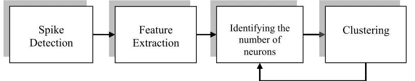
[image:2.612.92.499.385.465.2]Spike sorting algorithms – are typically composed of four steps in total (Figure 1). The first step involves detecting spike segments. The second step consists of extracting features that best discriminate the spikes produced by the different neurons. In the third step the number of neurons is estimated and often this step is carried in conjunction with final step. In the final step each spike is assigned to the neuron that generated it.
Figure 1. Illustration of the steps involved in spike sorting.
Spike detection methods reported in the literature include amplitude thresholding [9-11], and nonlinear energy operator [12, 13]. In the feature extraction step, parameters are computed from the spike that yields the best discrimination. The clustering step then groups the spikes with similar features together. In the literature, feature extraction methods range from simple approaches such as extracting peak-to-peak amplitude and width of the spike, to more advanced methods such as principal component analysis (PCA) [8] which is widely used [14-17]. Harris et al. [14] employed PCA features in conjunction with Bayesian classification (AutoClass) [18]. In [15] template matching was employed to achieve spike labelling. A combination of wavelet transform and k-means clustering was employed in [19]. Wavelet transform alongside superparamagnetic clustering was reported in [9]. In [20] Independent Component Analysis (ICA) and k-means clustering were employed. Waveform derivates with evolving mean shift clustering algorithm was proposed in [13]. In the literature a variety of methods are proposed to improve spike sorting algorithms. Improvement in spike sorting algorithms allows the isolation of larger number of spike clusters, hence maximizing the information extracted from in-vivo spike recordings.
In this study a robust method of automatic spike sorting is proposed based on Laplacian eigenmaps feature extraction combined with the k-means clustering algorithm. The performance
Clustering Feature
Extraction
Identifying the number of
neurons Spike
of the proposed method is compared with systems based on simple amplitude features and on PCA derived features. Two types of classification algorithms were employed in this study, namely k-means and classification expectation-maximization algorithms (CEM, as implemented in KlustaKwik [21] ).
2. Data set
Simulated data used in this study were obtained from the publicly available data set Wave_clus [9]. Eight simulated recordings (named A-H in Table 1) were employed in this study, including simulations of complex spike cells (data set B) and electrode drift (data set D). All simulated data sets in our study included overlapping spikes. On average, the percentage of overlapping spikes accounts for 20% of the overall spike population. Each file contains spikes from three neurons. The average number of neural spikes in the files was ~ 3450. Standard deviation of noise in the data set varied between 5% - 20% of the spike peak amplitude. The noise was constructed to simulate background neural activity. This was achieved by adding average spike waveforms at random times and with random amplitudes to form the noise signal. The simulated data spike clusters had a mean firing rate of 20 Hz and a 2 ms refractory period.
Simulated data has the advantage of being objective and it provides an error-free benchmark. However, it has several shortcomings. For example, the simulated data represents a single channel recording. However it has been established that multichannel recording such as tetrodes markedly improve spike sorting [22]. Hence, it is vital to consider multichannel recording when assessing the performance of spike sorting algorithms.
The simulated data sets in this study contained spikes from three neurons in each recording, however when it comes to in-vivo studies, more neurons may be recorded by each channel. Theoretical estimations suggest that a tetrode can sense spikes from ~ 140 neurons with sufficient spike amplitude for spike sorting [23]. In practice, however, the number of neurons sensed will be fewer ~20 [23]. A higher number of clusters can lead to lower classification accuracy. For example, if there are two clusters, the probability of classifying an object correctly by chance is 50%, while if the number of clusters increase to 10, the probability is reduced to 10%.
To address the shortcomings of the simulated data set, we have also evaluated the performance of spike sorting algorithms on in-vivo recording from the hippocampus of a freely moving rodent. A surgical procedure was followed for the implantation of electrodes; the animal was anaesthetized with isofluorane and mounted on a sterotaxic frame for precise positioning of the electrodes (see [24] for further details). The animal was allowed to freely explore an enclosure for 20 min during the recording. Experiments were conducted in accordance with European Community directive, 86⁄609⁄EC, and the Cruelty to Animals Act, 1876, and followed Bioresources Ethics Committee, Trinity College, Dublin, Ireland, and international guidelines of good practice.
The in-vivo data was collected using a commercial spike recording system (Axona, Ltd.). The recording was obtained using a tetrode configuration with one channel set as a reference. In this case, the results of automatic sorting were compared against expert manual sorting. The expert was able to sort and reliably isolate spikes of two neurons (~ 3890 spikes). The remaining detected segments were considered as noise event. The total number segments detected (noise and spikes) was ~ 10400. Manual spike sorting was carried out offline using graphical cluster-cutting software (Axona, Ltd.). The spike sorting performance using in-vivo data provides an insight into the performance of the spike sorting algorithms for practical spike sorting by the scientific community.
3. Methods
Spike sorting involves four steps (See Figure 1) as follows:
The spike detection employed in this study was based on the method reported in [9]. The recordings were high-pass filtered (300 Hz). The background noise standard deviation was estimated using the formula below:
6745 . 0
) ( f noise
x median
(1)
Where xf refers to the sampled filtered signal. The threshold was chosen as in [9] to be4noise. Spikes are detected when this threshold is exceeded. Each detected spike is represented by 64 samples when the threshold was exceeded. This corresponds to ~ 2.7 ms.
3.2. Feature extraction
Feature sets were divided into three categories:
3.2.1. Laplacian eigenmaps. Laplacian eigenmaps (LE) is a dimension reduction method [25]. As with any data reduction method, the problem is that given a set of x1, ... ,xM of M points in R
l , find a set of point y1, ... , yM in R
n
(n<<l) such that yi represents xi. The objective of Laplacian eigenmaps is to map points which are found to be similar under a specific definition, to points close together [25, 26]. Let y = (y1,y2,y3, … ,ym)
T
be such a map, this objective is achieved by minimizing the following function:
2
) (yiyj
ijWij (2)Where Wij is defined in eq. (3). This weight function (Wij) ensures that points close to each other assigned a large weight while points further apart assigned a smaller weight. Since this function decreases exponentially, points mapped further apart incur a heavier penalty [25]. These mappings demonstrate the potential suitability of LE in spike sorting algorithms. For a detected spike segment x of length M the LE algorithm has the following steps:
First step: The Euclidean distance matrix is computed ||xi – xj|| 2
. Then n nearest neighbours are connected. i.e. if node j is among the n nearest neighbours of i then nodes i and j are connected.
Second step: Weight matrix is computed according to eq. (3).
otherwise
connected are
j and i if e
Wij
0
2 2
j i x x
(3)
Third step: for the connected component the generalized eigenvalues and eigenvectors are computed.
Lf = Df
Where is the eigenvalue and f is the corresponding eigenvector
(4)
With Dii
jWij (5)Laplacian matrix LDW (6)
Forth Step: The eigenvectors are sorted according to their eigenvalues:
m 2
1 0
Final Step: The mapping of xi into the lower m dimension space is then given by (f1(i), … , fm(i)). Ignoring the first eigenvector f0 which corresponds to the eigenvalue 0. There are two parameters to be determined in the Laplacian eigenmap dimension reduction algorithm, namely n and. It is reported in [27, 28] that choosing n values between (5 - 21) is sufficient for spike cluster separation. In this study n = 12 was chosen which is in the range reported in the literature. was determined empirically; higher values than 0.6 were shown to have no effect in improving the cluster separation. In this studywas set to a simple value of 1. The dimension of the features extracted from the spikes using Laplacian eigenmaps dimension reduction was limited to three dimensions, in line with the other feature extraction methods compared in this study.
3.2.2. PCA features. Principal Component Analysis (PCA) finds a set of orthogonal basis vectors that represent the largest variation of the data. It has been reported for spike sorting that choosing the first three principal components provides good separation [29]. Choosing a higher number of components would account for higher variation; however, higher components were found to be dominated by background noise [8]. In this study the PCA features consisted of the first three PCA components.
3.2.3. Amplitude-Only features. Amplitude-only features were based on the temporal characteristic of the spike waveform. The distance between the neuron and electrode is an important factor in determining the amplitude sensed by the electrode [23, 30]. In an environment where neurons are not equidistant with respect to the electrode, the amplitude of the spikes can be used to discriminate spikes from different neurons.
The temporal characteristics extracted included:
The positive peak amplitude of the spike.
The amplitude of the local minimum before the peak.
The amplitude of the local minimum after the peak.
3.3. Clustering
Two types of clustering algorithms were used in this study:
3.3.1. k-means clustering. k-means clustering [31] is a simple clustering algorithm involving few steps, although the number of clusters k must be predetermined. In spike sorting methods, the number of neurons contributing to the spikes sensed by the electrode is not known, and therefore, it is not possible to preset k. To overcome this k-means limitation the PBM index [32] was employed to determine k. The PBM index is a cluster validity index; it measures the “goodness” of clustering using a range of clusters (k).
Below is a short description of the steps in k-means combined with PBM index algorithms:
Step1: number of clusters is initially set to k.
Step2: k points are chosen randomly in the feature space as the initial cluster centres CCj where j = 1,… , k.
Step 3: For a feature vector A of length N, find the Euclidean distance between each Ai and CCj, j=1,… ,k, where i= 1,… , N.
Step 4: Assign Ai to the cluster CCj which gives the minimum Euclidean distance. Step 5: Recalculate cluster centres CCj using the points in each cluster.
The steps 2-5 are repeated until no change is obtained, below a certain threshold, in cluster centres CCj. In practice clustering is repeated a number times with different initial random cluster centres so that a local minimum is not interpreted as the optimum classification result.
2 k k 1 S E E k 1 k PBM ) ( (8)
Where k is the number of clusters, Sk is the maximum separation between cluster centres; E1 is the sum of separation between the points and the cluster centres when number clusters k =1. Ek is the sum of separations between the feature points and the k cluster centres.
Step 7: Choose k that yields the highest PBM index.
3.3.2. Classification expectation-maximization. We used the software KlustaKwik which is based on the Classification Expectation-Maximization algorithm (CEM) [33].
4. Performance measure metrics
Two metrics were used to evaluate the performance of the spike sorting system. Similar to [13] a classification matrix (CM) was computed. However, a modified matrix was developed to include the “noise events” or non-spike events.
kK 3 k 2 k 1 k 0 k K 3 3 32 31 30 K 2 23 2 21 20 K 1 13 12 1 10 k 3 2 1 K 3 2 1 0 FP FP FP FP FP FP TP FP FP FP FP FP TP FP FP FP FP FP TP FP C C C C CM N N N N N (9)
Where N0 refers to noise events, and N1 N2 N3 ... NK reflect the spikes produced by each neuron respectively, C1, C2 and C3 ...Ck refer to the clusters identified by the spike sorting method. K refers to the actual number of neurons in the recording, k refers to the number of clusters identified. TPi is the number of spikes from neuron i in the cluster i (true positives). FPij is the number of spikes from neuron j in the cluster i (False positives), note that j = 0 corresponds to noise events.
The first measure of performance is the Sorting Accuracy (SA) which is the percentage of the detected spikes labelled correctly:
K i k j i j i ij i K i i FP TP TP SA1 , 1,
1
100
(%) (10)
Sorting Error SE is the ratio between the false positives and the total number of segments (spikes and noise) in identified clusters.
K i K j i j i ij i K j i j i ij FP TP FP SE1 1, 0, , 0 , 1 100 (%) (11)
A perfect spike sorting algorithm will yield a SA of 100 % and SE 0 % which corresponds to
ik0,j1,ijFPij 0 .5.1. Spike detection:
The performance of the spike detection method was assessed based on the percentage of neural spikes detected correctly. In this study mean percentage of neural spikes detected was 92% with a standard deviation of 10%. The percentage noise events is defined as the ratio between noise events and total number of segments detected (noise and neural spikes). The mean noise percentage was 2% and the standard deviation was 4%.
5.2. Spike sorting using simulated data set:
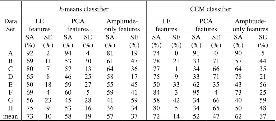
[image:7.612.85.529.241.436.2]The three feature extraction processes mentioned in the previous section were applied to the simulated data set and both types of classifiers were used to cluster the feature data. The results are shown in Table 1.
Table 1. Simulated data set results.
Data Set
k-means classifier CEM classifier
LE features
PCA features
Amplitude-only features
LE features
PCA features
Amplitude- only features SA
(%) SE (%)
SA (%)
SE (%)
SA (%)
SE (%)
SA (%)
SE (%)
SA (%)
SE (%)
SA (%)
SE (%)
A 92 2 94 4 81 19 74 0 91 0 90 5
B 69 11 53 30 61 47 78 21 33 71 57 44
C 80 7 57 13 64 36 77 1 34 66 64 35
D 65 8 46 25 58 17 75 9 33 71 78 21
E 80 18 59 27 55 45 50 33 62 35 43 56
F 69 4 60 5 59 41 84 3 95 4 73 25
G 56 23 45 28 41 59 58 42 34 66 40 59
H 75 9 53 16 36 34 80 5 34 65 50 48
mean 73 10 58 19 57 37 72 14 52 47 62 37
Comparing the mean performance metrics in the last row of Table 1, it is evident that LE combined with k-means classification yields higher sorting accuracy and lower sorting error percentages than other methods. By examining the mean performances, it can be concluded that Amplitude-Only features perform poorly when compared to other methods. The mean performance in the Table 1 also illustrates that k-means classification is more suitable to PCA feature extraction than the CEM algorithm.
The Friedman test [34] was employed to assess if the methods produced significant improvement. This test can be used to determine if there is a significant difference between several methods when the different methods were tested on the same data [35].
Figure 2. Dot plot of the sorting accuracy result obtained using the spike sorting methods. Each dot represents the sorting accuracy of a single simulated data set using the corresponding spike sorting method on the x-axis. Horizontal lines represent the mean sorting accuracy of the spike
sorting method.
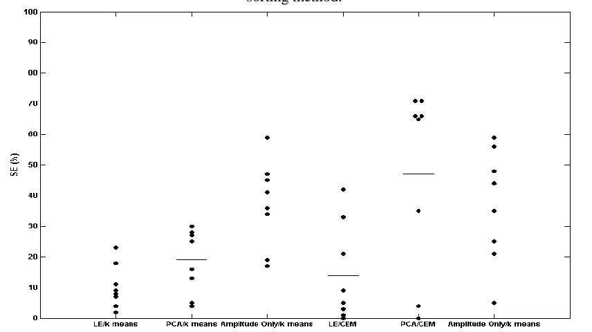
Figure 3. Dot plot of the sorting error results obtained using the spike sorting methods. Each dot represents the sorting error of a single simulated data set using the corresponding spike sorting
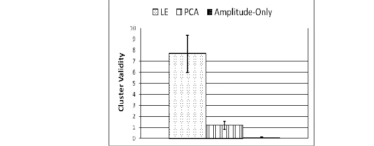
[image:8.612.94.522.403.643.2]To further test the effectiveness of LE feature extraction. The ratio between between-cluster and within-cluster distance (cluster validity) was compared to other features extraction methods employed in this study (Figure 4). Similarly Ganbari et al [27] have tested this ratio their results showed that LE clusters were better separated than PCA clusters.
K 1
i A N
2 i t
2 j i K 1 i j K 2 1 i
i A cc
N 1
CC CC Validity
Cluster
,...., , ,..., ,
min
(12)
[image:9.612.97.467.299.444.2]Where CCi is the centre of cluster of spikes produced by neuron Ni, Nt is the total number of spikes, K is the number of neurons simulated in the recording, and A is the feature vector. This cluster validity represents the ratio between the between-cluster and within-cluster distance. Higher cluster validity indicates better separation. As shown in Figure 4 the mean cluster validity is higher for LE features compared to the other features employed in the study. The differences in cluster validity between all methods are statistically significant (p < 0.0001) as indicated by the Friedman test.
Figure 4. Comparison of mean cluster validity index for the feature extraction methods, Vertical lines indicate standard error
(a) (b)
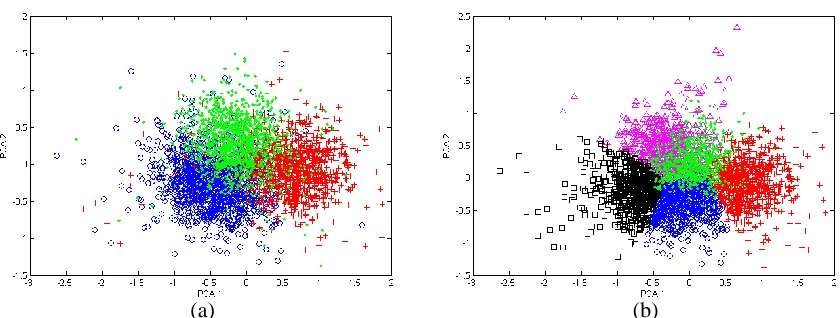
Figure 5. PCA Feature space plots for data set C. Where PCA1 and PCA 2 refers to the first and second principal component respectively (a) PCA feature space of the spikes. (b) PCA feature extraction combined with k-means clustering algorithm output where the PBM index has detected
five clusters.
[image:10.612.95.521.256.455.2](a) (b)
Figure 6. Laplacian eigenmaps feature space plots for data set C. Where LE1 and LE2 refer to the first and second eigenvectors ( f1 and f2 ) respectively (a) LE feature space of the spikes. (b) LE feature extraction combined with k-means clustering algorithm output where the PBM index
has detected four clusters.
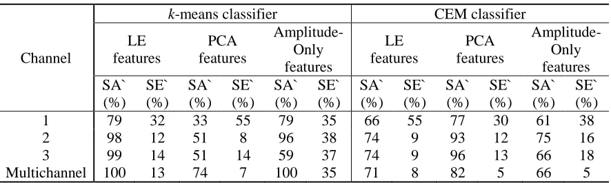
5.3. Spike sorting results using in-vivo recordings:
Table 2. in-vivo data set results.
Channel
k-means classifier CEM classifier
LE features
PCA features
Amplitude-Only features
LE features
PCA features
Amplitude- Only features SA`
(%) SE` (%)
SA` (%)
SE` (%)
SA` (%)
SE` (%)
SA` (%)
SE` (%)
SA` (%)
SE` (%)
SA` (%)
SE` (%)
1 79 32 33 55 79 35 66 55 77 30 61 38
2 98 12 51 8 96 38 74 9 93 12 75 16
3 99 14 51 14 59 37 74 9 96 13 66 18
Multichannel 100 13 74 7 100 35 71 8 82 5 66 5
SA` and SE` refers to the Sorting Accuracy and Sorting Error when the spike sorting algorithm was compared to the experts sorting. The results in Table 2 illustrate that the combination of LE features and k-means clustering yields best sorting performance. In the combination case most methods yield improved performance this illustrates the advantages of tetrode recording. All the spike sorting algorithms performed relatively poorly while sorting the spikes in the first channel, this is attributed to the low amplitude of the spikes in this channel.
6. Discussion
Recently it was reported that Laplacian eigenmaps can aid graphical manual spike sorting [27, 28]. In this paper we extended these findings and propose a fully automated spike sorting algorithm based on LE feature extraction. The results in Table 1 illustrate that there is significant improvement between LE sorting algorithms compared to other automatic sorting algorithms proposed in the literature.
It can be concluded from the results in Table 1 that LE provides the best performance in spike sorting when used alongside k-means clustering. LE combined with CEM also yields good results in spike sorting. Table 2 shows the results obtained using in-vivo recordings confirming the robustness of LE algorithms. However, the performance difference between CEM and k-means algorithms is profoundly more evident when used with LE features. This is primarily due to over-clustering caused by CEM. The CEM algorithms implemented in KlustaKwik assume a Gaussian distribution for the features however the LE features do not follow Gaussian distribution. This could explain the ineffectiveness of LE/CEM combination.
The Amplitude-Only feature set yielded the poorest performance with large sorting error percentages as demonstrated in Table 1. This may be due to electrode drift or complex-spike cells whilst in other cases, the spikes of two neurons may have similar spike amplitude but different widths. The variation in a single neuron amplitude can cause low spike sorting performance. In the case of in-vivo recordings results Table 2, individual channels yield high sorting error percentages or low sorting accuracy. However, when the information from multichannel recording is extracted, the performance of spike sorting using the simple amplitude features increases, thus illustrating the importance of multichannel recording in spike sorting.
channels. Using the PCA and k-means algorithm, merging clusters can increase the sorting accuracy in this case up to ~ 99%.
In some cases, (as shown in Figure 5b), over-clustering occurs. The performance of the spike sorting algorithms can be improved by an additional step that assess the similarity of the spikes in each cluster and merge the cluster of spikes that belong to a single neuron. A human operated method for merging spike clusters based on autocorrelograms and cross-correlograms is proposed in [14]. Over-clustering was encountered in [13] and clusters were merged based on boundary density estimation. Over-clustering is a challenge in spike sorting that has to be addressed. A possible solution to over-clustering is to consider the eigengap heuristic [36], where the ratio between successive eigenvalues can indicate the number of clusters in a data set.
Overlapping spikes is one of the important challenges in automated spikes sorting algorithms. Several methods have been proposed in the literature addressing this problem explicitly. One approach [37] has been cited as computationally expensive, while others have proposed solutions which require less computation power [38]. However these algorithms assume Gaussian noise [39]. Recently, advancement in field has been reported [19, 39-41]. The proposed spike sorting system in this study does not explicitly deal with overlapping spikes. Algorithms that will resolve overlapping spikes in addition to current method proposed in this study may lead to improved performance of the spike sorting system.
7. Conclusion
In this study, an automatic spike sorting method is proposed which is capable of spike detection, identifying the number of neurons recorded and assigning each spike to the neuron that produced it. This method yields significantly improved performance compared to previously reported methods. The method has the limitation of over-clustering in certain cases. In future studies unsupervised clustering methods will be considered to address this issue.
Acknowledgements
This study employed a modified version of the analysis software FIND [42].
References
[1] Kandel E, Schwartz J H, Jessell T. Principles of Neural Science: McGraw-Hill Medical; 2000.
[2] Mitra P P, Bokil H. Observed brain dynamics. New York: Oxford University Press; 2009. [3] Brown E N, Kass R E, Mitra P P. Multiple neural spike train data analysis: state-of-the-art and future challenges. Nat Neurosci. 2004 May;7(5):456-61.
[4] Rizk M, Bossetti C A, Jochum T A, Callender S H, Nicolelis M A, Turner D A, et al. A fully implantable 96-channel neural data acquisition system. J Neural Eng. 2009 Apr;6(2):026002.
[5] Csicsvari J, Henze D A, Jamieson B, Harris K D, Sirota A, Bartho P, et al. Massively parallel recording of unit and local field potentials with silicon-based electrodes. J Neurophysiol. 2003 Aug;90(2):1314-23.
[6] Fee M S, Mitra P P, Kleinfeld D. Variability of extracellular spike waveforms of cortical neurons. J Neurophysiol. 1996 Dec;76(6):3823-33.
[7] Buzsaki G. Large-scale recording of neuronal ensembles. Nat Neurosci. 2004 May;7(5):446-51.
[8] Lewicki M S. A review of methods for spike sorting: the detection and classification of neural action potentials. Network. 1998 Nov;9(4):R53-78.
[10] Takekawa T, Isomura Y, Fukai T. Accurate spike sorting for multi-unit recordings. Eur J Neurosci. 2010 Jan;31(2):263-72.
[11] Franke F, Natora M, Boucsein C, Munk M H, Obermayer K. An online spike detection and spike classification algorithm capable of instantaneous resolution of overlapping spikes. J Comput Neurosci. 2009 Jun 5.
[12] Mukhopadhyay S, Ray G C. A new interpretation of nonlinear energy operator and its efficacy in spike detection. IEEE Trans Biomed Eng. 1998 Feb;45(2):180-7.
[13] Yang Z, Zhao Q, Liu W. Improving spike separation using waveform derivatives. J Neural Eng. 2009 Aug;6(4):046006.
[14] Harris K D, Henze D A, Csicsvari J, Hirase H, Buzsaki G. Accuracy of tetrode spike separation as determined by simultaneous intracellular and extracellular measurements. J Neurophysiol. 2000 Jul;84(1):401-14.
[15] Thakur P H, Lu H, Hsiao S S, Johnson K O. Automated optimal detection and classification of neural action potentials in extra-cellular recordings. J Neurosci Methods. 2007 May 15;162(1-2):364-76.
[16] Abeles M, Goldstein M H, Jr. Multispike train analysis. Proceedings of the IEEE. 1977;65(5):762-73.
[17] Vargas-Irwin C, Donoghue J P. Automated spike sorting using density grid contour clustering and subtractive waveform decomposition. J Neurosci Methods. 2007 Aug 15;164(1):1-18.
[18] Cheeseman P, Stutz J. Bayesian classification (AutoClass): theory and results. Advances in knowledge discovery and data mining: American Association for Artificial Intelligence; 1996. p. 153-80.
[19] Hulata E, Segev R, Ben-Jacob E. A method for spike sorting and detection based on wavelet packets and Shannon's mutual information. J Neurosci Methods. 2002 May 30;117(1):1-12.
[20] Takahashi S, Anzai Y, Sakurai Y. A new approach to spike sorting for multi-neuronal activities recorded with a tetrode--how ICA can be practical. Neurosci Res. 2003 Jul;46(3):265-72.
[21] Harris K D. Available from: http://klustakwik.sourceforge.net/.
[22] Gray C M, Maldonado P E, Wilson M, McNaughton B. Tetrodes markedly improve the reliability and yield of multiple single-unit isolation from multi-unit recordings in cat striate cortex. J Neurosci Methods. 1995 Dec;63(1-2):43-54.
[23] Henze D A, Borhegyi Z, Csicsvari J, Mamiya A, Harris K D, Buzsaki G. Intracellular features predicted by extracellular recordings in the hippocampus in vivo. J Neurophysiol. 2000 Jul;84(1):390-400.
[24] Anderson M I, O'Mara S M. Analysis of recordings of single-unit firing and population activity in the dorsal subiculum of unrestrained, freely moving rats. J Neurophysiol. 2003 Aug;90(2):655-65.
[25] Belkin M, Niyogi P. Laplacian Eigenmaps for Dimensionality Reduction and Data Representation. Neural Computation. 2003;15(6):1373-96.
[26] Chen C, Zhang L, Bu J, Wang C, Chen W. Constrained Laplacian Eigenmap for dimensionality reduction. Neurocomputing. 2010;73(4-6):951-8.
[27] Ghanbari Y, Spence L, Papamichalis P. A graph-Laplacian-based feature extraction algorithm for neural spike sorting. Conf Proc IEEE Eng Med Biol Soc. 2009;2009:3142-5. [28] Ghanbari Y, Papamichalis P, Spence L. Graph-Spectrum-Based Neural Spike Features for Stereotrodes and Tetrodes. IEEE International Conference on Acoustics, Speech, and Signal Processing. 2010:598-601.
[30] Moffitt M A, McIntyre C C. Model-based analysis of cortical recording with silicon microelectrodes. Clin Neurophysiol. 2005 Sep;116(9):2240-50.
[31] Theodoridis S, Koutroumbas K. Pattern recognition. San Diego,: Academic Press; 1998. [32] Pakhira M K, Bandyopadhyay S, Maulik U. Validity index for crisp and fuzzy clusters. Pattern Recognition. 2004;37(3):487-501.
[33] Celeux G, Govaert G. A classification EM algorithm for clustering and two stochastic versions. Computational Statistics & Data Analysis. 1992;14(3):315-32.
[34] Friedman M. The Use of Ranks to Avoid the Assumption of Normality Implicit in the Analysis of Variance. Journal of the American Statistical Association. 1937;32(200):675-701. [35] Sheldon M R, Fillyaw M J, Thompson W D. The use and interpretation of the Friedman test in the analysis of ordinal-scale data in repeated measures designs. Physiother Res Int. 1996;1(4):221-8.
[36] von Luxburg U. A tutorial on spectral clustering. Statistics and Computing. [10.1007/s11222-007-9033-z]. 2007;17(4):395-416.
[37] Atiya A F. Recognition of multiunit neural signals. IEEE Trans Biomed Eng. 1992 Jul;39(7):723-9.
[38] Lewicki M S. Bayesian Modeling and Classification of Neural Signals. Neural Computation. 1994;6(5):1005-30.
[39] Segev R, Goodhouse J, Puchalla J, Berry M J, 2nd. Recording spikes from a large fraction of the ganglion cells in a retinal patch. Nat Neurosci. 2004 Oct;7(10):1154-61.
[40] Zhang P M, Wu J Y, Zhou Y, Liang P J, Yuan J Q. Spike sorting based on automatic template reconstruction with a partial solution to the overlapping problem. J Neurosci Methods. 2004 May 30;135(1-2):55-65.