To Appear in the International Journal for Production Research
Case-Based Reasoning in Scheduling:
Reusing Solution Components
Pádraig Cunningham Department of Computer Science
Trinity College Dublin College Green, Dublin 2
Ireland
[email protected] Tel.: +353-1-6081765 Fax: +353-1-6772204
Barry Smyth
Department of Computer Science University College Dublin
Belfield, Dublin 2 Ireland [email protected]
Abstract
Case-Based Reasoning in Scheduling:
Reusing Solution Components
1 Introduction
There is a lot of optimism at the moment about the usefulness of case-based reasoning (CBR) in the development of knowledge based systems. The view is that cases can represent good quality solutions that may be reused in new situations. Typically, cases represent compiled knowledge in weak theory domains (CAPLAN/CBC as described in (Muñoz, Paulokat & Wess, 1994) is a typical example of this idea.). There are other situations where solution reuse may be advantageous; for instance in optimisation problems where cases can represent highly optimised structures in the problem space. In this paper we explore this type of reuse in job scheduling problems.
Two distinct approaches to case-based scheduling can be identified from the literature. The first one is used in Koton's SMARTplan (1989). Cases are used to propose preliminary schedules which are then adapted (refined and repaired) to satisfy the target schedule requirements. The second approach does not uses cases to propose schedules, but instead to adapt schedules proposed by other methods (for example, Sycara & Miyashita, 1994). In other words cases can encode actual schedules (the first approach) or they can encode repair procedures (the second approach).
In this work we examine the first approach and look at two different modes of reuse -- (1) the reuse of single cases as skeletal solutions, and (2) the reuse of multiple cases as the building blocks of the desired target solution.
In order to explain the manner in which schedule components can be reused we start with an example of the use of CBR in a standard Travelling Salesman Problem. The Euclidean nature of this problem allows the manner in which schedules are reused to be seen graphically.
The core scheduling problem considered here is a single machine problem where job setup time is sequence dependent. We consider two CBR solutions to this problem and we compare these with two standard solution techniques. The first is Simulated Annealing; this produces good quality solutions but is computationally expensive. The second is a naïve search mechanism that selects the nearest job next. This is referred to as the Myopic solution; it produces poorer solutions but is fast.
An extensive evaluation comparing these techniques is presented. Our conclusion is that the CBR techniques produce fairly good quality solutions quickly. The details of the scheduling problem are presented in the next section before the CBR solutions are introduced in section 3. The case retrieval mechanisms are described is section 4 and the evaluation is presented in section 5.
2 Case-Based Reasoning
The basic motivation behind Case-Based Reasoning is that, in many tasks, expert competence may rely heavily on reusing solutions to previously solved problems. The exploitation of this idea in knowledge-based systems (KBS) development produces systems where expertise is encoded implicitly in cases rather than explicitly in rules or models of the problem domain. Evidently this approach to KBS development has important knowledge engineering advantages because the important interactions in the problem domain do not have to be modelled explicitly. Thus CBR is particularly useful in weak theory domains (i.e. problem domains where the important causal interactions are not well understood).
Thus, in the context of all that has been written about the knowledge engineering bottleneck, CBR looks like a ‘free lunch’. It seems to allow for the design of knowledge-based systems without knowledge engineering. Experienced CBR practitioners realise that this in not really the case. In order for a CBR system to work effectively important domain knowledge needs to be encoded in the case indexing structure, in the retrieval mechanism and in case adaptation (Richter ’95).
the features must be predictive of the important characteristics of the problem. A substantial knowledge engineering effort may be required to discover a good set of features. The CBR system must have a retrieval mechanism that can efficiently discover cases similar to the target problem in the case-base. There are many techniques in use but the two most common are based on decision trees or k-nearest neighbour techniques.
Spec
Soln
?
T1
Matching
Engine
Target
Case Base
Spec
Soln
B125
Spec
Soln
B127
Spec
Soln
B125
Spec [image:3.595.136.465.136.514.2]Soln
B103
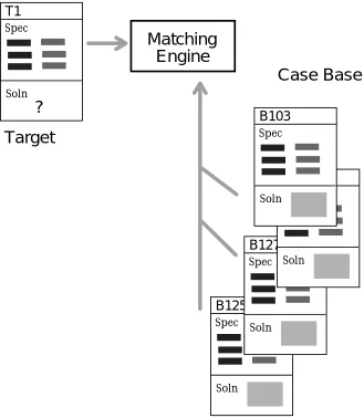
Figure 1. A general model of retrieval in case-based reasoning
Often the most problematic aspect of a CBR system will be the adaptation phase. If the target case is different from the retrieved case it will be necessary to adapt the retrieved solution to account for these differences. The complexity of this adaptation will depend on the complexity of the case solution. In diagnosis and classification tasks the solution is often atomic (i.e. a simple symbol or value) and no adaptation may be required. Whereas in design a solution may have a complex structure and adaptation will have to manipulate this. So the structure and complexity of solutions is an important characteristic in classifying CBR systems because it has strong implications for the amount of adaptation required (Hanney, Keane, Smyth & Cunningham 1995).
Another defining characteristic of CBR systems is the number of cases used to compose a new solution. The standard approach is to use a single case in solving a new problem. However, there has been considerable work on CBR systems that may reuse several cases in solving a new problem. This reuse of several cases may involve combining several cases in a hierarchical solution (Smyth & Cunningham 1992) or several cases may be aggregated in finding a new solution (Redmond, 1990). In this paper we explore a CBR solution to the scheduling problem based on the reuse of a single case and a solution where components of several cases are combined in forming a solution.
its case-base that it has solved itself because learning these cases will not improve the competence of the system. It may improve the performance of the system but ‘speed-up’ learning is not often a strong motivation. This argument suggests that incorporating learning into a CBR system only makes sense where the cases being learned were solved by another agent. This other agent may be an expert user or it may be a software component such as a first-principles planner.
3 The Scheduling Problem
The scheduling problem addressed here involves scheduling N jobs on a single machine in a situation where job setup time is sequence dependent. The manifestation of this problem with which we are concerned arises in electronics assembly where the job setup time on component sequencing machines used in printed circuit board assembly is schedule dependent. The setup time associated with scheduling job B after job A depends directly on the number of components required in B that were not used in A (see Cunningham & Browne, 1987 for more details).
This is an example of a non Euclidean TSP in that solutions cannot be graphed in 2-dimensional space. This scheduling problem is also asymmetric in that the 'distance' from A to B is probably not equal to the 'distance' from B to A. The context of this scheduling problem motivates a case based solution. Typically schedules will be produced on a weekly or monthly basis and the set of jobs to be scheduled may be similar to a set scheduled in the past.
Before presenting our solution to this scheduling problem we will describe T-CBR a case-based solution to a standard TSP that can be described graphically. This will offer some insight into how the reuse of components actually works. We also present an analysis of the case-base size required to offer good coverage in a given domain.
3.1 CBR Solution to a Euclidean TSP
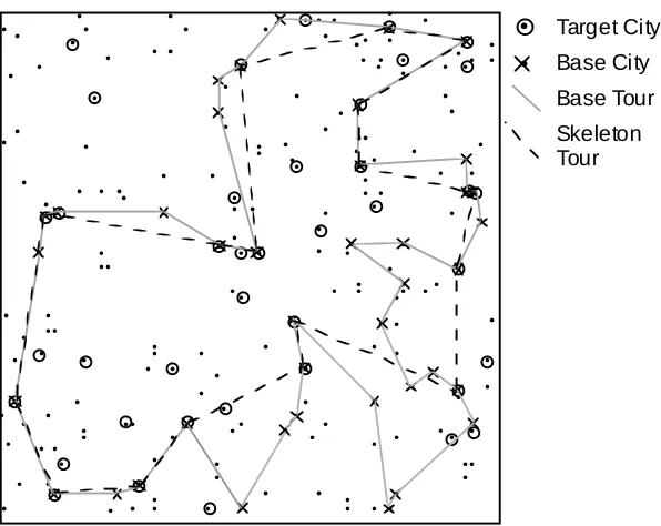
In Figure 2 we show a 'world' of 100 cities, an optimised tour of 40 cities and a target problem of 40 cities. There is an overlap of 19 cities between the base and the target. In T-CBR the size and distribution of this overlap is the measure of similarity used in case retrieval. The first step in the adaptation process is to produce a skeleton tour from the overlap of the base and target; this is shown in the Figure. The first CBR solution is produced by adding the remaining cities on the target to this tour.
Target City
Base City
[image:4.595.154.452.450.687.2]Base Tour Skeleton Tour
The algorithm for this is as
follows:-function Add-cities(tour, rem-cities) {
if rem-cities {
best-city ← Select-best-city(tour, rem-cities) rem-cities ← Remove-city(best-city, rem-cities tour ← Insert-city(tour, best-city)
Add-cities(tour, rem-cities) }
}
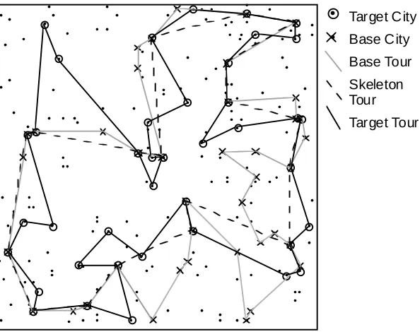
The Select-best-city function takes each remaining city in turn and finds the point on the tour where it can be inserted with the minimum cost. The best city is the one that can be inserted in the tour with least cost. This first CBR solution is shown in Figure 3.
Target City
Base City
Base Tour
Skeleton Tour
[image:5.595.156.453.232.467.2]Target Tour
Figure 3. The first CBR solution for the target shown in Figure 2.
This T-CBR solution is 365 units in length. The SA algorithm produced a solution of 338 units. This T-CBR solution is 8% longer than the SA solution. This adaptation mechanism is inspired by the geometric techniques for solving TSPs used by Norback and Love (1976). However it will work for non geometric or non symmetric problems. T-CBR goes on to improve this initial solution by examining each pair of cities in turn and testing to see if reversing the section of path between these two points produces an improved solution. We call this gradient descent 'Freezing' by analogy with what happens in Simulated Annealing.
3.2 An Analysis of Case Coverage
The size of the case-base depends on a number of factors: n, the number of cities; r the tour lengths of cases and target problems; and k the desired overlap between a target problem and a retrieved case. That
is:-For a domain of n cities and a tour size of r, how many cases are required to ensure the presence of at least one case that shares k or more cities with the target?
First of all the total number of possible tours of size r in this domain (of n cities) is given by equation 1.
(1) Total tours = n r
(2) Total tours sharing k cities = r k
• n−r r−k
The total number of tours that share k or more cities is thus given by equation 3.
(3) Total tours sharing k or more cities = r i i= k r
∑
• n−r r−i
For a particular target specification of r cities, the probability of picking a random tour that shares at least k cities with this target is shown in equation 4; this is termed the probability of success and is denoted by S.
(4) S =
r i i =k r
∑
• n−rr−i
n r
Now in a CBR scenario, a case-base of C random cases means that we have essentially C attempts to find a successful tour, a tour that overlaps by at least k cities with the target. We would like the probability of failure (in other words the probability of there not being a suitable case) to be less than some fraction
ε
. So if (1-S)C is the probability of a finding no such case over C trials* then the relationship betweenε
and S isthe simple one shown in equation 5. (5)
(
1 - S)
C < εSo from this we can form the function in equation 6 that computes the case-base size necessary to ensure that a suitable case is present for every target problem, all but ε×100% of the time.
(6) C = log
( )
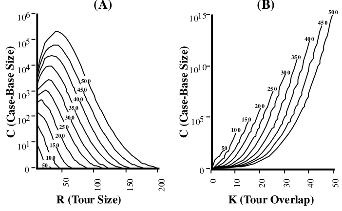
ε log(1 - S)Figure 4 (A) & (B) illustrate how this function behaves for various values of n, r, and k. In each graph, the error value,
ε
, is kept static at 0.05, and n is varied from 50 to 500 in increments of 50, a separate curve is drawn for each n value and marked with that value. Both graphs plot the case-based size on the y axis, which is logarithmically scaled.C
(C
as
e-Bas
e S
iz
e)
0 105 010 20 30 40 50
K (Tour Overlap)
0 101 50 10 0 15 0 20 0
C (
C
a
se
-Bas
e S
iz
e)
R (Tour Size)
1010 1015 102 103 104 105 106
(B)
(A)
50 10 0 15 0 20 0 25 0 30 0 40 0 35 0 50 0 45 0 50 10 0 15 0 20 0 25 0 30 0 35 0 40 0 45 0 50 0Figure 4. Variations in case-base size.
[image:6.595.127.478.467.683.2]
Figure 4(A) plots case-base size against the tour length (that is the case and target sizes). The desired overlap between target and case, k, is assumed to be 30% of the tour length. As expected there are large variations in the size of the case-base as n and r increase. It is interesting that for this 30% overlap restriction, the size of case-base needed for a given n peaks when r is 12.5% of n and trails off rapidly as r increases towards n. For example, for n = 500, the case-base size offering 30% overlap, peaks at r = 40, where over 105 cases are needed to provide the desired problem coverage. However, when the tour size is 100, less than 600 cases are needed.
Figure 4(B) plots the case-base size against varying overlap. For each curve r is fixed at 20% of n and the overlap, k, is varied from between 0 and r/2. So for example, the curve corresponding to n = 500 corresponds to a system where the tour length (that is the sizes of the cases and the target problems) is 100, and a varying overlap of between 0 and 50 cities. Again, as expected the case-base size rises exponentially with k. In a system where n is 500, r is 100, and k is 50 (that is 50% of the tour length), a case-base of over 1014 cases is required. However, as was mentioned above, if an overlap of 30 cities is acceptable for this system then less that 600 cases are needed.
A pessimistic interpretation of these results might suggest that CBR and TSP do not mix well, owing to the enormous case-bases required to provide adequate coverage and significant performance improvements. However this is not necessarily true in general, and there exist a great many TSP problems which are amenable to a case-base solution, at least in the sense that the case-base is of an acceptable size. In particular, this is true if the route size r is greater than roughly 20% of n and k is less that about 40% of r.
4 Two CBR Solutions in Scheduling
The data used in the scheduling experiments describe a hypothetical situation. There is a total of 500 jobs that may need to be scheduled periodically. Each job has between 40 and 80 components taken from a set of 200 components. The cost of scheduling job B after job A is represented by the number of components in B not in A, as said before. There is also a case-base of 600 good quality schedules of 100 jobs each taken from the population of 500 jobs. These schedules were produced using simulated annealing (see Cunningham & Smyth, 1995 for details of the algorithm). *
In this paper we consider two alternative CBR solutions to this scheduling problem. The first solution we call the skeletal solution. This reflects the way in which the best matching case retrieved from the case-base is used to form a skeleton on which the new schedule is built. In this situation only one case from the case base is retrieved; the jobs that this case has in common with the target case make up the skeleton and the remaining cases are added to this skeleton using the algorithm described in section 3.1.
The other CBR approach is radically different in that several cases are used in building a solution to the target problem. We call this the building block solution because sub-sections of the target schedule are discovered in cases in the case-base and composed into a new schedule to satisfy the target problem. The first step in this process is to retrieve these sub-sections of schedule from the case-base (see section 5 for more details). These schedule bits are contiguous sections of existing optimised schedules that contain only jobs on the target schedule.
schedule ← starting job
function Add-bits(schedule, bits-pool) {
if bits-pool{
best-bit ← Select-best-bit(schedule-end, bits-pool)
if Close-to-schedule(best-bit){
schedule ← Concatenate(schedule, best-bit)
bits-pool ← Remove-unusable-bits(schedule, bits-pool)
Add-bits(schedule, bits-pool)
} }
}
The Select-best-bit function tries two things; first it looks for the longest bit that starts at the current
end point of the incomplete schedule (same job), if it fails on this is selects the bit that starts closest to the current end point. Each time the schedule is extended, bits are removed from the pool if they contain jobs that are now already in the schedule. This process produces a schedule that is still missing some jobs; these jobs are added in using the process described in the skeletal solution.
We feel this building block approach is the more important for scheduling in general because it involves reusing fragments of optimised structure in new situations. This strategy has the potential for reuse in more complex scheduling problems.
5 Case Retrieval
Two different approaches to retrieval are described. One works to select a single best skeletal case which is reused as a template for the target solution; some jobs will be dropped from the template, some will be added. The other approach returns a collection of solution sequences, each of which may be used intact to produce a part of the target schedule.
5.1 Case Retrieval for the Skeletal Solution
Selecting a skeletal solution involves searching for a case which satisfies two criteria. First, the case must share a significant portion of the target jobs. Second, these jobs must be distributed as evenly as possible throughout the case solution – concentrations of target jobs do not make good skeletal solutions.
The pseudo-code below describes how the case-base is searched for the best possible skeleton as a two step process. The first step, base filtering, only accepts cases whose overlap with the target case suggests the possibility of a good skeletal solution; if a case intersects with the target in only a few jobs then it is unlikely to yield a suitable skeletal solution.
function Retrieve-Skeleton(target-jobs, case-base) { base-cases ← Base-Filter(target-jobs, case-base) best-case ← First(base-cases)
best-score ← Skeletal-Quality(best-case)
For each base-case in Rest(base-cases) {
base-score ← Skeletal-Quality(target-jobs, base-case)
if base-score > best-score {
best-score ← base-score best-case ← base-case }
The second step chooses a single case by using a metric that measures skeletal solution quality in terms of the number of jobs in the skeletal solution and the evenness of the distribution of these jobs through the entire base solution.
function Skeletal-Quality(target-jobs, base-case) { shared-jobs ← Intersection(target-jobs, base-case) StdDev ← Skeletal-Deviation(shared-jobs, base-case)
qual len base case StdDev len base case len shared jobs
len base case
← − − × − × −
−
[ ( ) ( ))] ( )
( )
2
Return(qual)
}
This "evenness" factor is a measure of the distribution of the target jobs in the base job sequence. The lengths of segments of the base sequence that do not contain target jobs are obtained and the standard deviation of these lengths is calculated. Large deviations are indicative of uneven skeletons and result in poor quality (low values) measures1.
So the function Skeletal-Deviation measures the unevenness of the overlap in a skeletal solution.
function Skeletal-Deviation(shared-jobs, base-case){ position-list ← Positions(shared-job, base-case)
difference-list ← Positional differences between adj. shared-jobs
mean difference
diff
difference list
diff difference list
− ←
−
∈
∑
−deviation
mean difference diff
difference list
diff difference list
←
− −
−
∈
∑
−( )2
Return(deviation) }
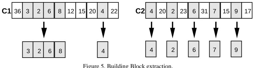
For example, consider the target specification (T) containing 10 jobs {0,1,2,3,4,5,6,7,8,9}. Suppose cases C1 and C2 encode the following schedules, {36,3,2,6,8,12,15,20,4,22} and {4,20,2,23,6,31,7,15,9,17}. Both cases share 5 jobs with the target. However the skeletal deviation of C1 is 1.68 (with a mean difference of 1.75) and for C2 it is 0 (with a mean of 2); the target jobs are evenly distributed through C2 but concentrated in the first half of C1. The result is that the quality of C1's skeleton is 41.6 while C2's is 50. In other words C2 is preferred over C1.
5.2 Case Retrieval for the Building Block Approach
The building block retrieval algorithm uses the same base filtering process as the skeletal retrieval algorithm (although the intersection threshold is generally set to a lower value). The main difference between the procedures is that instead of using a quality metric, building block retrieval calls a function which breaks a case solution up into reusable building block sequences (schedule bits). These bits are collected and those large enough (≥3 jobs) are returned to be used later in composing the final target solution.
function Retrieve-Building-Blocks(target-jobs, case-base) {
bits ← {}
base-cases ← Base-Filter(target-jobs, case-base)
For each base-case in base-cases {
bits ← bits + Extract-Bits(target-jobs, base-case)
}
Return (bits)
}
The first step in the bit extraction procedure (shown below) is to mark the end (and start) positions of each reusable bit by noting the positions of any jobs in the base case that are not in the target. The base solution sequences between these positions are reusable as building blocks because they contain only target jobs. If such a block contains 3 or more jobs then it is returned by the Extract-Bits function.
function Extract-Bits(target-jobs, base-case){ bits ← {}
unwanted-jobs ← Set-Difference(base-case, target-jobs) bit-ends ← Positions(unwanted-jobs, base-case)
bit-start ← First(bit-ends)
For each bit-end in Rest(bit-ends) {
bits ← bits + Extract-Bit(base-case, bit-start, bit-end) bit-start ← bit-end
}
Return(Bits)
}
Figure 5 shows how reusable bits are extracted from C1 and C2 (the cases of the previous example) according to the jobs specified in the target sequence T. The unshaded jobs represent the edges of reusable bits and the shaded sections (which contain only target jobs) can be extracted for potential reuse. The interesting thing to note is that C1 is far more useful than C2 when the building block approach is used; this is in complete contrast to the skeletal approach where C2 was deemed to be more useful. In fact in this example C2 yields no useful bits (> 2 jobs in length) where as C1 yields a 4-job bit.
36 3 2 6 8 12 15 20 4 22
C1
3 2 6 8 4
4 20 2 23 6 31 7 15 9 17
C2
[image:10.595.98.510.427.538.2]4 2 6 7 9
Figure 5. Building Block extraction.
S iz e
Av
g
.
Nu
mb
e
r
0 2 0 4 0 6 0 8 0 1 00 1 20 1 40 1 60 1 80 2 00
3 4 5 6 7 8
0 .12 0 .28
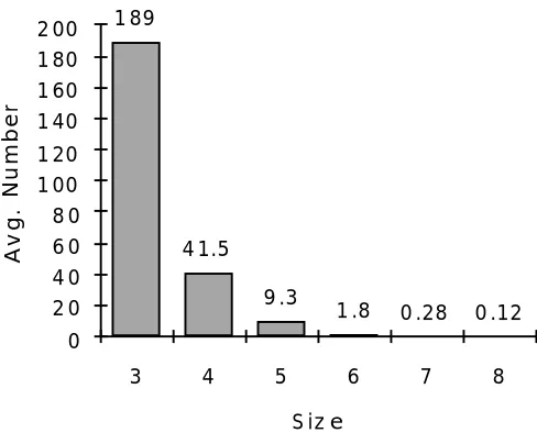
[image:11.595.184.428.73.270.2]1 .8 9 .3 4 1.5 1 89
Figure 6. Average numbers of blocks retrieved for the Building Block solution
6 System Evaluation
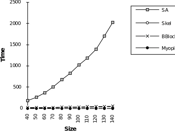
Two issues are addressed in the evaluation process. We compare the solution quality and solution time of the two CBR techniques with the two alternatives mentioned already. We also evaluate how these techniques perform as the size of the target problem is increased. This second evaluation is particularly relevant because the time taken by the annealing technique increases more than linearly with the problem size.
6.1 Solution Quality & Time
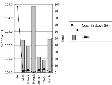
We have said already that medium quality solutions to TSPs can be improved by the “Freezing” technique described in section 3.1. This measure does not produce any significant improvement in the SA solution; however it does improve the other three. Thus in evaluating solution time and quality we consider seven alternatives in total.
As mentioned already, the case-base in use in this evaluation contains 600 good quality schedules produced using SA. This size of case-base is chosen so that a case overlapping a target problem by 30% can expect to be retrieved. Figure 7 shows data drawn from running the seven solution techniques on 100 different target problems. The average times and average schedule lengths were calculated. The key point here is that the SA takes about 30 times longer than the CBR alternatives.* It can be seen from the graph that, compared with the time taken for the SA, there is little to choose between the CBR techniques. In turn, the Myopic solution time is negligible compared to these.
100.0 101.0 102.0 103.0 104.0 105.0
SA
Skel
BBlock Myopic Skel+Fr BB+Fr My+Fr
% above SA
0 10 20 30 40 50 60 70 80 90 100
Time
Cost (% above SA)
[image:12.595.99.476.77.363.2]Time
Figure 7. An evaluation of the solution time and solution quality of the different algorithms.
The solution quality is plotted as a percentage above the average solution obtained with SA. The CBR solutions are within 2% to 2.3% of the SA solution with the Building Block with Freezing solution improving to within 1% of SA. The Myopic solution is 5% above the best value and improves to 2.5% with freezing. So the BB+Freezing solution emerges as a source of good quality solutions in a fraction of the time taken by SA.
6.2 Variations in schedule size
It is clear from an examination of the workings of the CBR techniques that they can be used to produce solutions for problems of a size different to those in the case-base. In this part of the evaluation we consider target problems varying in size from 40 to 140 in steps of 10; 20 problems are analysed at each step. It can be seen in Figure 8 that the skeletal solution quality remains more or less constant at around 2.5% above the SA values. The building block solutions appear to degrade slightly with problem size.
S iz e
% a
b
ov
e
S
A
0 1 2 3 4 5 6
40 50 60 70 80 90
10
0
11
0
12
0
13
0
14
0
S kel
[image:13.595.189.416.71.301.2]BB lock Myopic
Figure 8. Variations in solution quality with target problem size.
There is one final caveat however. The time it takes the simulated annealing technique to find a schedule can be controlled by altering the annealing schedule so we can adjust the solution time for SA down to that of the CBR techniques. Evidently this will result in a deterioration in the solution quality. However, when we tried this we found that fast SA (i.e. same execution time as TSP technique) produced solutions that were only ½% worse than those produced using the building blocks solution described above. So while we have shown that CBR can be used in scheduling, in situations where SA can be used to produce solutions, it should still be considered.
Size
T
im
e
0 500 1000 1500 2000 2500
40 50 60 70 80 90
10
0
11
0
12
0
13
0
14
0
SA
Skel
BBlock
Myopic
Figure 9. Variations in solution time with target problem size.
7 Conclusions & Future Work
[image:13.595.156.447.420.640.2]and a building block approach where several solutions are merged. We argue that this building block approach will be usable in other more complex scheduling problems.
There are two caveats however. It appears that schedule adaptation will be highly problem dependent. In new scheduling scenarios the success of these reuse-based techniques will depend on discovering good adaptation methods. Case retrieval time will probably increase linearly with case-base size. This will be an issue where large case-bases are required to give good coverage.
Our next step is to evaluate this building block technique on more complex scheduling problems.
References
CUNNINGHAM P., SMYTH B., 1995, On the use of CBR in optimisation problems such as the TSP, Case-Based Reasoning Research and Development, Lecture Notes in Artificial Intelligence, edited by M. Veloso & A. Aamodt, (Springer Verlag), pp401-410.
CUNNINGHAM P., BROWNE J., 1986, A LISP-based heuristic scheduler for automatic insertion in electronics assembly, International Journal of Production Research, 24, 1395-1408.
GOLDBERG D.E., 1989, Genetic Algorithms in Search Optimization & Machine Learning, (Reading, MA: Addison Wesley).
HANNEY K., KEANE M., SMITH B. & CUNNINGHAM P., 1995, Systems, tasks and adaptation knowledge: Revealing some revealing dependencies, Case-Based Reasoning Research and Development, Lecture Notes in Artificial Intelligence, edited by M. Veloso & A. Aamodt, (Springer Verlag), pp461-470.
KIRKPATRICK S., GELATT C.D., VECCHI M.P., 1983, Optimization by Simulated Annealing, Science, 220, 671-680.
KOTON, P.,1989, SMARTplan: A Case-Based Resource Allocation and Scheduling System. Proceedings of the Case-Based Reasoning Workshop, 285-289, (Morgan Kaufmann).
MUÑOZ H., PAULOKAT J., WESS S., 1994, Controlling Nonlinear Hierarchical Planning by Case Replay, Advances in Case-Based Reasoning, Lecture Notes in Artificial Intelligence, edited by Haton J-P., Keane M., and Manago M., (Springer Verlag), pp266-279.
NORBACK J., LOVE R., 1977, Geometric Approaches to Solving the Travelling Salesman Problem, Management Science, July 1977, pp1208-1223.
REDMOND, M. A., 1990, Distributed Cases for Case-Based Reasoning: Facilitating the Use of Multiple Cases. Proceedings of AAAI-90, (AAAI Press/ MIT Press), 304 - 309.
RICHTER M., 1995, On the notion of similarity in case-based reasoning, Mathematical and Statistical Methods in Artificial Intelligence, edited by G. della Riccia et al., (Springer Verlag), pp171-184. SMYTH B., CUNNINGHAM P., 1992, Déjà Vu: A Hierarchical Case-Based Reasoning System for Software
Design, in Proceedings of European Conference on Artificial Intelligence, edited by Bernd Neumann, (John Wiley), pp587-589.