Online Full Text

Abstract— The medical diagnosis of most pathologists requires the analysis of the image studies. Therefore, it is important to get the best quality of the images without noise and highlight the details of tissues. The principal aim of this work is to apply different algorithms and filters to reduce the noise of magnetic resonance brain images, due to the noise in these can cause to give a difficult diagnosis. The algorithms considered in this work are the fast mean filter, fast Gaussian filter, and fast median filter; also was used parallel programming in OpenMP. The results show that the parallel implementation of algorithms has more performance in the time processing, localization, and noise reduction than sequential and classic implementation.

Index Terms— MRI brain image, fast mean filter, fast median

filter, fast gaussian 2D, parallel programming, OpenMP.

I. INTRODUCTION

EDICAL imaging is the technique and process used to create images anatomic, physiological or functional of the human body for clinical purposes or medical purpose. There are many different medical image modalities like CT, PET, MRI, X-ray, Ultrasound imaging, etc.

These modalities have different features and are used as pre requirements. Due the size of each image is very large; analyze these modalities takes much time to process sequentially. So, if we divide this sequential processing to efficient parallel processing then we can find good results in a very reasonable time or if we are able to process basic steps like image enhancement, morphological operation, feature calculation quickly then it will be beneficial for medical practice. Hence, by using parallel computing we can save time and money and we can solve large problems in very

Manuscript received July 02, 2019. This work was supported by Vicerrectorado de Investigación, Universidad Técnica Particular de Loja UTPL, Av. Marcelino Champagñat s/n, Loja Ecuador.

L. Cadena, is with Electric and Electronic Department at Universidad de las Fuerzas Armadas ESPE, Av. Gral Ruminahui s/n, Sangolqui Ecuador. (phone: +593997221212; e-mail: [email protected]).

D. Castillo is with the Chemistry and Exact Sciences Department, Universidad Técnica Particular de Loja UTPL, Av. Marcelino Champagñat s/n, Loja Ecuador (e-mail: [email protected]) and also with I3M, Universitat Politècnica de Valencia, Camino de Vera, 46022 Valencia-Spain.

A. Zotin is with Department of Informatics and Computer Techniques, Reshetnev Siberian State University of Science and Technology, 31 krasnoyarsky rabochу av., Krasnoyarsk 660037, Russian Federation (e-mail: [email protected]).

F. Cadena is with College Unidad Educativa Atahualpa. Oyacoto-Quito, Ecuador (e-mail: [email protected])

G. Cadena is with Medicine Faculty at Universidad Central del Ecuador, Iquique 132, Quito-Ecuador (e-mail: [email protected])

P. Diaz Guzman is with Health and Medical Science Department at Universidad Técnica Particular de Loja UTPL, Av. Marcelino Champagñat s/n, Loja Ecuador. (e-mail: [email protected])

Y. Jimenez is with the Chemistry and Exact Sciences Department, Universidad Técnica Particular de Loja UTPL, Av. Marcelino Champagñat s/n, Loja Ecuador (e-mail: [email protected]).

short time periods. Parallel computing provides concurrency and by this we can use non-local recourses very efficiently. It also removes the limit of serial computing.

Medical image processing has experienced dramatic expansion and has been an interdisciplinary research field attracting expertise from applied mathematics, computer sciences, engineering, statistics, physics, biology and medicine. Computer-aided diagnostic processing has already become an important part of clinical routine. Accompanied by the rush of new development of high technology and use of various imaging modalities, more challenges arise; for example, how to process and analyze a significant volume of images so that high quality information can be produced for disease diagnoses and treatment.

One of the recent innovations in computer engineering has been the development of multicore processors, which are composed of two or more independent cores in a single physical package. Today, many processors, including digital signal processor (DSP), mobile, graphics, and general-purpose central processing units (CPUs) have a multicore design, driven by the demand of higher performance. Major CPU vendors have changed their strategy away from increasing the raw clock rate to adding on-chip support for multi-threading by increasing the number of cores; dual- and quad-core processors are now commonplace. Signal and image processing programmers can benefit dramatically from these advances in hardware by modifying single-threaded code to exploit parallelism to run on multiple cores.

This work present medical images processing of MRI with the principal aim to show a simple and efficient technique to remove noise from the medical images, which combines median filtering, mean filtering and Gauss filter to determine the pixel value in the noise less image.

Magnetic resonance imaging (MRI) has created a lot of interest between Medical Professionals and patients, because it provides anatomical and physiological information in a non-invasive way. MRI does not use any kind of ionizing radiation. MRI creates images of structures through the interactions of magnetic fields and radio waves with tissues. Knowledge of the probable pathology is fundamental, choosing the appropriate technique and analyzing the correct region of the body.

Further, MRI is an imaging technique that produces high quality images of the anatomical structures of the human body, especially in the brain, and provides rich information for clinical diagnosis and biomedical research [9,10]. It is the most commonly used imaging modality as it offers high-resolution images in a noninvasive and safe method, without exposing patients to ionizing radiation. Significant attention is given also to two applications for which MRI has unique

Processing MRI Brain Image using OpenMP

and Fast Filters for Noise Reduction

Luis Cadena, Darwin Castillo, Aleksandr Zotin, Patricia Diaz, Franklin Cadena, Gustavo Cadena,

Yuliana Jimenez

potential: blood flow imaging and quantification, and functional neuroimaging based on exploiting dynamic changes in the magnetic susceptibility.

Additionally, MRI technique has become a critically important tool in diagnosis and differentiation of different demyelinating disorders, because it offers high-resolution images in a noninvasive and safe method, without exposing patients to ionizing radiation. Thus, MRI uses magnetic field gradients to modify the frequency and phase of the MR signal in a controlled manner. The images are reconstructed through mathematical algorithms to convert the collected MR signals into spatial information [1-12].

II. DIGITAL PROCESSING OF IMAGES

The digital processing of images consists of algorithmic processes that transform an image into another in which certain information of interest is highlighted, and/or the information that is irrelevant to the application is attenuated or eliminated. For remove noise we used fast filters, and to evaluate quality used SSIM measure. Following we describe these methods.

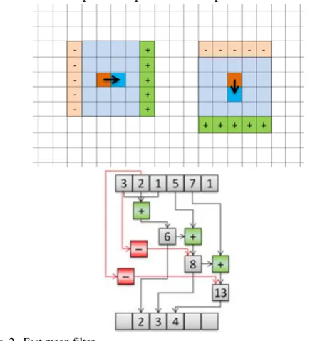
Classic and fast mean filter

The arithmetic classic mean filter is defined as the mean of all pixels spectrum within a local region of an image.

Fig. 1. Classic mean filter.

The fast mean filter obtained by accumulation of the neighborhood of pixel P(y,x), shares a lot of pixels in common with the accumulation for pixel P(y,x+1). This means that there is no need to compute the whole kernel for all pixels except only the first pixel in each row. Successive pixel filter response values can be obtained with just add and a subtract to the previous pixel filter response value.

Fig. 2. Fast mean filter.

Classic and fast median filter

Classic median filter replaces the value of a pixel spectrum by the median of the spectrum levels in the neighborhood of that pixel.

Median filtering is a commonly applied non-linear filtering technique that is particularly useful in removing speckle and salt and pepper noise. It works by moving through the image pixel by pixel, and replacing each value with the median

Fig. 3. Classic median filter.

value of neighbor pixels.

The fast median filter is obtained through the histogram of spectrum for median calculation can be far more efficient because it is simple to update the histogram from window to window. Thus the histogram used for accumulating pixels in the kernel and only a part of it is modified when moving from one pixel to another [8-13, 16].

Fig. 4. Fast median filter.

Classic and fast 2D Gauss filter

Gauss 2D classic filter calculate kernel Gauss bell G(x,y), take pixels from gray value image A in kernel area and add to sum considering Gaussian coefficient, and put obtained value in study pixel in image B.

The Gaussian filter uses a Gaussian function (which also expresses the normal distribution in statistics) for calculating the transformation to apply to each pixel in the image.

The equation of a Gaussian function in one dimension is

2 2

2

2 1 )

( 

 

x

e x

G



 

In two dimensions, it is the product of two such Gaussians, one in each dimension:

2 2 2

2 2

2 1 ) ,

( 

 

y x

e y

x G

   

where x is the distance from the origin in the horizontal axis, y is the distance from the origin in the vertical axis, and σ is the standard deviation of the Gaussian distribution.

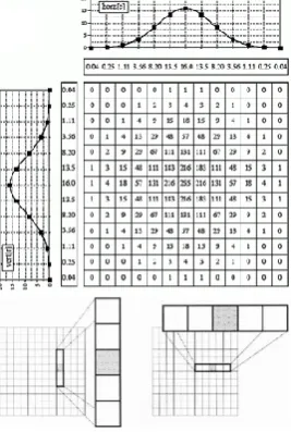
about three standard deviations from the mean. Thus it is possible to truncate the kernel size at this point. Sometimes kernel size truncated even more. Thus after computation of Gaussian Kernel, the coefficients must be corrected that way that the sum of all coefficients equals 1. Once a suitable kernel has been calculated, then the Gaussian smoothing can be performed using standard convolution methods. The convolution can in fact be performed fairly quickly since the equation for the 2-D isotropic Gaussian is separable into y and x components. In some cases the approximation of Gaussian filter can be used instead of classic version [13-19].

Fig. 5. Separable 2D Gauss filter.

Parallel programming in OpenMP

Parallel Programming may speed up code. Today computers have one or more CPUs that have multiple processing cores (Multi-core processor). This helps with desktop computing tasks like multitasking (running multiple programs, plus the operating system, simultaneously). For scientific computing, this means the ability in principle of splitting up computations into groups and running each group on its own processor.

Two main paradigms talk about here are shared memory versus distributed memory models. In shared memory models, all multiple processing units have access to the same memory space. This is the case on desktop or laptop with multiple CPU cores. In a distributed memory model, multiple processing units each of their have their own memory store, and information is passed between them. This is the model that a networked cluster of computers operates with. A computer cluster is a collection of standalone computers that are connected to each other over a network, and are used together as a single system.

The methodology in our case of the algorithms (filters) for processing images is:

1.- Select Kernel

2.- Evaluate denoise filter with parallel OpenMP #pragma omp parallel for

for (int y=0; y< Image_Height; y++) for (int x=0; x< Image_Width; x++) {

// do denoise filters }

3.- Processed pixel put in study pixel of image denoise

OpenMP is an API that implements a multi-threaded, shared memory form of parallelism. It uses a set of compiler directives that are incorporated at compile-time to generate a multi-threaded version of program code. OpenMP is designed for multi-processor/core, shared memory machines [20-24].

Measure PSNR and SSIM

Any processing applied to an image may cause an important loss of information or quality. Image quality evaluation methods can be subdivided into objective and subjective methods. Subjective methods are based on human judgment and operate without reference to explicit criteria. Objective methods are based on comparisons using explicit numerical criteria, and several references are possible such as the ground truth or prior knowledge expressed in terms of statistical parameters and tests.

The next equations show the relationship between the SSIM (structural similarity index measure) and the PSNR (peak-signal-to-noise ratio) for grey-level (8 bits) images. Given a reference image f and a test image g, both of size M×N, the PSNR between f and g is defined by:

𝑃𝑆𝑁𝑅(𝑓, 𝑔) = 10𝑙𝑜𝑔10(

2552

𝑀𝑆𝐸(𝑓, 𝑔))

where

𝑀𝑆𝐸(𝑓, 𝑔) = 1

𝑀𝑁∑ ∑(𝑓𝑖𝑗− 𝑔𝑖𝑗)

2 𝑁

𝑗=1 𝑀

𝑖=1

The PSNR value approaches infinity as the MSE approaches zero; this shows that a higher PSNR value provides a higher image quality. At the other end of the scale, a small value of the PSNR implies high numerical differences between images.

The structural similarity (SSIM) index is designed to improve on traditional methods such as peak signal to noise ratio (PSNR) and mean squared error (MSE), which have proven to be inconsistent with human visual perception.

Structural information is the idea that the pixels have strong interdependencies especially when they are spatially close. These dependencies carry important information about the structure of the objects in the visual scene. Luminance masking is a phenomenon whereby image distortions (in this context) tend to be less visible in bright regions, while contrast masking is a phenomenon whereby distortions become less visible where there is significant activity or "texture" in the image.

The mean structural similarity index is computed as follows:

Firstly, the original and distorted images are divided into blocks of size 8 x 8 and then the blocks are converted into vectors. Secondly, two means and two standard derivations and one covariance value are computed from the images as:

𝜇𝑥=

1

𝑇∑ 𝑥𝑖

𝑇

𝑖=1

𝜇𝑦=

1

𝑇∑ 𝑦𝑖

𝑇

𝑖=1

𝜎𝑥2=

1

𝑇 − 1∑(𝑥𝑖− 𝑥̅)

2 𝑇

𝑖=1

𝜎𝑦2=

1

𝑇 − 1∑(𝑦𝑖− 𝑦̅)

2 𝑇

𝜎𝑥𝑦2 =

1

𝑇 − 1∑(𝑥𝑖− 𝑥̅)

𝑇

𝑖=1

(𝑦𝑖− 𝑦̅)

Thirdly, luminance, contrast, and structure comparisons based on statistical values are computed, the structural similarity index measure between images x and y is given by:

𝑆𝑆𝐼𝑀(𝑥, 𝑦) = (2𝜇𝑥𝜇𝑦+ 𝑐1)(2𝜎𝑥𝑦+ 𝑐2) (𝜇𝑥2+ 𝜇𝑦2+ 𝑐1)(𝜎𝑥2+ 𝜎𝑦2+ 𝑐2)

where c1 and c2 are constants [25].

III. EXPERIMENTAL RESULTS

Different images, with different sizes were processed with classic and fast filters: mean, median, Gaussian 2D. For the experiment used PC based on Intel Core i5 3.1 GHz with 8 GB RAM. The results were obtained by measuring the processing time of 80 different images (for each image, 400 measurements were taken). The results are presented in Fig. 6-8 and Tables I-IV.

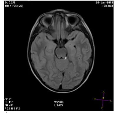
Brief description of medical images used:

MRI Brain: The image presents a calcification between the cortex and the stem. These images are very sensitive for study of congenital and acquired structural anomalies such as infectious, hemorrhagic, tumor, degenerative, and chronic pathologies.

Fig. 6 shows processing time of classic and fast or optimized filters for different image size (4 threads OpenMP). In addition, a study of fast filter implementations was made. It showed the magnitude of the acceleration relative to the sequential implementation of the classical version of the filters. The result of this study was represented as the maps of acceleration of fast filters, showing acceleration coefficient depending on the kernel size (Fig. 6). Also, the acceleration stability of fast algorithms was evaluated depending on the size of the core and the number of threads used. To estimate the acceleration, the mean values obtained during the 300 measurements were taken for each combination of the kernel size and the number of threads.

The experimental results show that the increase in the processing speed for different kernel sizes is almost the same. Some stability is observed in the acceleration for two threads as well as one can see the increase of the acceleration coefficient in the case with more than two threads having the kernel size larger than 5×5. Acceleration with the usage of four threads demonstrates poor efficiency as parts of the CPU resources are spent on background tasks (Fig. 6).

In addition to the speed evaluation, evaluations of noise suppression characteristics were also performed. To simulate the noise which may occur in the equipment, the following noise filter were used. Thus, in the noise filter was layered over the image, the additive noise part was 80%, while the impulse noise part was 20%. The magnitude of additive noise component considered at maximum as 60% of the dynamic range of the experimental data.

The experiments were carried out as follows. For each noise level, 300 noise maps were generated, which were superimposed on the original image. Next, filters (with different kernel sizes) were applied to the noisy image and the PSNR and SSIM metrics were calculated.

a)

b)

c)

Fig. 6. Evaluation of optimized (fast) filters acceleration: (a) Mean filter; (b) Gaussian filter; (c) Median filter.

We conducted experimental research on MRI brain medical images Fig. 7.

Fig. 7 Test image.

TABLE I.

PSNR EVALUATION_OPTIMIZED FILTERS IN dB Noise data Kernel

Size

Filter

Level PSNR Mean Gauss Median

10% 19,4337

3×3 26,4499 26,6162 31,4632 5×5 25,4441 26,3348 26,0941 7×7 24,4246 25,9878 24,0914 9×9 23,9051 25,9163 23,5251 11×11 23,4213 25,9019 23,0034

15% 17,7498

3×3 25,0951 25,2115 31,3586 5×5 24,6368 25,4533 25,7129 7×7 24,0103 25,3044 24,1180 9×9 23,5739 25,2658 23,5490 11×11 23,1413 25,2572 23,0291

20% 16,4937

3×3 23,9026 23,9860 31,0633 5×5 24,0798 24,6117 26,1548 7×7 23,5122 24,5513 24,1792 9×9 23,1564 24,5395 23,6019 11×11 22,7774 24,5358 23,0754

25% 15,6150

3×3 23,0048 23,0674 30,8252 5×5 23,4580 23,8787 26,1362 7×7 23,0348 24,2929 24,2111 9×9 22,7388 24,1965 23,6280 11×11 22,4073 23,8957 23,1053

TABLE II

SSIM VALUES (%) OPTIMIZED FILTERS Noise data Kernel

Size

Filter

Level SSIM Mean Gauss Median

10% 30,8309

3×3 52,5261 52,9341 98,9732 5×5 56,8031 58,4583 96,8460 7×7 55,3762 59,2824 94,6519 9×9 52,2012 59,1818 92,5806 11×11 48,9455 59,1173 90,5115

15% 20,3248

3×3 40,5656 40,9190 98,7282 5×5 45,6737 47,3892 96,3257 7×7 45,0116 48,2220 94,5730 9×9 42,2631 48,1409 92,5113 11×11 39,3629 48,0626 90,4537

20% 14,6082

3×3 32,5422 32,8148 98,1682 5×5 38,5104 39,4721 96,6738 7×7 38,5305 40,8086 94,4997 9×9 36,5191 40,8399 92,4367 11×11 34,1926 40,7849 90,3801

25% 11,4076

3×3 27,5511 27,7515 97,3491 5×5 34,0901 34,7222 96,5549 7×7 34,9439 36,4118 94,4181 9×9 33,5629 36,5819 92,3665 11×11 31,6682 36,5630 90,3168

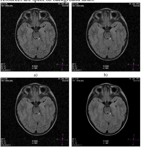
Visual results of filtered noise modeled MRI brain image shown in Fig. 8. To create examples of noise suppression for fast filters demonstrated on noise map processing, a second image was produced at 20% of the original image size for demonstration of filters processing selected (5×5).

The overall average acceleration of fast filters (parallel mode) in comparison with sequential implementation of classic filters for model image (size 2140×1740) shown in Table III. The data of processing speed acceleration of fast filters for model image is presented in Table IV.

IV. CONCLUSIONS

Experiments were conducted to estimate the processing time of fast filtering algorithms (Mean filter, Median filter, Gaussian Filter) and evaluation of noise suppression. The experimental results show that the increase in the processing speed for different kernel sizes is almost the same. Some stability is observed in the acceleration for two threads as well as one can see the increase of the acceleration coefficient in the case with more than two threads having the kernel size

larger than 5×5. Acceleration with the usage of four threads demonstrates reduced efficiency as parts of the CPU resources are spent on background tasks.

a) b)

c) d)

Fig. 8. Processing image with noise using openMP: (a) original noise image (b) Mean filter; (c) Gaussian Filter; (d) Median filter.

TABLE III

THE ACCELERATION COEFFICIENT OF FAST FILTERS IN PARALLEL MODE RELATIVE TO CLASSIC IMPLEMENTATION FOR IMAGE 2140×1740

Threads

Kernel size

3×3 5×5 7×7 9×9 11×11

Mean Filter

2 2,675 4,056 5,713 6,950 8,548 3 3,784 5,334 7,872 10,037 12,173 4 3,850 6,454 7,737 10,816 11,979

Gaussian Filte

2 1,862 3,447 5,517 6,883 9,382 3 2,379 4,775 7,544 10,080 11,866 4 2,723 5,243 8,101 10,994 13,182

Median Filter

2 9,947 21,101 33,756 47,442 64,712 3 13,221 26,773 41,607 68,399 88,632 4 14,220 30,719 47,108 79,472 94,799

TABLE IV

THE ACCELERATION COEFFICIENTS OF FAST FILTERS FOR IMAGE 2140×1740

Threads

Kernel size

3x3 5x5 7x7 9x9 11x11 Mean Filter

2 2,038 2,122 2,083 2,112 1,923 3 2,883 2,791 2,870 2,817 2,738 4 3,134 3,277 3,420 3,336 3,394

Gaussian Filter

2 1,832 1,862 1,867 1,982 1,921 3 2,340 2,410 2,653 2,610 2,698 4 2,663 2,856 2,742 2,847 2,899

Median Filter

2 2,023 2,002 1,970 1,994 1,930 3 2,689 2,740 2,758 2,745 2,743 4 2,892 2,914 3,049 2,951 2,927

medical diagnosis.

Different medical specialists have interpreted the filters that were used in this study and depending on the pathology, they validated the importance of image noise processing. The experimental results show that Median filter demonstrates the best noise reduction, though in some cases it suppresses details.

In order to the processing, the experimental results show that the increase in the processing speed for different kernel sizes is almost the same. Some stability is observed in the acceleration for two threads as well as one can see the increase of the acceleration coefficient in the case with more than two threads having the kernel size larger than 5×5. Acceleration with the usage of four threads demonstrates reduced efficiency as parts of the CPU resources are spent on background tasks.

Using OpenMP, we made parallel implementation of fast algorithms, which gives performance boost up in almost two times for two threads and around 3, 2 times for 3 and 4 threads. Experimental results demonstrate that the fast version of filter algorithms can well do with the noise reduction at appropriate minimum processing time compared to classical implementation. The greatest increase of processing speed was gained for the median filter. For quality processing used SSIM measure with good result, which showed in table II.

REFERENCES

[1] S. Sanjay, S. Neeraj, S. Shiru, “Image Processing Tasks using Parallel Computing in Multi core Architecture and its Applications in Medical Imaging”. International Journal of Advanced Research in Computer and Communication Engineering Vol. 2, Issue 4, April 2013. [2] H. Zhu, “Medical image processing Overview,” unpublished. [3] A. S. Y. Bin-Habtoor et al, “Removal Speckle Noise from Medical

Image Using Image Processing Techniques,” (IJCSIT) International Journal of Computer Science and Information Technologies, Vol. 7 (1) 2016, 375-377

[4] Y. Zhang, L. Wu, S. Wang, “Magnetic resonance brain image classification by an improved artificial bee colony algorithm," Progress In Electromagnetics Research, Vol. 116, 65 -79, 2011.

[5] C. Kadam, S. Borse, “A Comparative Study of Image Denoising Techniques for Medical Images. image,” (2017) 4(06).

[6] A. Dogra, B. Goyal, “Medical Image Denoising,” Austin J Radiol. 2016; 3(4): 1059

[7] R. Singh, P. Sapra, V. Verma, “An advanced technique of de-noising medical images using ANFIS,” International Journal of Science and Modern Engineering, 1(9), 2013.

[8] D. Trinh, M. Luong, J. Rocchisani, C. Pham, F. Dibos,. “Medical image denoising using kernel ridge regression,” In 2011 18th IEEE International Conference on Image Processing (pp. 1597-1600). (2011, September) IEEE.

[9] A. Velayudham, D. Kanthavel, “A Survey on Medical Image Denoising Techniques,” International journal of Advanced research in Electronics and Communication Engineering (IJARECE), (2013) ISSN.

[10] A. Kaneria, "Image Denoising Techniques: A Brief Survey,” The SIJ Transactions on Computer Science Engineering & its Applications (CSEA), The Standard International Journals (The SIJ), (2015) Vol. 3, No. 2, Pp. 32-37.

[11] R. Rajni, A. Anutam. “Image Denoising Techniques - An Overview,” International Journal of Computer Applications. (2013). 86. 10.5120/15069-3436.

[12] R. Kundu, A. Chakrabarti, “De-Noising Image Filters for Bio-Medical Image Processing,” CSI Communications. 2014.

[13] Chandel et al., “Image Filtering Algorithms and Techniques: A Review,” International Journal of Advanced Research in Computer Science and Software Engineering 3(10), pp. 198-202, 2013. [14] B. Gupta, N. Singh, “Image Denoising with Linear and Non-Linear

Filters: A Review,” International Journal of Computer Science Issues, Vol. 10, Issue 6, No 2, pp. 149-154, 2013.

[15] A. Lukin, “Tips & Tricks: Fast Image Filtering Algorithms,” 17-th International Conference on Computer Graphics GraphiCon'2007: 186–189, 2007.

[16] G. A. Pascal, “A Survey of Gaussian Convolution Algorithms,” Image Processing On Line 3: 286–310, 2013.

[17] S. Perreault, P. Hebert, “Median filtering in constant time,” IEEE Transactions on Image Processing 16(9): 2389–2394, 2007.

[18] R.C. Gonzalez, R.E. Woods, “Digital Image Processing,” 3rd edition, Prentice-Hall, 2008. ISBN-13: 978-0131687288, 2008.

[19] A. Zotin K. Simonov, F. Kapsargin, T. Cherepanova, A. Kruglyakov, L. Cadena, “Techniques for Medical Images Processing Using Shearlet Transform and Color Coding,” In: Favorskaya M., Jain L. (eds) Computer Vision in Control Systems-4. Intelligent Systems Reference Library, vol 136. Springer, Cham. Chapter First Online: 27 October 2017 DOI https://doi.org/10.1007/978-3-319-67994-5_9.

[20] L. Huang, et al., “Parallelizing Ultrasound Image Processing using OpenMP,” on Multicore Embedded Systems. 978146735085 -3/12/$31.00 ©2012 IEEE.

[21] S. Patel, “A Survey on Image Processing Techniques with OpenMP,” © 2015 IJEDR | Volume 3, Issue 4 | ISSN: 2321-9939.

[22] R. Chandra, L. Dagum, D. Kohr, D. Maydan, J. McDonald, R. Menon, “Parallel programing in openmp,” Academic Press. USA. 249p ISBN 1-55860-671-8, 2001.

[23] A. Kiessling, “An Introduction to parallel programming with OpenMP,” A Pedagogical Seminar. The University of Edinburgh. UK, 2009.

[24] G. Slabaugh, et al., “Multicore Image Processing with OpenMP,” unpublished.